On the application of a hybrid ellipsoidal-rectangular interval arithmetic algorithm to interval Kalman filtering for state estimation of uncertain systems

(1)

This article was downloaded by: [University of Plymouth] On: 31 March 2015, At: 03:14

Publisher: Taylor & Francis

Informa Ltd Registered in England and Wales Registered Number: 1072954 Registered office: Mortimer House, 37-41 Mortimer Street, London W1T 3JH, UK

Click for updates

International Journal of Control

Publication details, including instructions for authors and subscription information: http://www.tandfonline.com/loi/tcon20

On the application of a hybrid ellipsoidal-rectangular

interval arithmetic algorithm to interval Kalman

filtering for state estimation of uncertain systems

Amit Motwania, Sanjay Sharmaa, Robert Suttona & Philip Culverhousea

a

School of Marine Science and Engineering, Plymouth University, Plymouth, UK Accepted author version posted online: 13 Feb 2015.

To cite this article: Amit Motwani, Sanjay Sharma, Robert Sutton & Philip Culverhouse (2015): On the application of a

hybrid ellipsoidal-rectangular interval arithmetic algorithm to interval Kalman filtering for state estimation of uncertain systems, International Journal of Control, DOI: 10.1080/00207179.2015.1018951

To link to this article: http://dx.doi.org/10.1080/00207179.2015.1018951

Disclaimer: This is a version of an unedited manuscript that has been accepted for publication. As a service to authors and researchers we are providing this version of the accepted manuscript (AM). Copyediting, typesetting, and review of the resulting proof will be undertaken on this manuscript before final publication of the Version of Record (VoR). During production and pre-press, errors may be discovered which could affect the content, and all legal disclaimers that apply to the journal relate to this version also.

PLEASE SCROLL DOWN FOR ARTICLE

Taylor & Francis makes every effort to ensure the accuracy of all the information (the “Content”) contained in the publications on our platform. However, Taylor & Francis, our agents, and our licensors make no

representations or warranties whatsoever as to the accuracy, completeness, or suitability for any purpose of the Content. Any opinions and views expressed in this publication are the opinions and views of the authors, and are not the views of or endorsed by Taylor & Francis. The accuracy of the Content should not be relied upon and should be independently verified with primary sources of information. Taylor and Francis shall not be liable for any losses, actions, claims, proceedings, demands, costs, expenses, damages, and other liabilities whatsoever or howsoever caused arising directly or indirectly in connection with, in relation to or arising out of the use of the Content.

This article may be used for research, teaching, and private study purposes. Any substantial or systematic reproduction, redistribution, reselling, loan, sub-licensing, systematic supply, or distribution in any

form to anyone is expressly forbidden. Terms & Conditions of access and use can be found at http:// www.tandfonline.com/page/terms-and-conditions

(2)

Accepted

Manuscript

1

Publisher: Taylor & Francis

Journal: International Journal of Control

DOI: http://dx.doi.org/10.1080/00207179.2015.1018951

On the application of a hybrid ellipsoidal-rectangular interval

arithmetic algorithm to interval Kalman filtering for state estimation

of uncertain systems

Amit Motwani

a,*

, Sanjay Sharma

a

, Robert Sutton

a

, Philip Culverhouse

b a

School of Marine Science and Engineering, Plymouth University, Plymouth, UK b

School of Computing and Mathematics, Plymouth University, Plymouth, UK

Author information:

Amit Motwani. Postal address: Room 001, Buckland House, Drake Circus, Plymouth, Devon, PL4 8AA, U.K. Telephone: +44 (0) 7411103738. Email:

[email protected]

Professor Robert Sutton. Postal address: Reynolds building, Drake Circus, Plymouth, Devon, PL4 8AA, U.K. Telephone: +44(0)1752586151. Email:

[email protected]

Dr Sanjay Sharma. Postal address: Room 101, Reynolds, Drake Circus, Plymouth, Devon, PL4 8AA, U.K. Telephone: +44(0) 1752586147. Email:

[email protected]

Associate Professor Phil Culverhouse. Postal address: A323, 22 Portland Square, Drake Circus, Plymouth, Devon, PL4 8AA, U.K. Email: [email protected]

*Corresponding author. Email: [email protected]

This work was supported by the EPSRC under Grant EP/I012923/1.

Manuscript word count (exclusive of references and figure captions): 4888

words.

(3)

Accepted

Manuscript

2

Modelling uncertainty is a key limitation to the applicability of the classical Kalman filter for state estimation of dynamic systems. For such systems with bounded modelling uncertainty, the interval Kalman filter (IKF) is a direct extension of the former to interval systems. However, its usage is not yet

widespread owing to the over-conservatism of interval arithmetic bounds. In this paper, the IKF equations are adapted to use an ellipsoidal arithmetic that, in some cases, provides tighter bounds than direct, rectangular interval arithmetic. In order for the IKF to be useful, it must be able to provide reasonable enclosures under all circumstances. To this end, a hybrid ellipsoidal-rectangular enclosure algorithm is proposed, and its robustness is evidenced by its application to two characteristically different systems for which it provides stable estimate bounds, whereas the rectangular and ellipsoidal approaches fail to accomplish this in either one or the other case.

Keywords: interval Kalman filtering; ellipsoidal arithmetic; robust state estimation

1. Introduction

State estimation has been a topic of investigation for many years, with the Kalman filter

(KF) (Kalman, 1960) being the most prominent example of a technique that has

achieved widespread usage in the case of linear systems with stochastic uncertainty,

owing to its optimality and ease of implementation. Modifications to this scheme have

been developed over the years for the non-linear case, relaxed noise assumptions, etc.

(Julier and Uhlmann, 1997; Smith, Schmidt, and McGee, 1961; Wu and Chen, 1999).

However, the KF operates under the strict assumption of complete knowledge of

the system dynamical model, which in many situations, if not most, constitutes a serious

practical limitation. This has led to research on robust state estimation, which aims to

obtain estimates of unmeasurable state variables when the system model is only known

with some degree of precision.

(4)

Accepted

Manuscript

3

Most of the research in the field of robust state estimation for uncertain systems

has centred on the guaranteed cost state paradigm, the set-valued estimation approach,

and robust filtering. The first of these is sometimes regarded as an extension of the

KF to uncertain systems, and called robust Kalman filtering. The approach is to

construct a state estimator that bounds the mean square estimation error by establishing

an upper bound on the state estimation error covariance (Jain, 1975; Petersen and

McFarlane, 1996). The set-valued estimation approach is based on the deterministic

interpretation of Kalman filtering obtained by describing the noise processes as norm

bounded (Bertsekas & Rhodes, 1971), and then finding the set in the state space that is

consistent with the observed measurements via set inversion, usually requiring some

optimisation algorithm (Jaulin, 2009; Savkin and Petersen, 1998; Zhu, 2012).

filtering centres on minimising the norm of the transfer function from the

disturbance inputs to the estimation error, and in the case of robust filtering, aims

to minimise the worst case norm (Gao and Chen 2007; Sayed 2001).

All the aforementioned approaches involve a modification or extension of the

KF algorithm. However, another approach is to directly use the KF on uncertain

models. The method proposed by Chen, Wang, and Shieh (1997), the so called interval

KF (IKF), is actually not a modification of the KF at all: as will be shown, its equations

exactly mirror those of the traditional KF. In order for the filter to have the same

equations, the model it operates on must have exactly the same form as required for a

KF. The difference, in this case, is in the type of element set it is constructed upon:

rather than the set of real numbers ℜ, the IKF assumes elements to belong to the set of nonempty, closed and bounded real intervals, Iℜ. This allows for a natural description of bounded uncertainty to be incorporated into any model without necessitating any

additional morphological description. The IKF retains all the same optimal properties of

(5)

Accepted

Manuscript

4

the standard KF, naturally providing guaranteed bounds to the optimal state estimate by

giving these as interval-valued elements.

Despite the seeming simplicity and advantage of this approach, the IKF has seen

very limited acceptance since its conception, with only a few authors suggesting its

usage for practical applications (He and Vik, 1999; Siouris, Chen, and Wang, 1997;

Tiano, Zirilli, and Pizzocchero, 2001; Tiano, Zirilli, Cuneo, and Pagnan, 2005). One of

the main reasons being that the IKF requires the use of interval arithmetic (IA), which

can be difficult to implement successfully in practice owing to its overly conservative

nature, resulting in very large over-estimations of the set of states of the interval system,

as will be shown in this paper. The intention of this study is to develop a method that

enables efficient computation of the IKF states so that these may be used as was

intended by Chen and co-authors.

Although there have been several studies aimed at surmounting the practical

difficulties of implementing the IKF owing to the aforementioned overestimation, they

typically find ways to reduce the estimation set enclosures to more useful ones, leading

to a loss of the guaranteed bounds to the optimal state estimate that the IKF provides

(Ahn, Kim, and Chen, 2012; Weng, Chen, Shieh, and Larsson, 2000). In contrast, this

paper aims to find “tight” enclosures but always to the actual set of estimates that would

be obtained if IA could be carried out with infinite tightness, thus without losing the

guarantee of containing the optimal KF estimate.

The layout of the paper is as follows. Section 2 motivates the need for robust

estimation by illustrating the inadequacy of the standard KF when an incorrect

dynamical system model is used by the filter, which in turn leads to the concept of the

interval model as that which can fully describe the uncertain, but bounded, knowledge

of the system dynamics. This is followed by an explanation, in Section 3, of why direct

(6)

Accepted

Manuscript

5

application of IA yields over-conservative results. Section 4 outlines the ellipsoidal

arithmetic used and shows that it is not always advantageous, based on which a hybrid

ellipsoidal-rectangular enclosure algorithm is developed. Section 5 adapts the IKF

equations as affine transformations in order to be able to apply ellipsoidal arithmetic,

and the application of the hybrid enclosure method is then applied to interval Kalman

filtering on two different systems with different dynamic characteristics in order to

illustrate the robustness of the method. Finally conclusions are given in Section 7.

2. Interval Kalman filtering for state estimation of stochastic systems with bounded parametric uncertainty

Consider a dynamic system modelled in discrete-time via the following stochastic

state-space equations ( + 1) = A ( ) + B ( ) + ( ) (1) ( ) = C ( ) + ( ) (2) with A = 0.8 −0.2225₁ ₀ , B = 1₀ , C = [0 0.4225], ~ (0, Q), Q = ( ) = 0.01 × {1,1}, = (0, R), R = 4 (3)

where ( ) is the system state at time , ( ) is a controllable system input, ( ) is a random input disturbance, and ( ) represents a noisy measurement of the system output, ( ) being the measurement noise. If { (0), (0), … ( ), (0), … , ( )} are mutually independent, then Kalman filtering provides a statistically optimal estimate of

the state vector at each time-step.

KF equations:

(7)

Accepted

Manuscript

6 Prediction: ( | − 1) = A ( − 1| − 1) + B ( − 1) (4) P( | − 1) = A P( − 1| − 1) A + Q (5) Kalman gain: K( ) = P( | − 1) C {C P( | − 1) C + R} (6) Correction: ( | ) = ( | − 1) + K( ) { ( ) − C ( | − 1)} (7) P( | ) = { I − K( ) C} P( | − 1) (8)

However, the optimality of the KF relies on precise knowledge of the system dynamical

model (Motwani, Sharma, Sutton, and Culverhouse, 2013).

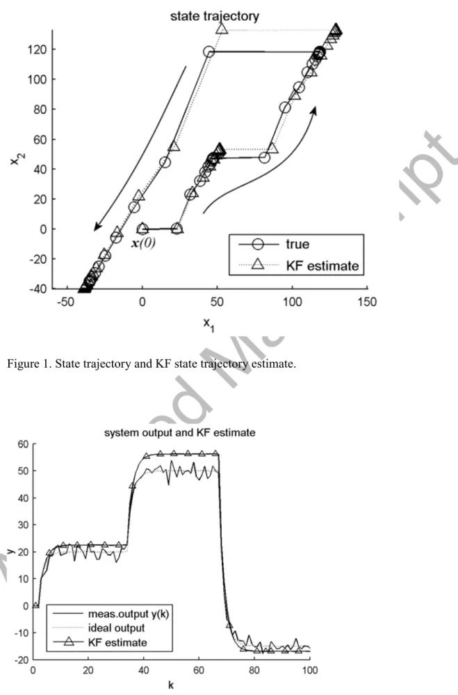
To illustrate this point, consider a set-point tracking problem in which the

system is controlled via a state-feedback control law according to

( ) = − ( ) + ( ) (9)

where is the vector of state-feedback gains, is a scaling gain calculated to ensure

that the overall steady-state closed-loop gain is unity, and is a prescribed reference

target for the system output. Let be chosen so that the closed-loop step-response has

zero overshoot (or unit damping), and a rise-time (0 to 90%) of < 5, for which a dominant closed-loop pole at 0.6 and a fast pole at 0.1 suffice, requiring a value of

= [0.1, −0.1625] and ≈ 0.852 (note that this control law is used by way of example to generate a realistic stabilising input ( ), but for the sole purpose of state-estimation, any other input could be prescribed instead).

(8)

Accepted

Manuscript

7

A simulation of the system is carried out for one hundred time-steps, with the

initial state being zero, and the target being set at 20, 50 and -15 for each one-third

of the simulation respectively. The disturbance and measurement noise sequences are

generated pseudo randomly according to the statistics given in (3). The state trajectory

of the system is then shown in Figure 1, and the output in Figure 2. Also shown in the

two figures are the KF estimates of the system state and output, for the same control

input, disturbance input, and output noise sequences, in which the model parameters

used by the filter have been overestimated by 5%. The KF initial estimate was taken

equal to the true initial state, and the initial error covariance as zero. One can clearly

observe that the KF estimates are biased due to the modelling error.

In practice, 100 percent accurate system modelling is utopian: at best, even in

the case of modelling via a first-principles approach, small modelling errors exist

because values of physical parameters (mass, geometry, resistivity, permittivity,

absorbance, etc.) can only be measured with a finite tolerance, not to mention that such

parameters are often sensitive to variable external factors, such as temperature, etc.

Tolerances, though, provide bounds to the models obtained.

If model parameters cannot be known with absolute precision, but bounds to

these are known, then the idea of describing system dynamics with interval values arises

naturally, ensuing in an interval model:

( + 1) = A ( ) + B ( ) + ( ) (10)

( ) = C ( ) + ( ) (11)

in which A, B and C are interval-valued matrices, that is, their elements are made up of bounded intervals, i.e. elements of the form

(9)

Accepted

Manuscript

8

, = , , , ; with , , , ∊ ℜ (12)

so that they can be written as

A = A ± ΔA = [A − ΔA, A + ΔA] (13)

B = B ± ΔB = [B − ΔB, B + ΔB] (14)

C = C ± ΔC = [C − ΔC, C + ΔC] (15)

where A, and C represent some nominal point-valued model.

In the late nineties a KF applied to interval system models was proposed by

Chen et al. (1997). Chen et al. leveraged the properties of an IA defined by Moore three

decades earlier (Moore, 1966). One of the basic tenets of Moore’s IA was that

calculations involving interval values must enclose every possible result that can be

obtained by operating on individual point-values contained within these. The resulting

interval thus guarantees bounds to the resulting set, though it may not equal it (a quality

known as the inclusion property). Using an extension of habitual statistical properties to

interval matrices and functions, Chet et al. constructed the IKF, whose equations ((16)

to (20)) mimic those of the ordinary KF, but provides state estimates in the form of

interval values. IKF equations: Prediction: ( | − 1) = A ( − 1| − 1) + B ( − 1) (16) P ( | − 1) = A P( − 1| − 1) A + Q (17) Kalman gain:

(10)

Accepted

Manuscript

9 K ( ) = P ( | − 1) C C P ( | − 1) C + R (18) Correction: ( | ) = ( | − 1) + K ( ) { ( ) − C ( | − 1)} (19) P ( | ) = { I − K ( ) C } P ( | − 1) (20)

Note that the state and error covariance estimates, as well as the Kalman gain, are now

interval-valued; however ( ) is point-valued as it is a measurement of the (true, not interval) output obtained via some sensor(s). The IKF, statistically optimal in the same

sense as the ordinary KF, provides interval state estimates which guarantee to contain

the KF estimates of every possible point-valued system contained in the interval model,

a consequence of the aforementioned inclusion property of IA. That is, it allows the

bounded uncertainty of the system model to be translated into bounds for the optimal

state estimates.

3. The wrapping effect

Assume that in the model (1) to (3) the elements of A, B, and C are known only to within 5% of the given values. Then the interval model (10) to (11), with

A = A ± 0.05 |A| = [A − 0.05 |A|, A + 0.05 |A|] (21)

B = B ± 0.05 |B| = [B − 0.05 |B|, A + 0.05 |B|] (22)

C = C ± 0.05 |C| = [C − 0.05 |C|, A + 0.05 |C|] (23) bounds the actual dynamics of the system, and the IKF estimates guarantee to contain

the optimal KF estimates of the system state (Chen et al., 1997). Based on the same

(11)

Accepted

Manuscript

10

inputs ( ) used in the previous simulation, and an initial state vector and error covariance given by

(0) = [−0.005, 0.005]_{[−0.005, 0.005] ; P} (0) = [0,0] [0,0]_{[0,0] [0,0]} (24)

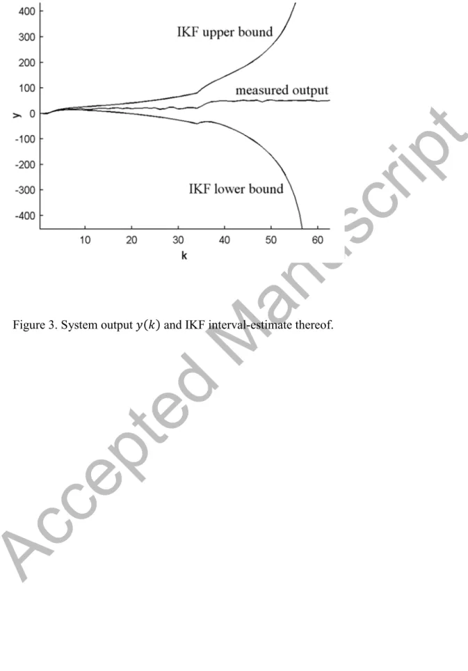
the upper and lower bounds of the IKF estimate of the output, C ( ), are shown in Figure 3, along with the actual output ( ). The IA was carried out in MATLAB using the IA package known as INTerval LABoratory (INTLAB), developed by Rump

(1999).

One thing is clearly apparent from observation of the figure: the widths of the

IKF interval-estimates expand exponentially, leading to bounds of the estimate that lose

any practical value. Moreover the figure only depicts the simulation of the IKF until

= 57: estimates of the bounds for = 60 and above were not possible as they surpassed the maximum and minimum IEEE 754 double precision floating point

representation (≈ 1.8 × 10 ).

One of the problems with IA is that direct computation yields over-conservative

results as a consequence of the inclusion property. This can be seen with a simple

example: consider an interval value = [− , ] , ∊ ℜ and ∊ ℜ, then

× ( − ) = × − × = [− , ] × − [− , ] × = [− × , × ] −

[− × , × ] = [−2 × , 2 × ] (25)

however, clearly the exact solution set is the single number zero. The overestimation

occurs because, after expansion of the brackets in the initial product, the arithmetic does

not remember that the interval variable in both terms represent the same variable. In

(12)

Accepted

Manuscript

11

the case of operations including interval vectors, the memory-less nature of IA has a

more severe effect.

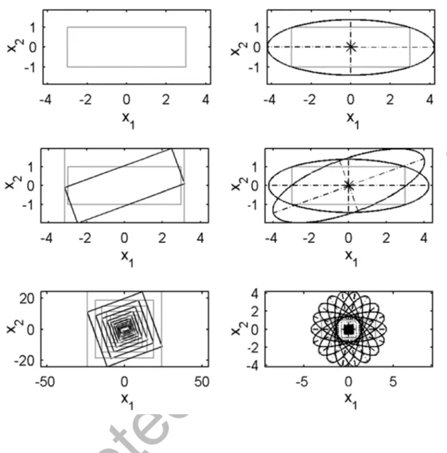
Consider an interval vector = [−3,3]_[−1,1] , which can be represented as a

rectangle (Figure 4), and the rotation matrix A = cos ( ) −sin( )_{sin ( )} _{cos ( ) , = 20 ×} . Then ≔ A represents the anticlockwise rotation of this rectangle by the angle (20°). Upon performing this operation using IA, the resultant enclosure is not the

rotated rectangle, but a rectangle with sides parallel to the coordinate axes that encloses

the former, which is consistent with the memory-less nature of IA described earlier,

since the correlation between the two dimensions given by the set of individually

rotated points is lost. The visual interpretation of this consequence has resulted in its

being known as the wrapping effect (Neumaier, 1993). The left column of Figure 4

depicts this process, first for a single rotation, and then ten successive applications of

the same, evidencing the ever-growing volume of the resulting rectangle; whereas the

actual transformed set is always the same size, given the volume preserving nature of A, which is an orthogonal matrix. This process clearly shows that direct application of IA

can be overly-conservative. However, as shown in the right column of Figure 4, if the

initial rectangle is first enclosed by an ellipse, then each successive rotation of the

ellipse does not need to be “wrapped” before a successive rotation is applied, since

ellipses are preserved under rotations, and in general, ellipsoids under affine

transformations. Indeed, let be the set of points of the ellipsoid E( , L, )

∶= { + L ∶ ∊ ℜ , ‖ ‖ ≤ }, ∊ ℜ , L ∊ ℜ × _{, ∊ ℜ} _{, then, the set of points}

transformed by the affinity ≔ A + b, A ∊ ℜ × , , ∊ ℜ , is given by the ellipsoid

E( ̅, L, ), with ̅ = A + b and L = A L.

(13)

Accepted

Manuscript

12

4. A hybrid ellipsoidal-rectangular IA enclosure algorithm for recursive interval affine transformations

In the previous section, the advantage of using ellipsoidal arithmetic over (rectangular)

IA for recursive affine transformations of sets in order to avoid the wrapping effect was

made apparent. However, whilst ellipsoids are conserved under affine transformations,

they are not so under interval transformations. In the case of an interval affine

transformation, ≔ A + b, a practicable ellipsoidal enclosure to the set of transformed points must be sought. Neumaier (1993) has developed a method that

guarantees such an enclosure with a certain degree of optimality. The main results of

this method are summarised next.

Let be the set of points of the ellipsoid E( , L, ) ∶= { + L ∶ ∊ ℜ , ‖ ‖ ≤

}, ∊ ℜ , L ∊ ℜ × _{, ∊ ℜ} _{, and} _{≔ A + b, A ∊ A , b ∊ b}_{an interval affine}

transformation of ∊ ℜ , with A and b an × and × 1 interval-valued matrix and vector respectively. Neumaier shows that for any ̅ ∊ ℜ , L ∊ ℜ × , if ̃ =

‖L (A + b − )‖ + ‖L A L‖ , then A + b ∊ E( ̅, L, ̃) ∀ A ∊ A , b ∊ b , ∊ . This allows one to find an (ellipsoidal) enclosure for the interval affine transformed

points of , but such enclosure may by no means be “tight”.

However, let ̅ = (A + b ), = |A + b − |, B = (A L), and

′ = (A L − B), where is the Frobenius norm. Then, for any non-singular L and any non-singular diagonal matrix D, it can be verified that ̃ ≤ ‖L B‖ + ‖L D‖ , where

= ‖D ‖ + ‖D ′‖ . In particular, for an L that satisfies BB + DD = LL , then it is shown that ̅ = ‖L B‖ + ‖L D‖ ≤ 2 and that

| L| ≤ L L B + L D for any non-singular L, that is, that this choice of L provides an ellipsoid enclosure that is optimal to within a factor of 2 of the radius (note that L L B + L D is an upper bound to the volume of the

(14)

Accepted

Manuscript

13

ellipsoid for the arbitrarily chosen L). However, it is also noted that the optimality of the radius chosen is subject to that of the bound ̃ ≤ ‖L B‖ + ‖L D‖ .

The choice of L and D still remains non-uniquely determined, and for reasons of computational stability, L is obtained as a Cholesky factor of BB + DD and

D = { + }.

In summary, this procedure provides an ellipsoidal enclosure for the image-set

of the points belonging to an initial ellipsoid by an interval affine transformation. In

practice, to use this method for propagating the state vector of a dynamic system given

an initial interval vector, which is representable by an n dimensional hyper rectangle, or

box, an ellipsoidal enclosure to this initial state is first calculated. Although the ellipsoid

circumscribing a given box is not unique, one option is to choose the minimal volume

circumscribing ellipsoid, and is the method adopted in the subsequent examples.

Consider the simulation of the interval system (10) and (11), with A, B , & C given by (21) to (23), where the nominal values of the interval matrices are the ones

specified in (3), using the same inputs ( ) used in the previous simulation, and with an initial interval-valued state vector given by

(0) = [−0.005, 0.005]_{[−0.005, 0.005]} (26)

Figure 5(a) depicts the propagation of the state intervals using (rectangular) IA,

whereas Figure 5(b) shows the same calculations but using ellipsoidal arithmetic with

Neumaier’s enclosures. Clearly the elliptical enclosures are far tighter than the

corresponding rectangular ones. Note that the interval affine transformation of the

interval state vector at each time-step is given by (10), in which A represents a linear interval transformation (i.e., set of linear transformations), and b ( ) ≝ B ( ) +

( ) an interval translation vector (i.e. set of translations). The eigenvalues of the

(15)

Accepted

Manuscript

14

nominal linear transformation, A, are the complex conjugate pair 0.4 ± 0.25 , so the system is somewhat underdamped.

Now consider the simulation of an interval system with nominal overdamped

dynamics given by

A = 0.6 −0.05

1 0 , B = 10 , C = [0 1] (27)

and interval matrices centred around these nominal ones with interval widths of 5% on

either side, as stated in (21) to (23). As before, simulation is carried out for one-hundred

time-steps, with a reference target being set at 20, 50 and -15 for each one-third of

the simulation respectively, and a state-feedback control law as in (9) with =

[−0.1, 0.01] and = 0.8 calculated to have the same closed-loop poles as before (0.6 and 0.1) (note that for generating the control input, the true state of the system is used,

as the main concern here is not the control law generated but the calculation of the

interval state trajectory). The resulting state propagation using (rectangular) IA and

ellipsoidal arithmetic are shown in Figures 6(a) and 6(b) respectively, with the initial

state being described by (26). In this case, IA provides tighter bounds to the state-vector

sets than does ellipsoidal arithmetic. It is interesting to note that in this case, the

nominal poles of the system are at 0.5 and 0.1.

The tightness of the ellipsoidal enclosures computed according to Neumaier’s

algorithm depends on the nature of the linear interval transformation matrix A. If the eigenvalues are predominantly complex conjugate (corresponding to underdamped

systems), then the transformation has a greater rotation component, and Neumaier’s

enclosures work well. On the other hand, for real eigenvalues (corresponding to

overdamped systems), the transformation has a larger shear component, and the

(16)

Accepted

Manuscript

15

ellipsoid enclosures become very elongated in the direction of largest stretching. Thus it

becomes a necessity to develop a method that can be of use in either situation.

In order to provide enclosures that are tight for both under and overdamped

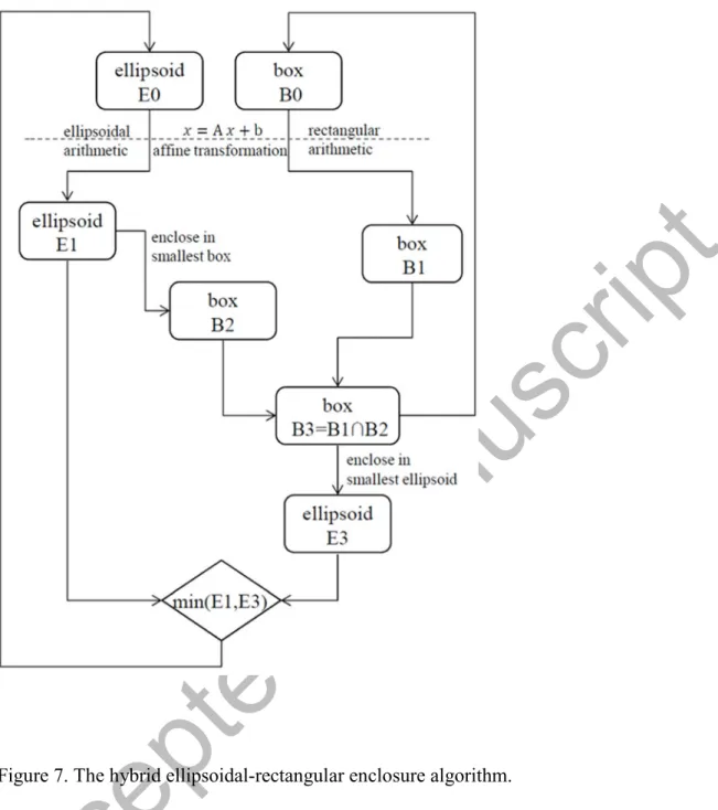
systems, the following algorithm is proposed for recursive affine transformations. Given

an initial interval vector, which is an n-dimensional box, B0, obtain the smallest ellipsoid containing it, E0. The word “smallest” is used here vaguely, but one option (and the one implemented here) is to choose the ellipsoid with the smallest volume that

contains the box, that is, an ellipsoid with the same eccentricity as the box. Then

proceed to apply the interval affine transformation to both enclosures, B0 via

(rectangular) IA and E0 via ellipsoidal arithmetic, resulting in B1 and E1, respectively. Note that the tightest set containing the transformed points at this stage will be given by

the intersection of B1 and E1, which however is in general neither a box nor an

ellipsoid. Thus, obtain the tightest box B2 that contains E1, which, intersected with B1 results in B3. The box B3 is now the smallest box-enclosure that contains the

transformed set, and is used as the starting box for the next interval transformation. On

the other hand, obtain E3 as the smallest ellipsoid containing B3. Then select the smaller of E1 and E3 as the starting ellipsoid to be transformed by the next interval affine transformation. Again, smaller in this case could be in terms of volume, sum of

semi-axes, etc. The algorithm is summarised in Figure 7.

5. The IKF equations as affine transformations

The ellipsoidal arithmetic approach is possible because ellipsoids are invariant under

affine transformations. In order to be able to apply ellipsoidal arithmetic to the IKF

equations, these must first be expressed as recursive affine transformations. The IKF

equations were given in (16) to (20) and can be divided into three sets: propagation of

(17)

Accepted

Manuscript

16

the state-vector, propagation of the error covariance, and calculation of the Kalman

gain.

With respect to propagation of the state vector, (16) and (19) must be applied in

turn. The prediction equation (16) is already in the form of an interval affine

transformation, whereas (19) can be written as

( | ) = { I − K ( ) C } ( | − 1) + K ( ) ( ) (28)

which, if K ( ) has already been obtained, is also clearly an interval affine transformation.

For the error covariance estimates, consider the prediction equation (17) written

using indicial notation:

, ( | − 1) = , , , ( − 1| − 1) + , ; , , , = 1, … , (29)

In order to represent the state estimate error and disturbance covariance matrices as

vectors, consider ( | − 1), ( − 1| − 1), and ∊ ℜ defined as:

( ) ( | − 1) ≝ , ( | − 1) , , = 1, … , (30)

19 ℎ _, ≝ { I − K ( ) C } , if , ∊ { , + 2, … , + ( − 1)} 0 otherwise , = 1, … , ; , = 1, … , (47)

Then, (42) can be written as

( | ) = ℎ , ( | − 1) ; , = 1, … , (48)

which is clearly in the form of an affine transformation.

For example, for = 2, the error covariance prediction equation is

, ( | − 1) , ( | − 1) , ( | − 1) , ( | − 1) = , , , , , ( − 1| − 1) , ( − 1| − 1) , ( − 1| − 1) , ( − 1| − 1) , , , , + q _, q _, q , q , (49)

which can be expressed as

( | − 1) ( | − 1) ( | − 1) ( | − 1) = , , , , , , , , , , , , , , , , , , , , , , , , , , , , , , , , ( − 1| − 1) ( − 1| − 1) ( − 1| − 1) ( − 1| − 1) + (50) where

(21)

Accepted

Manuscript

20 ( | − 1) ( | − 1) ( | − 1) ( | − 1) ≝ , ( | − 1) , ( | − 1) , ( | − 1) , ( | − 1) , ( − 1| − 1) ( − 1| − 1) ( − 1| − 1) ( − 1| − 1) ≝ , ( − | − 1) , ( − | − 1) , ( − | − 1) , ( − | − 1) & ≝ q _, q , q _, q _, (51)

Similarly, the error covariance correction equation is

, ( | ) , ( | ) , ( | ) , ( | ) = ℎ , ℎ , ℎ _, ℎ _, , ( | − 1) , ( | − 1) , ( | − 1) , ( | − 1) (52) which is equivalent to ( | ) ( | ) ( | ) ( | ) = ℎ _, 0 0 ℎ _, ℎ _, 0 0 ℎ _, ℎ _, 0 0 ℎ _, ℎ _, 0 0 ℎ _, ( | − 1) ( | − 1) ( | − 1) ( | − 1) (53) if ( | ) ( | ) ( | ) ( | ) ≝ , ( | ) , ( | ) , ( | ) , ( | ) (54)

Finally, the Kalman gain is updated as a rectangular enclosure at each step

according to (18) directly using IA.

(22)

Accepted

Manuscript

21

6. Interval Kalman filtering using the hybrid ellipsoidal-rectangular enclosure algorithm

Consider again the simulation of the two interval systems of the preceding section,

namely, the systems described by (10) and (11), with A, B , & C given by (21) to (23), and nominal values of the interval matrices given, in the first case, by (3) (underdamped

nominal dynamics), and in the second, by (27) (overdamped nominal dynamics). For

each case, using the same inputs ( ) used in the preceding section, and the same disturbance and noise processes described earlier, the state-trajectory and output of the

nominal system are simulated from an initial state situated at the origin of the

state-space. Also, based on the initial estimates given in (24), the IKF equations are in turn

simulated using purely IA based computations, via the ellipsoidal arithmetic recursions

described in the preceding section, and lastly using the hybrid ellipsoidal-rectangular

enclosure algorithm. The resulting state enclosures at each time step are depicted in

Figures 8 to 11.

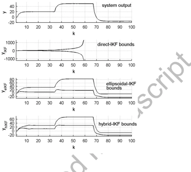
As seen from the figures, in the case of the underdamped system with complex

conjugate poles, the rectangular enclosures obtained via IA overestimate the actual state

sets to such an extent that simulation cannot continue after a certain point, whereas the

ellipsoidal arithmetic IKF provides much tighter bounds. The hybrid enclosure IKF in

this case offers bounds similar to those of the ellipsoidal arithmetic IKF. In the case of

the overdamped system with real poles, however, it is the rectangular IA IKF enclosures

that provide the tighter bounds to the sets of state vectors, and so the hybrid enclosure

IKF relies mostly on these.

7. Conclusions

For systems with bounded modelling uncertainty, the IKF provides guaranteed

bounds to the optimal estimate of the state vector. Even if the exact values of the states

(23)

Accepted

Manuscript

22

are not known, guaranteed bounds to these can be useful, for example, to ensure that

they remain within some desirable or permissible operating region. However,

implementation of the IKF via IA can result in over conservative bounds which are not

representative of the actual set of possible optimal states, and in some cases can even

grow indefinitely. It thus becomes necessary to develop alternative methods by which to

compute the IKF estimates which yield stable and tighter bounds.

The case studies presented in this paper show that implementation of the IKF

equations by means of the hybrid enclosure algorithm provides stable and tighter

bounds for a wider range of system dynamic characteristics than does the direct

application of IA which generates rectangular enclosures. The hybrid enclosure

approach is based on using ellipsoidal arithmetic as well as IA to propagate both an

ellipsoidal and rectangular enclosure of the state vector at each time step, respectively,

and subsequently fusing these prior to the next iteration. These fusions only require the

intersecting of boxes and circumscribing these by ellipsoids, and are computationally

inexpensive.

Although it was shown that for certain types of systems the rectangular IA

enclosures consistently provide tighter bounds than the ellipsoidal arithmetic ellipsoids,

and that for another class of systems the opposite occurs, the advantage of using the

hybrid enclosure approach over one or other set arithmetic is that for borderline cases

the more effective type of enclosure may alternate from iteration to iteration. Moreover,

in practice the dynamics of a system can be prone to large scale variations. Control

strategies for such systems are often based on multiple model representations of the

same. Thus, even though the large scale dynamical changes in the nominal model of the

system may be known, it is necessary to use an IKF implementation that is effective for

a broad spectrum of possible dynamic characteristics.

(24)

Accepted

Manuscript

23

Furthermore, it should also be noted that if the closed-loop dynamics of the

system are specified, such as in the examples shown here, then the IKF may be defined

directly upon the resulting closed loop interval model obtained from applying the

feedback control law to the uncertain open-loop model. The IKF implementation must

therefore be robust to the choice of desired closed-loop specifications, or changes to

these specifications over time.

For the aforementioned reasons, the use of the hybrid enclosure implementation

is clearly advantageous. Its mathematical development has been presented for generic

linear state space models of any order, and its application will enable the practical and

efficient use of the IKF as a guaranteed state estimator for all kinds of systems with

bounded parametric uncertainty that respond to the linear model. Suggested future

research includes further sharpening of the interval bounds by incorporating the

calculation of an enclosure to the Kalman gain into the recursive ellipsoidal arithmetic

scheme, or finding an alternative arithmetic that can implement all of the IKF equations.

Another useful development would be the extension of the method to the nonlinear case

(interval extended KF).

Nomenclature

KF Kalman filter

IKF Interval Kalman filter

INTLAB Interval laboratory

IA Interval arithmetic

A(A ) real (interval) valued state transition matrix / linear transformation matrix

(25)

Accepted

Manuscript

24

B(B ) real (interval) valued input matrix

C(C ) real (interval) valued output matrix

E( , L, ) set of points { + L ∶ ∊ ℜ , ‖ ‖ ≤ }, ∊ ℜ , L ∊ ℜ × , ∊ ℜ

K(K ) real (interval) valued Kalman gain state feedback gain vector

scaling gain

I identity matrix

Iℜ set of nonempty, closed and bounded real intervals normal distribution

P(P ) real (interval) valued error covariance matrix

Q input disturbance covariance matrix

R output noise covariance matrix

ℜ(ℜ ) set of real (positive real) numbers

( ) interval valued (augmented) state transition matrix

b(b ) linear (linear interval) translation vector

ℎ interval valued error covariance transition matrix iteration number

, (i,j)th element of

( ) interval valued error covariance matrix (vector)

( ) interval valued input disturbance covariance matrix (vector) input or control vector

real state vector

( ) real (interval) state vector estimate output vector

reference output

(26)

Accepted

Manuscript

25

|. | element wise absolute value

‖. ‖ Euclidean norm

∶= assignment operator

Δ increment angular value

output noise vector / Frobenius norm

disturbance input vector

References

Ahn, H., Kim, Y., & Chen,Y. (2012). An interval Kalman filtering with minimal conservatism. Applied Mathematics and Computation, 218(18), 9563-9570. Bertsekas, D., & Rhodes, I. (1971). Recursive state estimation for a set-membership

description of uncertainty. IEEE Transactions on Automatic Control, 16(2), 117-128.

Chen, G., Wang, J., & Shieh, L. S. (1997). Interval Kalman Filtering.IEEE Transactions on Aerospace and Electronic Systems, 33(1), 250–258.

Gao, H., & Chen, T. (2007). H-Infinity estimation for uncertain systems with limited communication capacity. IEEE Trans. on Automatic Control, 5(11), 2070-2084. He, X. F., and Vik, B. (1999). Use of Extended Interval Kalman Filter on Integrated

GPS/INS System. Proceedings of the 12th International Technical Meeting of the Satellite Division of The Institute of Navigation, (pp. 1907-1914). Nashville, TN.

Jain, B. N. (1975). Guaranteed error estimation in uncertain systems. IEEE Transactions on Automatic Control, 20(2), 230-232.

Jaulin, L. (2009). Robust set membership state estimation. Application to Underwater Robotics. Automatica, 45(1), 202-206.

Julier, S., & Uhlmann, J. (1997). A new extension of the Kalman filter to nonlinear systems. Proc. of AeroSense: The 11th Int. Symp. on Aerospace/Defense Sensing, Simulations and Controls (pp. 182-193). Orlando, FL, USA.

Kalman, R. E. (1960). A New Approach to Linear Filtering and Prediction Problems.

Transactions of the ASME, Journal of Basic Engineering, 82, 35-45.

(27)

Accepted

Manuscript

26

Moore, R. E. (1966). Interval Analysis. Prentice-Hall, Englewood, NJ.

Motwani, A., Sharma, S. K., Sutton, R., & Culverhouse, P. (2013). Interval Kalman Filtering in Navigation System Design for an Uninhabited Surface Vehicle.

Journal of Navigation, 66, 639-652.

Neumaier, A. (1993).The wrapping effect, ellipsoid arithmetic, stability and confidence regions. Computing Supplementum, 9, 175-190.

Petersen, I. R., & McFarlane, D. C. (1996). Optimal guaranteed cost filtering for uncertain discrete-time linear systems. Int. J. Robust Nonlinear Control, 6, 267– 280.

Rump, S. (1999). INTLAB - INTerval LABoratory. Kluwer Academic Publishers. Savkin, A. V., & Petersen, I. R. (1998). Robust state estimation and model validation

for discrete-time uncertain systems with a deterministic description of noise and uncertainty. Automatica, 34(2), 271-274.

Sayed, A. H. (2001). A framework for state-space estimation with uncertain models.

IEEE Trans Autom Control, 47, 998–1013.

Siouris, G., Chen, G. and Wang, J. (1997). Tracking an Incoming Ballistic Missile using an Extended Interval Kalman filter. IEEE Transactions on Aerospace and

Electronic Systems, 33(1), 232–240.

Smith, G., A., Schmidt, S. F., & McGee, L. A. (1961). Application of statistical filter theory to the optimal estimation of position and velocity on board a circumlunar vehicle (Technical Report R-35). Moffett Federal Airfield, CA.

Tiano, A., Zirilli, A., Cuneo, M. and Pagnan, S. (2005). Multisensor Data Fusion Applied to Marine Integrated Navigation Systems. Proceedings of the IMechE Part M: Journal of Engineering for the Maritime Environment, 219(3), 121-130. Tiano, A., Zirilli, A., & Pizzocchero, F. (2001). Application of interval and fuzzy

techniques to integrated navigation systems. Joint 9th IFSA World Congress and 20th NAFIPS International Conferenceproceedings, 1 (pp.13-18). Vancouver, British Columbia, Canada.

Manuscript

29

Figure 3. System output ( ) and IKF interval-estimate thereof.

(31)

45

Figure 11. Output of the nominal overdamped system, and IKF bounds to the estimates of the output of the corresponding interval system using IA, ellipsoidal arithmetic, and hybrid enclosures respectively.