University of Pennsylvania
ScholarlyCommons
Finance Papers
Wharton Faculty Research
1-23-2017
Volatility and Venture Capital
Ryan Heath Peters
University of Pennsylvania
Follow this and additional works at:
http://repository.upenn.edu/fnce_papers
Part of the
Finance and Financial Management Commons
This paper is posted at ScholarlyCommons.http://repository.upenn.edu/fnce_papers/31 For more information, please [email protected].
Recommended Citation
Volatility and Venture Capital
Abstract
The performance of venture capital (VC) investments load positively on shocks to aggregate return volatility. I document this novel source of risk at the asset-class, fund, and portfolio-company levels. The positive relation between VC performance and volatility is driven by the option-like structure of VC investments, especially by VCs’ contractual option to reinvest. At the asset-class level, shocks to aggregate volatility explain a substantial fraction of VC returns. At the fund level, consistent with the reinvestment channel, this exposure is
concentrated in years two through four of fund life and in early-stage VC funds, which have more embedded reinvestment options. For VC-backed portfolio companies, volatility shocks correlate with faster and more frequent reinvestment. The level of volatility at the time of investment has no relation with future
performance, consistent with competitive markets. Overall, my results imply that the option-like features of VC investments are first-order determinants of risk in VC.
Keywords
venture capital, real options, idiosyncratic volatility Disciplines
Volatility and Venture Capital
Ryan H. Peters* January 23, 2017
JOB MARKET PAPER LINK TO LATEST VERSION
Abstract:
The performance of venture capital (VC) investments load positively on shocks to aggregate return volatility. I document this novel source of risk at the asset-class, fund, and portfolio-company levels. The positive relation between VC performance and volatility is driven by the option-like structure of VC investments, especially by VCs’ contractual option to reinvest. At the asset-class level, shocks to aggregate volatility explain a substantial fraction of VC returns. At the fund level, consistent with the reinvestment channel, this exposure is concentrated in years two through four of fund life and in early-stage VC funds, which have more embedded reinvestment options. For VC-backed portfolio companies, volatility shocks correlate with faster and more frequent reinvestment. The level of volatility at the time of investment has no relation with future performance, consistent with competitive markets. Overall, my results imply that the option-like features of VC investments are first-order determinants of risk in VC.
JEL codes: G11, G24
Keywords: Venture Capital, Real Options, Idiosyncratic Volatility
* The Wharton School, University of Pennsylvania. Email: [email protected].
I thank Lucian Taylor, Nikolai Roussanov and Jessica Wachter, my dissertation committee, for their con-tinual support and guidance. I also thank Garth Baughman, Jules van Binsbergen, Jessica Jeffers, Olivia S. Mitchell, Christian Opp, Rob Stambaugh and Pavel Zryumov for helpful discussions as well as seminar participants at the Federal Reserve Board, The University of Pennsylvania (Wharton) and University of Gothenburg (CFF). I thank the Private Equity Research Consortium, the Institute for Private Capital, Burgiss and Dow Jones VentureSource for research support and access to data and gratefully acknowledge financial support from the Rodney L. White Center for Financial Research, the Jacobs Levy Equity Man-agement Center for Quantitative Financial Research and the Mack Institute for Innovation ManMan-agement. The latest version of this paper can be found at http://goo.gl/xMZ74C
1
Introduction
This paper identifies a novel source of risk that helps to explain the observed time-series patterns in venture capital (VC) investment performance: exposure to shocks to the level of aggregate idiosyncratic return volatility. While idiosyncratic shocks are by definition mean-zero return shocks, the level of idiosyncratic volatility drives VC returns through the value of the real options embedded in VC contracts. When volatility increases, these real options become more valuable, improving VCs’ performance. This paper examines the extent to which this exposure can explain observed patterns in VC investment performance and dynamics and identifies the primary channel driving this empirical relationship.
Two common contractual channels of VC investments generate option-like characteristics. The first is the liquidation preference given to investors, which entitles them to recuperate at least their initial investment before other investors participate in proceeds from any potential firm exit. These liquidation preferences imply a nonlinear payoff structure similar to those in equity options. The second channel is the (real) reinvestment option embedded in the contracts that VCs write with their portfolio companies, namely a right of first refusal for participation in future financing rounds.1
There are a number of other reasons why idiosyncratic volatility might be especially important to the VC sector. First, VC returns are known to be highly skewed. Metrick and Yasuda (2011), among others, show that a very large share of the total returns in VC come from a small fraction of their investments. Additionally, the compensation structure of VC general partners (GPs) themselves (eg. two and twenty) encourages the construction of portfolios that have a high total return variance, and thus a high idiosyncratic volatility. Moreover, VCs traditionally invest in the types of firms (small, high-tech) whose idiosyncratic volatility is high and loads heavily on aggregate changes in idiosyncratic volatility. While each of these characteristics of VC investments suggest that idiosyncratic volatility may be particularly large, none of them suggest that changes in the level of idiosyncratic volatility should drive returns.
1Bergemann and Hege (1998, 2005) demonstrate that these contractual features emerge from the contracting
I investigate the empirical relation between VC investments and innovations in aggregate id-iosyncratic volatility at three levels of aggregation. First, at the asset class level, I measure the exposure of VC benchmark portfolios to changes is aggregate idiosyncratic volatility. Second, I use detailed data on investor cash flows to investigate the time heterogeneous exposure of individual VC funds to innovations in asset volatility during those funds’ lives. The third level of aggregation is at the level of individual investments by VCs into their portfolio companies, where I investigate the extent to which idiosyncratic volatility is related to the process by which VCs invest.
Rather than directly constructing a measure of VC portfolio company idiosyncratic volatility, I use a measure of the idiosyncratic volatility of publicly traded equities from Herskovic, Kelly, Lustig, and Van Nieuwerburgh (2016) as a proxy for the idiosyncratic volatility of VC-backed firms. I use a public market proxy for two reasons. First, return data on publicly traded equity is of better quality and available at a much higher frequency, allowing for high-frequency estimates of idiosyncratic volatility shocks. The second reason is that using a measure from public markets minimizes potential endogeneity concerns.2
There are a number of reasons to believe that the idiosyncratic volatility of VC-backed firms is strongly related to that from public markets. First, Herskovic et. al. (2016) show that publicly traded firms’ idiosyncratic volatility obeys a strong factor structure, i.e. that the level of idiosyn-cratic volatility is highly correlated across firm sizes and industries. Additionally, they find that the idiosyncratic volatility of small firms along with high-tech and health-related firms, the types of firms typically financed by VC funds, are more sensitive to this common factor. Finally, I validate the measure by comparing low frequency estimates of VC-backed firm idiosyncratic volatility to similarly timed low frequency measures from publicly traded firms and show that these two series move together strongly.
I begin the main empirical analysis by establishing that commonly used VC benchmark return indexes load positively on idiosyncratic volatility shocks. In particular, factor regressions for these VC indexes have significantly higher R2 when including idiosyncratic volatility shocks. In other
2
One potential source of endogeneity is the fact that the amount of experimentation done by VCs, and therefore the idiosyncratic volatility of VC-backed firms, may be endogenously determined by the amount of capital available to VCs for investment as argued by Nanda and Rhodes-Kropf (2013, 2016).
words, idiosyncratic volatility shocks explain a large fraction of the variance of VC industry returns after accounting for the fraction explained by market returns. I incorporate lagged regressors in these factor regressions to account for asynchronous prices of privately traded firms as discussed in Dimson (1979), and find that a one quarterly standard deviation innovation to the level of idiosyncratic volatility corresponds to an approximately 8% return in the VC index. This effect is even larger for a benchmark index of early-focused VC performance.
If the price of volatility risk is non-zero, this exposure has implications for the risk-adjusted performance of VC investments. There is a large body of theoretical and empirical work3 that suggests the price of volatility exposure is negative, i.e. that investors are willing to pay for exposure to this risk. In this case, the positive exposure to this risk documented in this paper implies that the risk-adjusted performance of VC investments is higher than previously believed. I test this hypothesis by measuring the exposure of VC benchmark return indexes to a tradeable portfolio of equity options constructed to proxy for idiosyncratic volatility risk, and find that accounting for this tradeable factor increases the risk-adjusted performance of venture capital investments by as much as 6% per year.
Next, in order to relate these shocks to investor cash flows directly and investigate the potential channels driving this empirical relationship, I examine the exposure of individual venture capital funds to changes in aggregate idiosyncratic volatility. I use the realized cash flows between investors and the VC funds in which they invest from Burgiss. This data is sourced from a diverse array of limited partners (fund investors) for whom Burgiss provides investment decision support tools and includes a complete transaction and valuation history between the LPs and fund investments.
The fund performance measure I use is the public market equivalent (PME) of Kaplan and Schoar (2005), which accounts for the opportunity cost of capital.4 I find a significant relation between fund PME and idiosyncratic volatility shocks over the life of the fund and, in particular, those shocks that occur in years two and three of the fund’s life. This finding is consistent with the reinvestment option channel, since by year two most initial investments will have been made, and
3
See Mankiw (1986), Constantinides and Duffie (1996) and Herskovic, Kelly, Lustig and Van Nieuwerburgh (2016).
4
Specifically, the PME provides a valid economic performance measure when the LP has log-utility preferences and the return on the LP’s total wealth equals the market portfolio (Sorensen and Jagannathan, 2015). I also examine the effect of loosening these restrictions, as in, for example, Korteweg and Nagel (2016).
by year 5 VC fund managers are looking to exit their positions. I also estimate the strength of this exposure in funds with different investment focus. The relation is much stronger for those funds which focus on early-stage investments, where reinvestment options inherently plays a larger role, than in late-stage investment focused funds. In a placebo analysis, I show that buyout funds, which buy target companies whole and therefore have no reinvestment options, exhibit no exposure to volatility shocks. This suggests that exposure to aggregate idiosyncratic volatility is not a feature of private equity investments more broadly.
At the level of VC investments into portfolio companies, I use cash-on-cash multiples and an-nualized returns as the measures of performance, controlling throughout for public equity prices (Tobin’s q) and returns. I find that investments made when idiosyncratic volatility is high do not have higher average returns than those made at other times, consistent with the level of id-iosyncratic volatility being priced into individual VC financing deals, as would be expected. What does drive investment-level returns are shocks to the level of idiosyncratic volatility after the initial investment. This relationship is again much stronger for early investment rounds, consistent with the reinvestment channel. I also find that reinvestments happen faster and are more likely in times of rising idiosyncratic volatility, suggesting that these innovations have a direct relationship with the amount of capital available to entrepreneurs.
Taken together, these results imply a strong effect of aggregate idiosyncratic volatility shocks on investment returns and dynamics in VC investments. This effect can help us to understand the time-series of VC investment dynamics and rationalize the large differences in risk-adjusted returns observed at different times in the existing literature. Moreover, the results imply that the real options embedded in VC investments are a first-order determinant of risk in VC.
This paper relates to the literature surrounding the impact of contractual and informational frictions on VC investments. In particular, Ewens, Jones and Rhodes-Kropf (2013) demonstrate how the principal-agent problem between VCs and their investors cause private equity fund returns to depend on diversifiable risk in the cross section of funds. This effect is distinct from the time-series relationship investigated in this paper. In addition, their cross-sectional results hold for both VC and buyout funds, while the results in this paper hold only for VC funds. This result makes
sense because the reinvestment options which are the focus of this paper are only present in VC investments. Cornelli and Yosha (2003) show that staged financing helps to mitigate the problem of manipulation for purposes of window-dressing. Fluck, Garrison, and Myers (2007) highlight the role of staged financing as a real option and show that it alleviates the effort provision problem.
There is also a substantial literature on the risk and return characteristics of VC investments: Cochrane (2005), Kaplan and Schoar (2005), Hall and Woodward (2007), Korteweg and Sorensen (2010), and Korteweg and Nagel (2016). A large literature on the implications of idiosyncratic risk for entrepreneurs and managers is summarized by Heaton and Lucas (2004) and Hall and Woodward (2010). This paper differs from the previous literature by explicitly accounting for the role of idiosyncratic volatility in return dynamics.
This paper also relates to a large empirical literature on the role of idiosyncratic return volatility. Campbell, Lettau, Malkiel, and Xu (2001) examine secular variation in average idiosyncratic return volatility. Wei and Zhang (2006) study aggregate time-series variation in fundamental volatility. Engle and Figlewski (2015) document a common factor in option-implied volatilities. Jurado, Ludvigson, and Ng (2015) study measures of uncertainty from aggregate and firm-level data and relates them to macroeconomic activity. Ang, Hodrick, Xing, and Zhang (2006) show that stocks with high idiosyncratic volatility earn abnormally low average returns. This paper adds to this literature by identifying VC as a sector that is particularly exposed to idiosyncratic volatility risk. The rest of the paper proceeds as follows: Section 2 presents two potential channels of volatility exposure. Section 3 introduces the VC data and the idiosyncratic volatility measure and compares public and private market idiosyncratic volatility. Section 4.1 presents empirical results using VC-industry return indexes. Section 4.2 presents empirical results using investor cash flows while section 4.3 presents empirical results using investment-level data. Section 5 concludes.
2
Sources of Volatility Exposure
This section briefly describes two potential channels through with VC investments may be exposed to shocks to the volatility of their underlying assets. The first channel is through the liquidation preference given to investors through the convertible preferred equity structure common to VC
investments. This contractual feature of VC contracts induces both concavity and convexity in the VC payoff, which can lead to volatility exposure. The second channel is the (real) reinvestment option embedded in the contracts that VCs write with their portfolio companies. These contracts frequently include a contractual right of participation in future investment rounds which can again lead to a volatility exposure of the vale of the security. Both liquidation preferences and staged investment emerge from the contracting environment with information asymmetry (Bergemann and Hege (1998, 2005)), an inherent friction in the financing of small, private firms. A third potential explanation of the idiosyncratic volatility exposure of VC is that the underlying assets, the portfolio companies themselves, are positively exposed to volatility shocks.
2.1 Liquidation Preferences
Kaplan and Stromberg (2003) report that of 213 rounds of financing, all but one contained some form of liquidation preference. A standard specification of the liquidation preference takes the following form in the National Venture Capital Association’s (NVCA) 2013 model term sheet:
In the event of any liquidation, dissolution or winding up of the Company, the proceeds shall be paid as follows: First pay [x] times the Original Purchase Price ... on each share of Series A Preferred. Thereafter, the Series A Preferred participates with the Common Stock pro rata on an as-converted basis.
Typically, the liquidation preference amounted to the lesser of the liquidation value of the firm and the VC’s original investment (x= 1) and may include an unpaid cumulative dividend (45% of cases) that raises this amount over time.
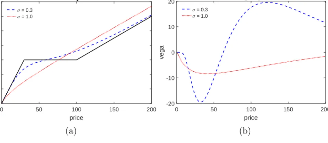
Panel (a) of Figure 1 shows a payoff diagram for a typical convertible preferred equity stake.5 The dashed line represents the payoff to a participating convertible preferred equity investor holding a certain ownership share in the firm (in this case 30%). The dashed (blue) line represents the value before the final payoff is realized, as calculated using the Black-Scholes model assuming an annualized volatility of 30% while the dotted (red) line assumes an annualized volatility of 100%,
5
A number of theoretical papers rationalize this form of equity participation by investors, eg. Cornelli and Yosha (2003), DeMarzo and Sannikov (2006), DeMarzo and Fishman (2007), and Biais, Mariotti, Plantin and Rochet (2007)
which is close to the average idiosyncratic volatility of VC-backed firms (see Section 3.5).6 The distance between the dotted and solid lines represents the extrinsic value of the option and is directly related to the volatility of the underlying asset. The volatility exposure, orvega, of a long call option is positive and easily calculated as:
∂C ∂σ =S r T 2πe −(log(S/X)+(r+σ2/2)T)2/(2σ2T) , (1)
where T is the time until option expiration, r is the interest rate, X is the strike price, σ is the underlying volatility and S is the value of the firm. Panel (b) shows the vega of the convertible preferred equity position.
Figure 1 shows that when the volatility is relatively low the direction of the volatility exposure is ambiguous. However, when the volatility is high enough, and in particular is the level observed for VC-backed firms, the negative volatility exposure of the concave part of the payoff is potentially larger than that from the convex part. This implies that this particular contractual feature of VC investments is unlikely to drive the positive volatility exposure of VC returns.
2.2 A Simple Model of Idiosyncratic Volatility and Reinvestment
An alternative potential driver of volatility exposure of VC investments lies in the (real) reinvest-ment option, or the contractual right of participation in future investreinvest-ment rounds. The contractual right of first refusal on future investment rounds takes the following form in the NVCA’s 2013 model term sheet:
“All Major Investors shall have a pro rata right, based on their percentage equity own-ership in the Company (...), to participate in subsequent issuances of equity securities of the Company (...). In addition, should any Major Investor choose not to purchase its full pro rata share, the remaining Major Investors shall have the right to purchase the remaining pro rata shares.”
6
For purposes of this figure the option is assumed to be three years from expiration, the assumed dividend yield and interest rate are zero.
I present a simple 3-period investment model with a risk-neutral, competitive investor and a penniless entrepreneur. The timing is as follows. In period 1, the entrepreneur decides whether to invest $1 in the project. If he invests he receives a share α1 of the project and receives a publicly observed signal (λ) about the project payoff. In period 2 he can either invest an amount F or not. If he decides not to invest the project dies (default) and he receives a payoff of zero. If he invests he receives a share α2 of the project which dilutes his original stake. In period three the project payoff (S) is realized.
In the simplest construction of this model, the signal λis discrete and all information is public. The payoff isS ∈ {SL, SH}whereSL=µ−σ andSH =µ+σ with equal probabilities. The public
signalλis informative about the type of the project:
P[λ=L|S=SL] =P[λ=H|S =SH] =γ
The high payoff is more likely with a high signal:
P[S =µ+σ|λ=H] =γ
where, without loss of generality,γ ∈(0.5,1] and a higher γ is associated with a more informative signal. Then the expected payoff is
E[S|λ=H] =γ(µ+σ) + (1−γ)(µ−σ) =µ−σ+ 2γσ E[S|λ=L] = (1−γ)(µ+σ) +γ(µ−σ) =µ+σ−2γσ
Solving the model by backward induction, the share that leaves the competitive investor indifferent in the second period, if λ=H, is
αH2 = F
µ−σ+ 2γσ
and when λ=L:
αL2 = F
µ+σ−2γσ
Of course, investment is only feasible in the case that α2 ∈[0,1]. Investment in the second round, given a bad signal (λ=L), will only occur if F < µ−σ(2γ−1) = ¯F.
In period one, the investor invests one dollar for a share α1, knowing this share will be diluted if he invests in the next round, in which case his final ownership share will be (α2+ (1−α2)α1). The shareα1 solves, in the caseF >F¯
1 = 0.5((1−α2)α1)(µ−σ+ 2γσ)
⇒α1 =
2
µ+σ(2γ−1)−F.
The share of the projects required as compensation for the initial investment (α1) is decreasing in
σ as long as 2γ−1>0, which is true by assumption. In the alternative case F <F¯, the shareα1 solves
1 = 0.5((1−αH2 )α1)(µ−σ+ 2γσ) + 0.5((1−αL2)α1)(µ+σ−2γσ)
⇒α1= 1
µ−F.
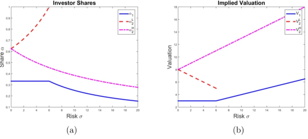
Figure 2 shows comparative statics for this simple model. Panel (a) shows the shares acquired in each period and state as a function of the risk (σ) of the underlying asset. Panel (b) shows the post-money valuation in each state as a function of the risk. It is easy to see that as long as reinvestment depends on the realization of the signal the value of the firm is increasing in the risk of the underlying asset.
Model Takeaways
The model formalizes the intuition that the real option to reinvest or abandon is valuable and that its value rises with the volatility of the underlying asset. Since the investor is perfectly competitive, the entrepreneur retains all of the surplus generated by the project, though in the real world one may expect either private information or other form of market power on the part of the investor to cause a more even split in surplus. Regardless, once the initial investment is made, any increase in the volatility of the assetσ will lead to an increased valuation for the investor.
Specifically, this simple model makes the time-series prediction that reinvestment options lead innovations to the level of asset volatility, after the initial investment and before the final invest-ment, to increase investment performance. This prediction is distinct from that of, for example, Ewens, Jones and Rhodes-Kropf (2013) who investigate the implications of a principal-agent prob-lem between investors and private equity firms. This friction drives a cross-sectional relationship between diversifiable risk and fund performance. These authors find that this relationship holds for both VC and buyout funds, as predicted by their model. Reinvestment options, in contrast, imply a time-series relationship only for VC firms, who retain reinvestment options, and not for buyout funds, who purchase going concerns.
3
Data Sources and Methodology
This section describes the data sources used in this paper. I use data on VC returns and investments at three levels of aggregation. First, I describe VC return indexes from Cambridge Associates (CA) and Sand Hill Econometrics (SHE), meant to proxy for the returns to investing in VC in aggregate. Second, I describe the private equity fund cash flow data from Burgiss. These are the realized cash flows experienced by investors into private equity funds. Third, I describe the investment-level data from the VentureSource database. These data describe the individual investments made by VC firms into their individual portfolio companies and the outcomes of these investments. I also describe construction of the measure of aggregate idiosyncratic volatility used throughout the paper and a measure of the level of idiosyncratic volatility of VC-backed portfolio companies.
3.1 Venture Capital Indexes
I use data on aggregate returns in the VC industry from Cambridge Associates and Sand Hill Econo-metrics. Cambridge Associates (CA) provides a quarterly net-of-fees VC returns series derived from disclosures by VC firm general partners. CA does not disclose what fraction of the universe of pos-sible investments their data cover. One potential concern with the CA VC return index is that it is subject to asynchronous prices resulting from the fact that VCs infrequently update (mark to market) the value of their portfolio holdings. This is due to the fact that fair (market) value of privately held companies is only observed when a new transaction for shares in the portfolio company takes place, at which point the valuation of previously held shares is adjusted.7 Those portfolio companies that do not experience a valuation event are left at the previous “stale” val-uation. This reporting convention causes net asset values, and therefore the returns reported by Cambridge Associates, to appear smoother and less correlated with market returns than are the unobservable true returns. This asynchronous trading problem has been studied by, for example, Lo and MacKinlay (1990) and Boudoukh, Richardson and Whitelaw (1994). Risk factors in the presence of asynchronous prices can be recovered by projecting returns on contemporaneous and lagged factor returns and summing the estimated coefficients (Dimson 1979). Woodward (2009) contains a detailed example of this mechanism at work in VC data and estimates risk loadings in the CA VC indexes. Section 4.1 describes the quantitative effect of this correction. Korteweg and Sorensen (2010) propose an alternative correction which I discuss in Section 3.5.
I use five different return indexes provided by Cambridge Associates. The first is meant to proxy for returns in the VC industry as a whole. Three other indexes are meant to proxy for returns of VC funds with different investment strategies: early-, multi- and late-focused VC funds. The final index proxies for the returns to buyout funds.
Sand Hill Econometrics (SHE) provides a monthly gross-of-fees return series derived from the individual VC investments (VentureSource, discussed below) rather than the net asset values re-ported by VC funds. SHE makes an effort to remove any bias introduced by asynchronous prices
7
In the VentureSource data, described below, the median (mean) time between consecutive financing rounds is 16 (21) months.
by interpolating values between rounds, using market indications of change in values. Details on SHE index construction are in Blosser and Woodward (2014).
3.2 Venture Capital Fund Cash Flow Data
VC fund performance data are from Burgiss, a global provider of investment decision support tools for the private capital market, and are described in detail by Harris, Jenkinson and Kaplan (2014). The Burgiss dataset contains the complete transactional history for over 6,800 private capital funds with a total capitalization representing over $4.7 trillion in committed capital across the full spectrum of private capital strategies. Kaplan and Lerner (2016) report that the Burgiss dataset is the likely the best available dataset of its type, with a non-selected sample and very high coverage. The Burgiss dataset is representative of actual investor experience, as the data are sourced exclusively from limited partners, avoiding any reporting biases introduced by sourcing data from general partner surveys. I focus my analysis on a sample of 914 VC funds first raised before 2011. Of these funds, 513 are designated as early stage funds, 118 as late stage funds and the remaining 283 are designated as balanced funds. Cash flows include draw-downs, flows from investors to VC funds, as well as distributions, flows from funds back to investors.
3.2.1 The Public Market Equivalent
The public market equivalent (“PME”), introduced by Kaplan and Schoar (2005), is a measure that evaluates fund performance based on cash flows. As discussed in Sorensen and Jagannathan (2015), which this discussion largely follows, the PME provides a valid economic performance measure when the investor (the limited partner or “LP”) has log-utility preferences and the return on the LPs total wealth equals the market return. When these conditions hold, the PME is a valid performance measure regardless of the risk of PE investments, and it is robust to variations in the timing and systematic risks of the underlying cash flows along with potential GP manipulations.
The PME calculation works as follows: LetX(t) denote the cash flow from the fund to the LP at timet. This cash-flow stream is divided into its positive and negative parts, called distributions,
dist(t), and capital capital draw-downs,draw(t). A distribution is a cash flow that is returned to the LP from the PE fund (net of fees) after the fund successfully sells a company. Capital
draw-downs are the investments by the LP into the fund, including management fees. Distributions and draw-downs are then discounted using the realized market returns over the same time periods, and the PME is the ratio of the two resulting valuations:
P M E= P t dist(t) 1+rM(t) P t draw(t) 1+rM(t) .
The sum runs over the life of the fund and rM(t) is the realized market return. A PME greater
than one suggests that the value of the distributions exceeds the cost of the capital calls, meaning the LP has benefited from the investment relative to the performance of the market.
3.3 Portfolio Company Data
Venture capital-backed company data are from the VentureSource database, maintained by Dow Jones. The full dataset contains 102,255 financing events for 30,689 companies, including seed, early, mezzanine and late round investments by VC firms, acquisitions by other companies and initial public offering (IPO) events. Most VC financings are syndicated, ie. involve more than one VC firm financing the company.
To calculate company-level investment returns requires data on exit valuation (either IPO or acquisition price) as well as the investment amount and fraction acquired for all rounds between the initial round and exit. Following the literature on investment-level VC returns, (e.g., Cochrane (2005), Korteweg and Sorensen (2010)), I calculate the gross multiple Mi,t as:
Mi,t = Vi VP ost i,t T Y s=t+1 Di,s,
whereT is the total number of dilutive financing rounds, Vi is the exit valuation,Vi,tP ost is the
post-money valuation for the round, and Di,s is the dilutive factor for each round, which is calculated
as 1−Ki,s/Vi,sP ost, whereKi,s is the total capital raised in financing round s.
As noted by Ewens, Rhodes-Kropf and Strebulaev (2016), investments that eventually have an initial public offering have a relatively higher probability of their valuation being reported. In contrast, acquisitions are much less likely to have prices and returns reported. As IPO returns tend
to exceed those of acquisitions, this leads to positive selection in any VC returns data. Conversely, acquisition returns are underrepresented in the sample of observed returns. I address this concern by following the Korteweg and Sorensen (2010) approach of re-weighting the observed returns using the true exit weights in the full sample.
3.4 Public Market Idiosyncratic Volatility
One potential concern with using idiosyncratic volatility to explain VC investment returns and investment dynamics is the fact that the idiosyncratic volatility of VC-backed firms may be en-dogenously determined by the amount of VC investment through, for example, an experimentation channel as argued by Nanda and Rhodes-Kropf (2013, 2016). For this reason, I construct a mea-sure from public market return data. Data on public equity market returns is from the Center for Research in Securities Prices (CRSP) as reported by Wharton Research Data Services (WRDS).
I construct a monthly measure of average idiosyncratic volatility that follows the measure doc-umented in Herskovic et. al. (2016). The Common Idiosyncratic Volatility (CIV) is constructed using data from the daily CRSP stock file for the years 1975-2014. Idiosyncratic returns are con-structed within each calendar monthτ by estimating a factor model using all observations within the month and takes the form:
rti=γiFt+εit
wheret denotes a daily observation in month τ. Idiosyncratic volatility for each firm is calculated as the variance of the residualsεi
twithin each month. The return factor model is purely statistical
and specifiesFtas a constant and the first five principal components of the cross section of returns
within the month. CIV is calculated as the equally-weighted average idiosyncratic volatility across firms.
I deviate from Herskovic et. al (2016) by measuring idiosyncratic volatility shocks as statistical innovations from the following ARMA(1,1) model on the level of CIV
whereas Herskovic et. al. (2016) construct CIV shocks as first-differences in the level of CIV, assuming a unit root. I estimate that the autoregressive coefficient ϕ is 0.936 and statistically different from unity (t= 3.85) and the moving average coefficientθ is -0.090 (t=−2.81).
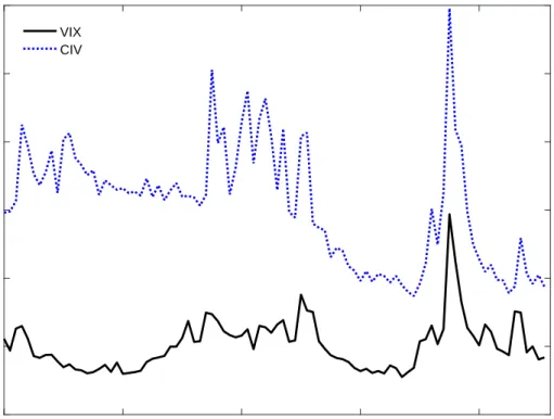
When regressions are at the quarterly or annual level, CIV shocks are measured as the average of the monthly CIV shocks over the quarter or year. Figure 3 shows quarterly CIV over time along with the VIX, a measure of systematic volatility. The correlation between the two series is 0.49 while the correlation between CIV shocks and similarly constructed VIX shocks is significantly lower (0.1).
3.5 Measuring Private Company Idiosyncratic Volatility
In order to validate the public market proxy (CIV) for the volatility of VC-backed firms, I compare low frequency estimates of the level of idiosyncratic volatility in these firms to similarly timed low frequency estimates from public markets. This section follows directly from Korteweg and Sorensen (2010); see their paper for details. These authors develop a Bayesian Markov Chain Monte Carlo estimation technique to estimate the risk and return characteristics of VC-backed company equity, incorporating a selection model to account for the fact that equity prices are observed infrequently and endogenously. This dynamic selection problem arises because valuations of these companies are observed only in the event that the company receives additional financing, either through a VC round or an initial public offering (IPO). They find that accounting for dynamic selection dramatically affects estimates of the market model parameters.
Korteweg and Sorensen (2010) address dynamic selection by simultaneously estimating the fol-lowing two-equation model:
v(t) = v(t−1) +r+δ+β(rm(t)−r) +ε(t) (2)
w(t) = Z0(t)γ0+v(t)γv+η(t) (3)
return and β is the factor loading on the market portfolio. They define δ =a−1 2σ 2+1 2β(1−β)σ 2 m (4)
where σ and σ2m are the variance of the asset and market return, respectively, andais the excess return of the asset. It is easy to see that a simple rearranging of equation 2 delivers something similar to the usual capital asset pricing model (CAPM).
Valuations are only observed when a company has an event and equation 3 captures this selection process. Valuation is only observed when the latent selection variablew(t) is greater than zero. The vectorZ(t) contains characteristics that affect refinancing and exit events and the error term η(t) is normalized to have variance of one. The estimation technique uses a Bayesian Gibbs sampling procedure to estimate the parameters of the model δ,β,σ2,γ0 and γv.
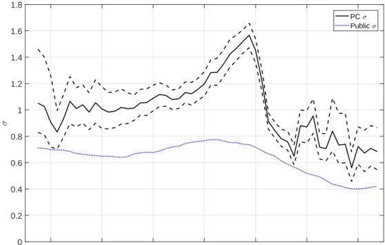
I use this method to estimate the level of idiosyncratic volatility (σ) in VC portfolio companies over time. Figure 4 shows these estimates along with 4-year averages of CIV. The horizontal axis represents the cohort being studied, with some overlap to smooth out the estimates. For example, the 1996Q2 cohort was first financed between January and September 1996. I estimate the idiosyncratic volatility of these firms until exit. The solid line represents the annualized idiosyncratic volatility of this cohort and the dashed lines represent the Bayesian confidence interval. Since the median VC-backed firm exits in about 4 years, I compare these estimates with average CIV over 4 years starting in the same quarter. The correlation between the two measures is 0.81, implying a substantial amount of commonality in the movement in idiosyncratic volatility between public and private markets. This result builds confidence in using a volatility measure derived from public equity markets.
4
Empirical Results
4.1 VC Industry Risk Exposures
I begin the empirical analysis by establishing that VC return indexes from two commonly used sources load on idiosyncratic volatility shocks. The first source is Cambridge Associates (CA) who
report a number of net-of-fees VC indexes meant to benchmark for the VC industry as a whole as well as those VCs with specific investment focuses. CA also reports a benchmark index for buyout funds. The second source is Sand Hill Econometrics who report a gross-of-fees VC return index meant to proxy for the returns VC firms themselves earn from their portfolio companies. I then discuss the implications for expected returns of VC investments if the price of volatility risk is non-zero.
4.1.1 Net-of-fees VC Index from Cambridge Associates
Regression results using the net-of-fees VC return indexes from Cambridge Associates are presented in Table 1. To see the effect of asynchronous prices empirically, consider the na¨ıve CAPM regression in column (1):
rtCA =α+βM(rmt −r f t) +εt.
We can see that the CAPM results imply that the market beta of VC is a small 0.47 and that the VC industry delivers a quarterly alpha of 2.58 percentage points. The problem with this result, as discussed in Section 3.1, is that the returns to VC as reported by CA are related both to contemporaneous and lagged market returns because of return smoothing and asynchronous prices. These features of VC portfolios lead to large serial correlation in the VC returns reported by CA.
We can address asynchronous prices by including lagged market returns in the regression as suggested by Dimson (1979): rCAt =α+X τ βτ(rmt−τ −r f t−τ) +εt.
For example, columns (2) and (3) of Table 1 report regression results including additional lags of the market return. The sum of the coefficient estimates is reported in the row labeledP
β. Here we can see that the lagged market returns enter with positive and statistically significant coefficients, indicating that VC industry returns depend on contemporaneous and lagged market returns because of asynchronous prices. The sum of the betas, representing the true market exposure, is 1.39 and the risk-adjusted alpha is close to zero, once we account for asynchronous prices. The largest and
most statistically significant lagged return coefficients are those on the 2-, 3- and 4-quarter lagged market returns.
To study the impact of idiosyncratic volatility shocks on VC returns, I additionally include contemporaneous and lagged CIV shocks to the regression:
rCAt −rft =α+X τ βτ(rmt−τ −r f t−τ) + X τ δτεCIVt−τ +εt. (5)
These shocks have been normalized to have a quarterly standard deviation of one. Column (4) of Table 1 reports results from this regression. The sum of the coefficient estimates on the CIV shocks is reported in the row labeledP
δ. We can see that past innovations in idiosyncratic volatility have a significant effect on VC returns as reported by CA. The sum of the coefficients on the idiosyncratic volatility shock in column (4) is 7.757, implying that a positive one-standard deviation shock to the level of idiosyncratic volatility corresponds to approximately an 8 percentage point return to VC investors. The row labeled “F” is the p-value from an F-test whose null hypothesis is that the sum of the coefficients on the CIV shock is zero, which we can easily reject at conventional levels. It is also interesting to note that the lagged CIV shocks with the largest and most statistically significant coefficients are those on the 2-, 3- and 4-quarter lagged shocks, similar to the lagged market return coefficients. The increase in theR2 between columns (3) and (4) is 0.104, implying that CIV shocks explain a substantial portion of the return variance not explained by the market. Note that, once I include the idiosyncratic volatility shocks in the return regressions, the regression intercept can no longer be interpreted as a return, since the CIV shocks are statistical innovations and not tradeable portfolios. See Section 4.1.3 below for a discussion of the implications for risk-adjusted expected returns.
The remaining columns in Table 1 report results for other return indexes reported by Cambridge Associates. Columns (5), (6) and (7) report results for indexes constructed from early-, balanced-and late-focused funds, respectively. While all three VC strategy indexes load significantly on the CIV shocks, the loading for the early-focused fund index is much larger than that for the balanced-or late-focused fund indexes (9.78 versus 3.69 and 4.81, respectively). Early-focused VC funds also
have a larger loading on the market return than late-focused funds. The final column in Table 1 reports results from the same regression where the dependent variable is now the benchmark return for leveraged buyout funds. In contrast to the results for VC indexes, the buyout index does not load significantly on CIV shocks.
To confirm that it is truly idiosyncratic volatility, rather than systematic volatility, driving the results I run untabulated regressions including contemporaneous and lagged measures of both CIV shocks and VIX shocks, where VIX shocks are measured as ARMA(1,1) innovations to the level of VIX. Shocks to the level of systematic volatility enter the regression insignificantly whether or not the regression includes CIV shocks. In contrast, shocks to CIV enter strongly significantly whether or not VIX shocks are included in the regressions.
4.1.2 Gross-of-fees VC Index from SHE
I also investigate the idiosyncratic volatility exposure of the VC return index from Sand Hill Econo-metrics (SHE). SHE provides a monthly, gross-of-fees VC return index that has been constructed to account for asynchronous prices as discussed in Blosser and Woodward (2014) and Woodward and Hall (2004). This series is constructed to measure the monthly return of a value-weighted portfolio of VC-backed companies, while the CA indexes discussed above are meant to represent averages of returns to investments in venture capital funds.
Factor regression results for this index are presented in Table 2. To establish a baseline for this index, column (1) shows the results for the Fama French 3-factor model. The SHE index has a large loading on the market return and a negative loading on the HML portfolio. While the contemporaneous CIV shock doesn’t enter significantly (column (2)), lagged CIV shocks do seem to be significantly related to VC returns as measured by this index (Columns (3) and (4)). While only a few of the lagged CIV shocks are significant individually, their sum is large and highly significant. The summed value of the lags is 1.69, implying that a one standard deviation monthly CIV shock is associated with a 1.69% return. The row labeled “F” is again the p-value from an F-test whose null hypothesis is that the sum of the lagged CIV coefficients is zero.
The fact that the lagged exposure of the SHE index to CIV shocks is positive indicates that the SHE procedure does not purge VC investment returns of their lagged exposure to idiosyncratic
volatility.
4.1.3 Implications for Expected Returns
The implications of volatility exposure for risk-adjusted VC returns depend on the price of id-iosyncratic volatility risk. Herskovic et. al. (2016) present evidence showing that the level of idiosyncratic volatility proxies for idiosyncratic income risk faced by households and thus argue that the price of volatility risk is negative, i.e. that investors are willing to accept lower returns for assets have positive return exposure to aggregate idiosyncratic volatility. This is because such an exposure would hedge their own exposure to idiosyncratic income risk. In this case the inclusion of this priced risk will increase the risk-adjusted expected returns of VC investments.
To test this hypothesis, I run a regression like that in Eq. (5) but using a tradeable portfolio that is exposed to the level of aggregate idiosyncratic volatility. I construct such a portfolio by taking an equally weighted position in 91-day straddle positions in S&P 500 constituents on the last trading day of each quarter. The construction of the option straddle portfolio is detailed in the appendix. This option portfolio delivers a mean return of -2.46% per quarter with a standard deviation of 21% for an annualized Sharpe ratio of -0.23. The average risk-adjusted return and Sharpe ratio are virtually unchanged in a Carhart (1997) four-factor model. Regression results are in Table 3. Since option prices on individual stocks are only available beginning in 1996, there are many fewer observations.
I start by re-running the analysis of Table 1 column (3) in column (1) of Table 3 to give a baseline for the estimates of market slope and intercept, which are both somewhat higher in this time period, relative to the estimates from the longer time period in Table 1. Column (2) adds the contemporaneous and lagged returns on the option straddle portfolio. The sum of coefficient estimates is a very statistically significant 0.70. Since the explanatory variables are all market returns, the intercept of the regression can be interpreted as a risk-adjusted excess return. Including the option straddle portfolio increases the intercept to a marginally significant 2.52% per quarter, which corresponds to an annualized increase of about 6% per year. In unreported regressions, I find that if CIV shocks are included in the regression along with returns on the option straddle portfolio, the loadings on the option portfolio returns become insignificant while the loadings on
the CIV shocks remain quite significant. This suggests that whatever explanatory power the option portfolio has is fully subsumed by the actual idiosyncratic volatility shocks.
Columns (3)-(5) repeat the analysis for early-, balanced- and late-focused VC funds respectively. The patterns are similar to those in Table 1 in that the coefficient estimates on the idiosyncratic volatility proxy are largest for the early-focused VC fund benchmark. Column (6) repeats the analysis for the buyout fund benchmark, which does not load significantly on the option portfolio return.
4.2 Investment Sample Results
To understand the impact of idiosyncratic volatility on individual VC investments, I next use the cash flows from individual VC funds. VC fund cash flow data has two large advantages over the industry indexes studied above. First, the funds are investment vehicles and the reported cash flows are the actual cash flows that investors receive. Given the illiquid nature of private equity funds, it is important to take the timing of cash flows into account. The second large benefit of using individual fund cash flows is that it allows an investigation into when, during a funds life, asset volatility shocks matter the most. This will in turn allow a better understanding of the mechanism driving this unique risk exposure.
I begin by regressing the PME on the average level and innovations to idiosyncratic volatility. The basic empirical specification is as follows:
P M Ei=α+βCIVi+i (6)
where P M Ei is calculated from quarterly fund cash flows and CIVi is a measure of the level of
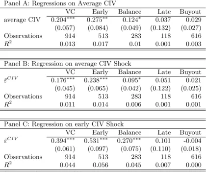
or innovation in CIV scaled by the cross sectional standard deviation. Results are in Table 4. Panel A reports results for regressions of PME on the average level of CIV over the fund life, from the month the fund was founded through the last cash flow has been distributed, an average of ten years. In the first column, labeled “VC”, the sample is VC funds covered by Burgiss. The positive and statistically significant coefficient implies that funds earn higher returns relative to public market equity when the level of CIV is higher over the life of the fund. The coefficient
of 0.204 implies that funds that experience lifetime idiosyncratic volatility one standard deviation above (the cross-sectional) average outperform public markets by over 20% more than average over the course of the fund’s life.
The other columns of panel A investigate the same regression in subsamples. VC funds in Burgiss are designated as early-, late- or balanced-focus funds, depending on what stage their portfolio companies are in when the funds first invest. We should expect idiosyncratic volatility exposure to be largest for those VC funds that invest in early-stage investments, since these funds are more likely to have reinvestment opportunities. The other columns in panel A show that this is indeed the case: the coefficient on average CIV for early stage funds is larger and more significant than for the other fund types. Late stage funds have an insignificant loading on average CIV, as do buyout funds.
Panels B and C of Table 4 show results for regressions of PME on average CIV shocks. CIV shocks are calculated as documented in section 3.4. In panel B, CIV shocks are averaged over the life of the fund. Results using CIV shocks averaged over the fund life are similar to those using level, which is reasonable considering the level reflects accumulated shocks. In particular, the pattern of early stage-focused VC fund performance being more exposed to idiosyncratic volatility remains. In unreported regressions, I include the initial level of CIV at fund initiation. This additional explanatory variable enters insignificantly, implying that any information about future expected volatility contained in the level is fully incorporated into the price of fund investments.
Private equity funds usually last for about 10 years. Therefore the idiosyncratic volatility shocks that I have investigated so far are averaged over those very long time periods. Panel C of Table 4 investigates the impact of idiosyncratic volatility shocks averaged over the 12th through 48th month of the fund’s life, the time when reinvestments are most likely to happen. The coefficient estimates and R2 are significantly higher when we focus on this period of the fund life. Focusing on the full VC sample (column 1), I find that funds that experience idiosyncratic volatility one standard deviation above (the cross-sectional) average in years two through four of fund life outperform public markets by almost 40% more that average over the course of the fund’s life. This rises to 53% when we consider the subsample of early-focused funds. This is equivalent to an annual return
of 4.3% over a ten year fund. The R2 for this sample implies that the time-series of CIV shocks explains over 5% of the cross-sectional variance of early-focused VC funds.
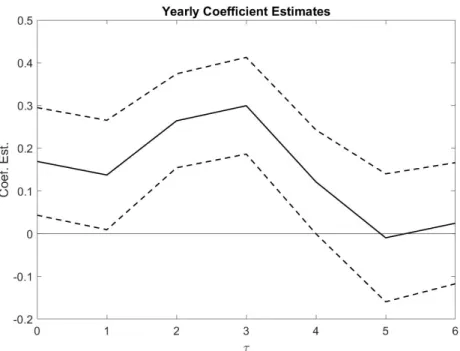
For a more granular look, I next regress VC fund performance on multiple CIV shocks, one for each of the first seven years the fund was in operation. To build these shocks, I average the monthly CIV shock across each fund year. For example, if a fund was first raised in June 1995, the first CIV shock is measured as the average monthly CIV shock from July 1995 through June 1996, the second is from July 1996 through June 1997, etc. The explanatory variables are again scaled so that one is equivalent to a single cross-sectional standard deviation. Results are in Figure 5 which shows coefficient estimates and 95% confidence bounds on these estimates. We can see that the impact of CIV shocks starts positive and marginally statistically significant, is highest and highly significant in years 3 and 4 of the funds life, and falls close to zero by year 6. Together these results suggest that CIV shocks help explain VC fund performance and that this effect is stronger during the period when VC funds are likely to have already made investments and to be exercising reinvestment options.
I next ask what the implication of these fund-level regression results is for the time-series of VC fund performance. Using the same Burgiss dataset that underlies this section, Harris, Jenkinson and Kaplan (2014) find that “Average VC fund returns in the United States [...] outperformed public equities in the 1990s but have underperformed public equities in the most recent decade.” Korteweg and Sorensen (2010) document a similar pattern in the returns of VC-backed companies. Accounting forex-post realized shocks to the aggregate level of idiosyncratic volatility can help to explain these patterns.
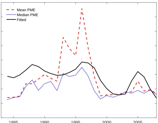
Figure 6 shows mean and median fund performance, as measured by PME, along with the pre-dicted performance given realized CIV shocks. The dashed (red) line is the mean fund performance and the dotted (blue) line is the median fund performance for funds within each vintage cohort. The mean is generally higher than the median due to the skewed performance of VC funds. Vin-tage year is defined by the date of the first fund cash flow. These realized performance measures, solid black line, are matched with fitted performance measures from regression Equation 6 where the measure of CIV used is average over the 12th through 48th month as in Panel C of Table 4.
The fitted performance demonstrates that, given the ex-post realized CIV shocks, the difference in relative performance over time is not as large as previously believed.
4.2.1 Alternativeβ benchmarks
One potential concern with the PME measures introduced in section 3.2.1 and used in section 4.2 is that the relevant benchmark for VC funds may not be a market index with a β of unity. To address this concern, I repeat the analysis or section 4.2 using market benchmarks with different levels of market exposure. Results are in Table 5 and indicate that the broader pattern remains no matter what β benchmark is used.
4.3 Portfolio Company Sample Results
The final data set I investigate is Dow Jones VentureSource, discussed in Section 3.2. I focus on a sample of 111,766 investments by 1,615 VC firms into 19,638 individual portfolio companies made between 1990 and 2011. There are 47,411 financing events, most of which involve more than one investor. I require a VC firm to participate in at least ten financing rounds to enter the sample. I match these financing events with public market condition. Public market data are from the web page of Kenneth French and CRSP. Corporate accounting data are from Compustat. To measure average market prices of public firms I calculate an average measure of Tobin’sq that incorporates intangible assets in the denominator from Peters and Taylor (2016). Market returns (rt,tm+1) are value weighted and measured over the following year and are calculated using the CRSP universe. Summary Statistics are presented in Table 6.
The variablesIP Oand DEF are indicators for whether the company has had a successful IPO or default respectively. A company is identified as having defaulted if it is listed as out of business, in bankruptcy, or has been otherwise identified by VentureSource as not active. A company is also labeled as having defaulted if it received the first VC funding prior to 2004, has yet to exit by the end of the sample, and has never had a successful exit event. I designate a round as an early stage investment if VentureSource identifies the round as being either a seed, angel or first round and a late stage round otherwise, 29.2% of the sample. The variable ‘supply” is the quarterly flow of capital into the VC sector as reported by the National Venture Capital Association (NVCA). In all
regressions in this section,CIVt and Qtare measured at the date of financing, εCIVt,t+1 is the sum of monthly CIV shocks over the year following the first financing andrt,tm+1 is the market return over this same period.
I begin my analysis of company-level data with a consistency check: do firms funded in times of high idiosyncratic volatility experience more extreme investment outcomes? To investigate this question I identify extreme outcomes as a firm having either an observed default or an IPO. Table 7 regresses these firm outcomes on various firm characteristics and aggregate conditions. The dependent variable in columns (1)-(3) is an indicator for firm default, and coefficient estimates are expressed in percentage points. Column (1) regresses this variable on the level of CIV at the first financing round, the Industry Q of small, high-tech firms in the quarter of financing, and innovations to both the level of CIV and market price. The coefficient estimates indicate that companies first financed in times of high prices and high idiosyncratic volatility are more likely to default. Column (2) includes a number of company-level control variables: The firm age at first financing as reported by VentureSource, the size of the investing syndicate, the log dollars raised and whether the company is based in California or Massachusetts. Including these variables does not qualitatively impact the result. Column (3) adds industry fixed effects to the regression, which does not change the results appreciably.
Columns (4)-(6) of Table 7 studies the effect of market conditions at first financing on firms’ probability of successfully completing an IPO. This is generally considered the best outcome for a VC-backed company. The dependent variable is an indicator for whether the firm has a successful IPO, again expressed in percentage points. Column (4) shows that firms first financed in high CIV times are more likely to successfully IPO. Interestingly, average stock prices (at time of first financing) do not seem to greatly impact the probability that VC-backed firms successfully IPO, implying that the increase observed in columns (1)-(3) comes primarily from a decrease in the number of firms acquired. Finally, firms first financed in times of high VC fund supply are markedly less likely to successfully IPO. Including additional firm-level controls and industry fixed effects, as in columns (5) and (6) do not change these results.
in-vestment process. Table 8 reports results for regressions on the frequency of reinin-vestment. The dependent variable is an indicator for whether the same VC firm has a follow-on investment after the round. In general, VC financing relationships are stable in the sense that the same VC firm will usually continue to finance the firm after making an initial investment. The results in Columns (1)-(3) of Table 8 indicate that rising idiosyncratic volatility (εCIVt,t+1) and market prices (rt,tm+1) after the financing round are associated with a greater probability of their being a follow-on financing event from the same VC firm. Columns (4)-(6) and (7)-(8) repeat the analysis in early and late rounds, respectively, where early rounds are those that VentureSource has Identified as being seed, angel or first rounds of investments. In general, early investment rounds are more likely to be in-volve follow-on investments (65% vs. 52%) and the results in Table 8 imply that these probabilities are also more strongly related to public market conditions. A one-standard-deviation movement in idiosyncratic volatility is associated with a 4% greater probability of follow-on financing for early rounds, while the probability of follow-on financing does not change for late financing rounds. Mar-ket returns also have a greater impact on early financing rounds, with a one standard deviation move in market prices associated with a 6% change in the probability of follow-on financing for early rounds and only a 1.3%-1.9% change in later rounds.
Table 9 investigates whether, conditional on there being a follow-on financing round, how does the time until that round relate to any changes in underlying asset volatility. The dependent variable, time until the next financing round, is measured as the natural logarithm of the number of days until the next round. The results imply that, conditional on a new financing round occurring, the round is significantly faster in times of rising asset volatility as well as in times of rising market prices.
Finally, I investigate whether realized asset volatility shocks are correlated with returns for individual portfolio company investments. In the theoretical motivation in Section 2, the presence of a reinvestment option implies that the returns should depend on innovations to idiosyncratic volatility after the company is first financed, and not on thelevel of idiosyncratic volatility at the time of financing. To test this hypothesis, I regress gross cash multiples on levels and innovations
of both CIV and market prices:
Mi,t =γ0+γ1CIVt+γ2εCIVt,t+1+γ3Qt+γ4rmt,t+1+δX+ηi,t.
The variableX is a potential vector of company characteristics and fixed effects.
Results for this regression are in Table 10. Starting with column (1), which does not include firm-level controls or fixed effects, we can see that the coefficient on the level of CIV at first financing enters insignificantly, consistent with the theoretical motivation. The level of asset volatility appears to be priced into portfolio company investments, consistent with competitive financing markets. The innovation to CIV (εCIVt,t+1), on the other hand, enters positively and significantly. Market prices enter similarly, with the coefficient Tobin’s Q entering with only marginal significance and market returns after the investment strongly statistically significant. Columns (2) and (3) include company-level controls and industry fixed effects, neither of which materially impact these results dramatically. Columns (4)-(6) and (7)-(9) repeat the analysis in early and late rounds, respectively. Similar to the results reported in Sections 4.2 and 4.3, the return of early-stage investments are much more strongly related to innovations in asset volatility than those for late investment rounds.
5
Conclusion
The contractual arrangements through which VC firms invest in their portfolio companies, in par-ticular the real option embedded in staged financing, lead these funds to be exposed to changes in the idiosyncratic volatility of these companies. The idiosyncratic return volatility of these com-panies is, in turn, exposed to aggregate levels of idiosyncratic volatility through a common factor structure. I find that this channel explains a significant fraction of the historical performance of VC investments.
At the asset class level, VC indexes from Cambridge Associates and Sand Hill Econometrics show significant exposure to idiosyncratic volatility shocks, with a one standard deviation quarterly shock leading to an 8% return in the CA index. This loading is even larger for a benchmark index of early stage investment focused funds and is smaller for balanced- and late-focused funds. An index
of buyout funds shows no exposure to idiosyncratic volatility shocks. I repeat the analysis using a tradeable proxy for idiosyncratic volatility shocks constructed from equity options and find that the exposure to this proxy increases risk-adjusted excess returns. One possible interpretation of this result is that investors who ignore this valuable risk exposure undervalue the returns to venture capital investments.
At the investment level, I find that positive innovations to idiosyncratic volatility that occur during the fund’s life lead to greater fund performance relative to a market benchmark, and that the shocks with the greatest impact are those that occur in years three and four of the fund’s life. Again, funds that focus on early-stage investments, i.e. those with more reinvestment options, experience much greater performance exposure to idiosyncratic volatility shocks.
At the level of individual portfolio company investments, I find that the average cash multiple is greater for those investments that experience positive innovations to idiosyncratic volatility early in their lives, but that the level of idiosyncratic volatility does not predict returns, consistent with rational and competitive pricing in the market for entrepreneurial finance.
REFERENCES
Ang, A., Hodrick, R.J., Xing, Y. and Zhang, X., 2006. The crosssection of volatility and expected returns. The Journal of Finance, 61(1), pp.259-299.
Bergemann, D. and Hege, U., 1998. Dynamic venture capital financing, learning and moral hazard. Journal of Banking and Finance, 22(6-8), pp.703-735.
Bergemann, D. and Hege, U., 2005. The financing of innovation: Learning and stopping. RAND Journal of Economics, pp.719-752.
Biais, B., Mariotti, T., Plantin, G. and Rochet, J.C., 2007. Dynamic security design: Convergence to continuous time and asset pricing implications. The Review of Economic Studies, 74(2), pp.345-390.
Black, B.S. and Gilson, R.J., 1998. Venture capital and the structure of capital markets: banks versus stock markets. Journal of financial economics, 47(3), pp.243-277.
Black, F. and Scholes, M., 1973. The pricing of options and corporate liabilities. The journal of political economy, 81(3), pp.637-654.
Blosser, S. and Woodward, S.E., 2009. VC index calculation white paper. Available at http://www.sandhillecon.com/pdf/SandHillIndexWhitePaper.pdf
Boudoukh, J., Richardson, M.P. and Whitelaw, R.F., 1994. A tale of three schools: Insights on autocorrelations of short-horizon stock returns. Review of financial studies, 7(3), pp.539-573. Campbell, J.Y., Lettau, M., Malkiel, B.G. and Xu, Y., 2001. Have individual stocks become more
volatile? An empirical exploration of idiosyncratic risk. The Journal of Finance, 56(1), pp.1-43. Carhart, M.M., 1997. On persistence in mutual fund performance. The Journal of finance, 52(1),
pp.57-82.
Cochrane, J.H., 2005. The risk and return of venture capital. Journal of financial economics, 75(1), pp.3-52.
Constantinides, G.M. and Duffie, D., 1996. Asset pricing with heterogeneous consumers. Journal of Political economy, pp.219-240.
Cornelli, F. and Yosha, O., 2003. Stage financing and the role of convertible securities. The Review of Economic Studies, 70(1), pp.1-32.
Da Rin, M., Hellmann, T. F., and Puri, M. (2011). A survey of venture capital research (No. w17523). National Bureau of Economic Research.
DeMarzo, P.M. and Fishman, M.J., 2007. Optimal long-term financial contracting. Review of Financial Studies, 20(6), pp.2079-2128.
DeMarzo, P.M. and Sannikov, Y., 2006. Optimal Security Design and Dynamic Capital Structure in a ContinuousTime Agency Model. The Journal of Finance, 61(6), pp.2681-2724.
Dimson, E., 1979. Risk measurement when shares are subject to infrequent trading. Journal of Financial Economics, 7(2), pp.197-226.
Engle, R. and Figlewski, S., 2015. Modeling the dynamics of correlations among implied volatilities. Review of Finance, 19(3), pp.991-1018.
Ewens, M., Jones, C.M. and Rhodes-Kropf, M., 2013. The price of diversifiable risk in venture capital and private equity. Review of Financial Studies, 26(8), pp.1854-1889.
Ewens, M., Rhodes-Kropf, M. and Strebulaev, I., 2016. Inside rounds and venture capital returns. Unpublished Working Paper
Fluck, Z., Garrison, K. and Myers, S.C., 2006. Venture capital contracting: Staged financing and syndication of later-stage investments. NBER Working Paper.
Gompers, P.A., 1995. Optimal investment, monitoring, and the staging of venture capital. The journal of finance, 50(5), pp.1461-1489.
Hall, R.E. and Woodward, S.E., 2007. The incentives to start new companies: Evidence from venture capital (No. w13056). National Bureau of Economic Research.
Hall, R.E. and Woodward, S.E., 2010. The burden of the nondiversifiable risk of entrepreneurship. The American Economic Review, 100(3), pp.1163-1194.
Harris, R.S., Jenkinson, T. and Kaplan, S.N., 2014. Private equity performance: What do we know?. The Journal of Finance, 69(5), pp.1851-1882.
Heaton, J. and Lucas, D., 2004. Capital structure, hurdle rates, and portfolio choice interactions in an entrepreneurial firm. Unpublished working paper. University of Chicago and Massachusetts Institute of Technology.
Hellmann, T. and Puri, M., 2000. The interaction between product market and financing strategy: The role of venture capital. Review of Financial studies,13(4), pp.959-984.
Hellmann, T. and Puri, M., 2002. Venture capital and the professionalization of startup firms: Empirical evidence. The journal of finance, 57(1), pp.169-197.
Herskovic, B., Kelly, B., Lustig, H. and Van Nieuwerburgh, S., 2016. The common factor in id-iosyncratic volatility: Quantitative asset pricing implications. Journal of Financial Economics, 119(2), pp.249-283.
Jurado, K., Ludvigson, S.C. and Ng, S., 2015. Measuring uncertainty. The American Economic Review, 105(3), pp.1177-1216. Vancouver
Kaplan, S.N. and Lerner, J., 2016. Venture Capital Data: Opportunities and Challenges (No. w22500). National Bureau of Economic Research.
Kaplan, S.N. and Schoar, A., 2005. Private equity performance: Returns, persistence, and capital flows. The Journal of Finance, 60(4), pp.1791-1823.
Kaplan, S.N. and Strmberg, P., 2003. Financial contracting theory meets the real world: An empirical analysis of venture capital contracts. The Review of Economic Studies, 70(2), pp.281-315.
Korteweg, A. and Nagel, S., 2016. Riskadjusting the returns to venture capital. The Journal of Finance, Forthcoming.
Korteweg, A. and Sorensen, M., 2010. Risk and return characteristics of venture capital-backed entrepreneurial companies. Review of Financial Studies, 23(10), pp.3738-3772.
Lerner, J., 1995. Venture capitalists and the oversight of private firms. The Journal of Finance, 50(1), pp.301-318.
Lo, A.W. and MacKinlay, A.C., 1990. An econometric analysis of nonsynchronous trading. Journal of Econometrics, 45(1-2), pp.181-211.
Mankiw, G.N., 1986. The equity premium and the concentration of aggregate shocks. Journal of Financial Economics 17, pp.211219.
Merton, R.C., 1973. Theory of rational option pricing. The Bell Journal of economics and man-agement science, 4(1), pp.141-183.
Metrick, A., and Yasuda, A., 2011. Venture capital and the finance of innovation, 2nd Edition, John Wiley and Sons, Inc.
Nanda, R. and Rhodes-Kropf, M., 2013. Investment cycles and startup innovation. Journal of Financial Economics, 110(2), pp.403-418.
Nanda, R. and Rhodes-Kropf, M., 2016. Financing Risk and Innovation. Management Science, Forthcoming.
Peters, R.H. and Taylor, L.A., 2016. Intangible capital and the investment-q relation. Journal of Financial Economics, Forthcoming.
Sorensen, M. and Jagannathan, R., 2015. The public market equivalent and private equity perfor-mance. Financial Analysts Journal, 71(4), pp.43-50.
Woodward, S.E., 2009. Measuring risk for venture capital and private equity portfolios. Available at SSRN 1458050.
Woodward, S.E. and Hall, R.E., 2004. Benchmarking the returns to venture (No. w10202). Na-tional Bureau of Economic Research.