Understanding, Modeling and Managing Longevity Risk:
Key Issues and Main Challenges
Pauline Barrieu, Harry Bensusan, Nicole El Karoui, Caroline Hillairet,
St´
ephane Loisel, Claudia Ravanelli, Yahia Salhi
To cite this version:
Pauline Barrieu, Harry Bensusan, Nicole El Karoui, Caroline Hillairet, St´
ephane Loisel, et al..
Understanding, Modeling and Managing Longevity Risk: Key Issues and Main Challenges.
Scandinavian Actuarial Journal, Taylor & Francis (Routledge), 2012, 2012 (3), pp.203-231.
<
hal-00417800v2
>
HAL Id: hal-00417800
https://hal.archives-ouvertes.fr/hal-00417800v2
Submitted on 16 Jul 2010
HAL
is a multi-disciplinary open access
archive for the deposit and dissemination of
sci-entific research documents, whether they are
pub-lished or not.
The documents may come from
teaching and research institutions in France or
abroad, or from public or private research centers.
L’archive ouverte pluridisciplinaire
HAL
, est
destin´
ee au d´
epˆ
ot et `
a la diffusion de documents
scientifiques de niveau recherche, publi´
es ou non,
´
emanant des ´
etablissements d’enseignement et de
recherche fran¸
cais ou ´
etrangers, des laboratoires
publics ou priv´
es.
Understanding, Modelling and Managing Longevity Risk: Key Issues
and Main Challenges
1Pauline Barrieua, Harry Bensusanb, Nicole El Karouib, Caroline Hillairetb, St´ephane Loiselc,
Claudia Ravanellid, Yahia Salhic,e a Statistics Department - London School of Economics
bCMAP - ´Ecole Polytechnique cISFA - Universit´e Claude Bernard Lyon 1 d Ecole Polytechnique F´ed´erale de Lausanne eR&D Longevity-Mortality - SCOR Global Life
Abstract
This article investigates the latest developments in longevity risk modelling, and explores the key risk management challenges for both the financial and insurance industries. The article discusses key definitions that are crucial for the enhancement of the way longevity risk is understood; providing a global view of the practical issues for longevity-linked insurance and pension products that have evolved concurrently with the steady increase in life expectancy since 1960s. In addition, the article frames the recent and forthcoming developments that are expected to action industry-wide changes as more effective regulation, designed to better assess and efficiently manage inherited risks, is adopted. Simultaneously, the evolution of longevity is intensifying the need for capital markets to be used to manage and transfer the risk through what are known as Insurance-Linked Securities (ILS). Thus, the article will examine the emerging scenarios, and will finally highlight some important potential developments for longevity risk management from a financial perspective with reference to the most relevant modelling and pricing practices in the banking industry.
Key words: Longevity risk, stochastic mortality, pensions, life insurance, regulation, long-term
interest rates, securitisation, risk transfer, incomplete market, population dynamics.
The sustained improvements in longevity currently observed, are producing a considerable num-ber of new issues and challenges at multiple societal levels. This is causing pensions to be one of the most highly publicised industries to be impacted by rising longevity. In 2009 many companies based in developed countries had closed the defined benefit retirement plans previously offered to their employees (such as the 401(K) pension plans in the United States). Broadly speaking, such scheme trends indicate a risk transfer from both the industry and the insurers, back to the policyholders, which from a social point of view is no longer satisfactory. Similarly, in several countries, defined benefit pension plans have continued to be replaced with defined contribution plans, which will most likely lead to the same result. Furthermore, a number of governments are set to increase retirement ages by 2 to 5 years to be able to take into account the changing dynamics of longevity improvements, and the impacts of ageing populations upon the financing of pensions.
The insurance industry is also facing a number of specific challenges related to longevity risk (i.e. the risk that trends in longevity improvements will change significantly in the future). In practical terms, greater capital has to be constituted to balance the long-term risk, a requirement only reinforced
1We are grateful to an anonymous referee for his valuable comments. We also thank the F´ed´eration Bancaire Fran¸caise for its financial support to the working group on longevity risk.
by the impacts of the financial crisis and new European regulation. Consequently, it has become paramount for insurance companies and pension funds to find a suitable and efficient way to cross-hedge, or to transfer part of the longevity risk to reinsurers and the financial markets. However, in the absence of both theoretical consensus and established industry practices, the transfer of longevity risk is a difficult process to understand; and therefore, manage. In particular, because of the long-term nature of the risks, accurate longevity projections are delicate, and modelling the embedded interest rate risks remains challenging.
Prospective life tables containing longevity trend projections are frequently used to better manage longevity risk, proving to be particularly effective in reserving in life insurance. However, the irregu-larity of table updates can cause significant problems. For example, consider the French prospective life tables were updated in 2006; replacing the previous set of tables from 1993. The resulting dispar-ities between the 1993 prospective tables and observed longevity caused French insurers to sharply increase their reserves by an average of 8%. In addition, insurance companies and pension funds are facing basis risk as the the evolution of policyholder mortality is thought to differ form that of the national population as a result of selection effects. These selection effects may have different impacts on different portfolios, since the pace of change and levels of mortality are highly heterogeneous in the insurance industry, which makes it hard for insurance companies and pension funds to rely on national (or even industry) indices to manage their own longevity risk.
To better understand longevity risk, its dynamics, causes, and the aforementioned heterogeneity of longevity improvements must be studied carefully, and aside from shorter-term managerial oscillations concerning average trends. Among the many standard stochastic models for mortality, a number have been inspired by the classical credit risk and interest rate literature, and as such produce a limited definition of mortality by age and time. An alternative is the microscopic modelling approach, which can be used for populations where individuals are characterised not only by age, but also by addi-tional indicators that are reflective of lifestyle and living conditions. Such models can provide useful benefits for the risk analysis of a given insurance portfolio. Furthermore, when combined with studies on demographic rates, such as fertility and immigration, microscopic modelling is highly applicable at social and political levels, offering guidance for governmental strategies concerning, for example, immigration and retirement age policy.
The need to carry out microscopic studies is all the more apparent when the size of the considered portfolio is small and in all likelihood highly heterogeneous. This has proven particularly true when looking at the life settlement market (i.e. when owners of a life insurance policy sell an unneeded policy to a third party for more than its cash value and less than its face value). Although this market phenomenon carries anecdotal significance, it will not be studied specifically here. Rather, this paper focuses on longevity risk for the larger portfolio, often referred to as macro-longevity risk.
The European insurance industry will soon be expected to comply to the new Solvency II Directive. The regulatory standards of the directive place emphasis on the manner in which insurance company endorsed risk should be handled so that it can withstand adverse economic and demographic situations. The regulation is scheduled to come into effect by late 2012, and will certainly enhance the devel-opment of alternative risk transfer solutions for insurance-risk generally, as well as for longevity-risk in particular. There is little doubt that the pricing methodologies for insurance related transactions, and specifically longevity-linked securities will be impacted as greater numbers of alternative solutions appear in the market. Today, the longevity market is immature and incomplete, with an evident lack of liquidity. Standard replication strategies are impossible, making the classical financial methodology unapplicable. In this case, indifference pricing, involving utility maximisation, seems to be a more appropriate strategy. In any case, due to the long maturities of the underlying risk, the modelling of long term interest rates is unavoidable, adding to the complexity of the problem.
The following paper is organised as follows: Section 1 provides an outline of the main characteristics of longevity risk, focusing on the classical and prospective life tables, mortality data, and specific features such as the cohort effect and basis risk. Section 2 presents the key models for mortality-risk, discussing how they can be used to model longevity-risk. Section 3 is dedicated to longevity risk management in reference to the new solvency regulations that stand to be enforced by 2012. Section 4 centres on longevity risk transfer issues, and the convergence between the insurance industry and capital markets. The final section looks at a number of key modelling questions concerning the pricing of longevity risk.
1. Main characteristics of longevity risk
In this section, the main characteristics of longevity risk are outlined according to available data and important longevity and mortality risk related issues.
1.1. Age, period and cohort life tables and available mortality data
The analysis of mortality of a given population or insured portfolio can take multiple forms, depending on the purposes of the study, the data available, and its reliability. For such analysis, the period life and cohort life tables have proven to be most useful. The Lexis diagram in Figure 1.1 is an age-period-cohort diagram; the x-axis features calendar years and the y-axis corresponds to age. This representation enables the statistical understanding of both cohort and period life tables. Cohort life tables may be obtained from the diagonals of the Lexis diagram; period life tables are given by vertical bands. Both continuous and discrete-time analysis are feasible, the latter being most applied to national data, since the mortality of national populations is generally described by yearly observations2. The equivalence between discrete and continuous methods is based upon the
assumption that the mortality force (i.e. instantaneous mortality hazard rate) is constant (or does not fluctuate too much) within each square on the Lexis diagram.
However, the assumption of constant yearly mortality has to be avoided when observations of mortality are deeper than at a national level. Life insurers typically collect data for insured portfolios that are more accurate and that gives the actual ages attained by each insured individual. Thus, actuaries are used to derive the underlying mortality of such portfolios, taking into account censored observations, using the Kaplan-Meier estimator (see Klein and Moeschberger (2003)). It is therefore possible to build time-continuous life tables.
The difference between national mortality data and that of an insured portfolio is not only limited to the continuity of observations. First of all, one key difference between national mortality and specific mortality in some insured portfolios, is the range of the observation period. The period for which observed mortality rates for the insurance portfolio are available is usually limited, often in the range of only 5 to 15 years. In contrast, national data can range from 100 to 200 years (see the HMD databases for example). This is one of the main reasons why in order to determine the actual level and the future trend of mortality, actuaries and practitioners are used to model the national mortality and then to project the insured ones. One example of how such projections are produced is by relational models: a technique that aims at linking together both mortality rates and their future evolution, even if socio-economic variables cause the insurance portfolio specific mortality and the national mortality to differ.
In addition, at the portfolio level, whilst the movements in the group of policyholders are known and
2The available mortality data is based upon statistics coming from various national institutes (Including but not limited to: Bureau of Census in the US, CMI in the UK, INSEE in France). For most developed countries, this data is also available through the Human Mortality Database.
can be taken into consideration, it proves difficult to account for censured and truncated data when assessing national mortality. One may think for instance of migration. There are two different factors that can be overlooked when considering migratory impacts. First of all, people leaving the synthetic cohort are often censored, and thus still taken into account when estimating the period life tables. Secondly, incoming immigrants can also affect and significantly change the local national mortality data of the destination country.
Far more relevant details regarding deaths can be gained from within an insured portfolio (e.g. the cause of death). Although national data by cause of death does exist, it generally lacks consistency, and is often useless, or of no specific interest in deriving mortality by cause (for example: in the United States, 11% of deaths are caused by more than four diseases).
Cohort
Year
Age
66
65
64
63
2008
1943
1942
Figure 1.1: Lexis diagram: Age-year-cohort diagram.
1.2. Heterogeneity, inter-age dependence and basis risk
It is expected that any given population will display some degree of heterogeneous mortality. Heterogeneity often arises due to a number of observable factors, which include age, gender, occupation and physiological factors. As far as longevity risk is concerned, policyholders that are of higher socio-economic status (assessed by occupation, income or education) tend to experience lower levels of mortality. However, significant differences also exist within the same socio-economic levels according to gender. Females tend to outlive males and have lower mortality rates at all ages. In addition, some heterogeneity arises due to features of the living environment, such as: climate, pollution, nutritional standards, population density and sanitation (see Section 2.2 for a more detailed discussion). When considering insured portfolios, insurers tend to impose selective criteria that limits contractual access to those considered to possess no explosive risk (by level of health and medical history). This
induces differences in mortality profiles within different portfolios. For example, term and endowment assurance portfolios are experiencing higher mortality rates than those related to annuity portfolios and pensions. Also, the risks underlying those two types of contracts are different in nature. The resulting risk for the prior portfolios is a mortality risk, whilst the latter types have a longevity risk. By virtue of their opposing nature, the possibility remains for a hedge that implies both types of risk3.
However, as highlighted by Cox and Lin (2007), this natural hedge is only partial. The hedging is only partially attainable due to the nature of both risks and the different age ranges implied in the two specific contracts. In particular, the interdependence among ages, and even the inter-temporal correlation are dynamically significant and need to be understood.
In Loisel and Serant (2007), both the issue of inter-age dependency according to the mortality data and the inter-temporal correlation are considered. In this study, the population data for both males and females exhibits a clear dependence upon mortality rates among ages. This inter-age dependency is crucial when dealing with, for example, the natural hedge between mortality and longevity. More precisely, it gives a clear view of how some changes in mortality for a specific age-range will affect another by providing measurements of the associated liabilities altered by potential diversification due to inter-age correlation. Thus, it is a characteristic of considerable interest and importance when aggregating the benefits within a book of contracts.
2. Modelling longevity risk
In the previous section a detailed description of longevity risk and the available data has been presented. The next section will discuss the implications and issues of modelling, outlining some key methods that can be used to take into account relevant characteristics.
2.1. Some standard models
In recent years a variety of mortality models have been introduced, including the well known (Lee and Carter (1992)), widely used by insurance practitioners. The Renshaw-Haberman model (Renshaw and Haberman (2006, 2003)) was one of the first to incorporate a cohort effect parameter to characterise the observed variations in mortality among individuals from differing cohorts. For a detailed survey on the classical mortality models, Pitacco (2004) is referred to. In recent contemporary studies, many authors have introduced stochastic models to capture the cohort effect (see e.g. Cairns et al. (2006, 2009)); this subsection, briefly presents some of them.
The Lee-Carter model. The Lee Carter model describes the central mortality ratemt(x) or the force
of mortality,µx,t at agexand timetby 3 series of parameters namelyαx,βxandκt, as follows:
logµx,t=αx+βx·κt+εx,t, εx,t∼ N(0, σ),
whereαx gives the average level of mortality at each age over time, the time varying component κt
is the general speed of mortality improvement over time, and βx is an age-specific component that
characterises the sensitivity toκtat different ages; the βx also describes (on a logarithmic scale) the
deviance of the mortality from the mean behaviour κt. The error term εx,t captures the remaining
variations.
To enforce the uniqueness of the parameters, some constraints are imposed: X
βx= 1 and
X
κt= 0.
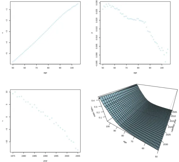
Some relevant extensions of this approach have also been proposed, incorporating, for example, the cohort effect as in Renshaw and Haberman (2006) or Haberman and Renshaw (2006). Meanwhile, given the high variability of the force of mortality at higher rather than at younger ages (due to a much smaller absolute number of deaths at older ages), the error term cannot be regarded as being correctly described by a white noise. Brouhns et al. (2005) has proposed an extension of the general framework by assuming the number of deaths to be a Poisson distribution. To calibrate the various parameters, standard likelihood methods can be applied, and a Poisson distribution can be considered for the number of deaths at each age over time. The estimated parameters are presented on Figure 2.1. It is important to note that estimated values forβtare higher at younger ages, meaning that at those
ages, the mortality improvements occur faster and deviate considerably from the evolutionary mean. In addition to the Lee and Carter (1992) model, similar models have been introduced to forecast mortality. For instance, the Cairns et al. (2006) two-factor model includes two time dependent com-ponents rather than a unique component as seen in the original Lee & Carter model. This model could be thought of as a compromise between the generalised regression approach and the Lee & Carter method. In addition, this approach allows components relevant to the cohort effect to be incorporated (for further details see Cairns et al. (2009)).
50 60 70 80 90 100 −5 −4 −3 −2 −1 age α 50 60 70 80 90 100 −0.005 0.000 0.005 0.010 0.015 0.020 0.025 0.030 age β 1975 1980 1985 1990 1995 2000 2005 −10 −5 0 5 10 year κ age 50 60 70 80 90 100 calendar year 2005 2010 2015 2020 2025 2030 mortality rates 0.1 0.2 0.3 0.4
The P-Spline model. The P-spline model is widely used to model UK mortality rates. The mortality rates are incorporated by the use of penalised splines (P-splines) that derive future mortality patterns. This approach is used by Currie et al. (2004) to smooth the mortality rates and extract ”shocks” as considered by Kirkby and Currie (2010), which can be used to derive stress-test based scenarios. Generally, in the P-spline model, the central mortality rate mt(x) at age x and calendar year t
satisfies:
logmt(x) =
X
i,j
θi,jBti,j(x),
whereBi,j are the basis cubic functions used to fit the historical curve, andθi,j are the parameters
to be estimated. A difference between the P-spline approach and the basis cubic spline approach is found when introducing penalties on parametersθi,j to adjust the log-likelihood function. To predict mortality, the parametersθi,j have to be extrapolated using the given penalty.
The CDB model. Cairns, Dowd and Blake (CDB) have introduced a general class of flexible mortality
model that takes into account different purposes and underlying shapes of mortality structures. The general form of the annual death probabilityqt(x) at agexand calendar yeart is given by:
logitqt(x) =κ1tβ 1 xγ 1 t−x+· · ·+κ n tβ n xγ n t−x, (2.1)
where logit(q) = ln1−qq. As can be seen, there are 3 types of parameters: starting with those specific to ageβi and calendar yearκi, and finally, the cohort effect parametersγi. It should be noted
that the Lee-Carter model is a singular example of this model. The authors CBD also investigate the best criterion to decide upon a particular model (i.e. the parameters to keep or to remove). Thus, they highlight the need for a tractable and data consistent model; forming statistical gauges to rank models, determining their suitability for mortality forecasting. A particular example of a model derived from the general form (2.1) is the model below, which features both the cohort effect and the age-period effect, e.g. Cairns et al. (2008):
logitµx,t=κ1t+κ 2 t(x−x¯) +κ 3 t (x−x¯)2−σ2x+γt−x, where ¯ x= Pxn x=x0x xn−x0+ 1
is the mean age of historical mortality rates to be fitted (x0 to xn); σx is the standard deviation of
ages; with σx2= Pxn x=x0(x−x¯) 2 xn−x0+ 1 ;
the parametersκ1t, κ2t and κ3t correspond respectively to general mortality improvements over time, the specific improvement for specific ages (taking into account the fact that mortality for high ages improves slower than for younger); and finally the age-period related coefficient(x−x¯)2−σ2
x
, which corresponds to the age-effect component. Similarly,γt−xrepresents the cohort-effect component. 2.2. Heterogeneity
The models introduced above are generally applied to large observed data sets, and thus, are most suited to modelling mortality rates for an underlying national population. However, as discussed above, insurers have a keen interest in the mortality rates experienced in their own portfolios; any discrepancy between both sets of mortality figures represents a significant risk for the insurer: this is referred to as basis risk.
2.2.1. Analysis of the basis risk
Salhi and Loisel (2010) propose a model that links the insured specific mortality and national population mortality using an econometric approach that captures the long-run relationship of the behaviour of both mortality dynamics. Rather than emphasising the correlation between both mor-tality dynamics, the model focuses on the long-term behaviour. This suggests that both time-series cannot diverge for any significant amount of time, without eventually returning to a mean distance. This kind of model, based on a co-integration relationship, is only effective if a long enough period of observable data can be used to detect any long-term relationships; thus, is most appropriate for insured portfolios with a large observation history. Relational models (see Delwarde et al. (2004)) offer an alternative when the insured specific data is observed for a limited period.
For a complete analysis of the basis risk, it is important to take into account individual characteristics, such as relative socio-professional status, individual income, education, matrimonial status and other factors. In fact, any slump in European mortality would principally result from developments in med-ical research, and at the socio-economic level (including increased access to medmed-ical care, education and other quality of life improving factors). In addition, a recent study published by researchers from IRDES4 and INED5, describes a strong relationship between individual socio-economic level and life
expectancy (see Jusot (2004)). For example, the difference in life expectancy between two French males at 35 years who occupy opposite bounds of the socio-professional spectrum - one a manual worker and the other an office executive - is 6 years (see Cambois and al 2008). However, as em-phasised in Subsection 1.1, a model that describes mortality by causes such as diseases is limited by a lack of both reliability and objective mortality data: and is ultimately unable to accurately and consistently identify the cause of death. The classical mathematical models for mortality, such as the models presented in Subsection 2.1, consider mortality rates to be a stochastic process, dependent exclusively upon age, calendar year, and date of birth. To analyse basis risk, one needs to extend these models. One new approach is microscopic modelling; a method that accurately describes char-acteristics of a population at the scale of the individual (Bensusan and El Karoui (2010)). Inspired by the Cairns-Dowd-Black methodology presented in Subsection 2.1, a model can begin to take shape that has an age dependent mortality rate, but is additionally inclusive of various finer characteristics of both individuals and the associated environment. The construction of such a model requires a study identifying which individual characteristics (other than age) could explain mortality, with the characteristics eventually incorporated into a stochastic mortality model. This approach reduces the variance of the mortality rate by taking into consideration specific information about the studied population. From a financial point of view, this model gives accurate information on portfolio basis risk.
2.2.2. Example of heterogeneity based on the matrimonial status
In order to illustrate the influence of matrimonial status on mortality, it is useful to consider the following study of the application of longitudinal analysis upon multi-census data form 1968 to 2005 provided by the French institute INSEE6. The data corresponds to a sample of about 1% of the French
population. By applying a longitudinal analysis to this data, one can derive mortality rates that are dependent upon age and additional features such as socio-professional categories and education. This method can also be used to derive matrimonial status, which is the feature that will be focused on. To reach a greater level of detail, the evolutionary development of the logistic transform for mortality by age and by matrimonial status will be considered. There is a considerable difference in mortality
4Institut de Recherche et Documentation en Economie de la Sant´e 5Institut National d’Etudes D´emographiques
rates between married and unmarried (single, divorced, widow) individuals. Marriage is known to have protective qualities, which is clearly illustrated by the surge of mortality rate for unmarried people which can be seen on the left hand side of Figure 2.2.
It is also possible to predict a mean evolution of these curves to reflect points in the future; as such, the second graph of Figure 2.2 represents modelled data that expresses the expected evolution of mortality in 2017, giving an aggregate mortality profile of the whole population. Furthermore, the mean evolution is comparable to the pattern of mortality by using the modelling processes described in Subsection 2.1. 0 20 40 60 80 100 −8 −6 −4 −2 0 age log−mor tality 0 20 40 60 80 100 −8 −6 −4 −2 0 age log−mor tality
Figure 2.2: Logit of mortality rate for French males in 2007 (left) and in 2017 (right) with differing matrimonial status: National (solid), unmarried (dotted) and married (dashed)
Drawing upon recent probabilistic research (Fournier and M´el´eard (2004), Tran (2006) and Tran and M´el´eard (2009)) and considering models that reflect mortality rates, a population dynamic mod-elling process is proposed in Bensusan and El Karoui (2010). This model takes into account individual mortality rates and provides projections of a population structure for a forthcoming year. A mean scenario of evolution can be deduced and analysed from these simulations; but extreme scenarios and their probability of occurrence have also to be taken into consideration. This model can be used for the study of basis risk, allowing for a finer assessment of mortality and giving the heterogeneity factors affecting each individual.
A specific example of the use of such a framework can be seen in annuity products and pensions. When considering a portfolio of life annuities for 10000 60 year old French males, the marital status of the annuitants can be distinguished. Given that mortality correlates with matrimonial status, the value of the portfolio will change according to the individual characteristics. For example, considering such a portfolio, it is possible to simulate the central scenario for the cash flows the annuity provider is liable to pay according to differing matrimonial status. Figure 2.3 summarises the cash flow structure according to individual matrimonial status. For more details on the aforementioned modelling, and for the complete study detailing the influence of additional features, such as socio-professional categories
and education: refer to Bensusan and El Karoui (2010). 2010 2020 2030 2040 2050 2060 0 2000 4000 6000 8000 10000 year cash flo ws
Figure 2.3: Cash flows of a life annuities portfolio for 60 year old French males considered by central scenario for different matrimonial status: National (solid), unmarried (dotted) and married (dashed).
2.3. Modelling inter-age dependence and inter-temporal correlations
As mentioned in the previous section, an important practical issue that arises when dealing with life insurance portfolios is the interaction among the different ages that constitute the portfolio. In practice this problem has to be taken into account, and to do so involves a multi-dimensional analysis. In Loisel and Serant (2007), the model proposed is a multivariate autoregressive ARIMA model, which accounts for both inter-age and inter-period correlation. This model provides a more sophisticated approach for assessing; for example, the effect of diversification within a multi-age life insurance portfolio. However, the high number of parameters that require estimation in such a framework can potentially lead to tractability issues. Bienvenue et al. (2010) proposes a more tractable framework with aggregate mortality for a class of ages. Inter-age correlations turn out to be significantly positive, and less than 1. As a consequence, they have to be quantified carefully to compute the prices of longevity transfer contracts, and not least, to determine internally modelled solvency capital requirements required by the new regulatory guidelines.
3. New regulations, economic and sociologic impacts of longevity risk
The establishment of the new regulatory norms, namely Solvency II, stands to ensure the estab-lishment of more accurate standards, unifying and homogenising solvency capital computation and risk assessment practices. These regulations are particularly significant to actuarial practices in life insurance, primarily because their practices are based on a deterministic view of risk. Although such practices are indeed prudent and ensure the solvency of the insurer, they exclude any unexpected risk deviation. In fact, the amount of provisions, and the value of products themselves are, in most cases,
obtained via deterministic computational methods. Thus, the calculation of provisions is reduced to a net-present-value of future cash flows discounted with risk-free rates. The new standards highlight the pressing need for the market price of risk to be incorporated into both the calculation of provisions, and the evaluation of products to create the desired result of ”market consistent” values.
For this purpose, regulators differentiate between two kinds of risk: hedgeable risk and non-hedgeable risk. The latter is widely discussed and treated independently of any market. For hedgeable risks, however; the hedging strategy is used to evaluate the underlying liabilities. The following section will briefly outline the differing calculations - on technical provisions, and capital requirements - used for longevity and associated risk factors. In addition, some pitfalls relating to the use of the Solvency II standard formula will be discussed.
3.1. Technical provisions
The technical provisions stand for the anticipated liabilities, and as such, are reported on the liability side of the insurer’s balance sheet. The Solvency II directive proposals and, more precisely; the quantitative impact studies (QIS) (see for more details Ceiops (2008)), are proposing standards that will unify practices of provisions calculation and product valuation. In particular, technical provisions will have to be calculated by taking into account the available market information. In other words, the provisions should be market-consistent. They are computed as the best estimate of future liabilities plus a risk margin. The estimate of future liabilities is based on realistic assumptions about the future evolution of various risk factors. More precisely, the risk factors are first estimated and then the relevant future patterns are derived under a set of prudential assumptions. In this case, the best estimated value of a liability is simply the mean over all future scenarios.
Both in practice and for longevity linked contracts, the best estimate assumptions could be derived from internal models, or based upon relevant models that allow for the identification of future mortality patterns. The models presented in the previous section are suitable for this purpose.
The fact that the best estimate does not replicate the actual value of a liability, imposes constraints upon insurers: necessitating the holding of an excess of capital to cover the mismatch between the best estimate and the actual cash flows of the liability. Such capital is referred to as the Solvency Capital Requirement (SCR).
3.2. Solvency Capital Requirements
As has been mentioned earlier, any insurer must constitute some reserves, including the SCR, to ensure its solvency. According to QIS4, the SCR will require a firm’s solvency standing to be equivalent to a BBB rated firm. In other words, ”equivalent to the firm to hold a sufficient capital
buffer to withstand a 1 in 200 year event (the otherwise termed 99.5% level)”.
The calculation of the SCR will rely on either an internal model that captures the firms risk profile, or standardised formula proposed by the fifth quantitative impact study (QIS5); and as such will determine risk profiles by the use of a variety of ’modules’.
3.2.1. Standard formula approach and its drawbacks
In the standard formula, the capital calculation is computed separately for each module and risk factor, and then aggregated.
Firstly, there is the module-based framework that proposes pre-defined scenarios to compute solvency capitals. Concerning the longevity risk, capital requirements must be added to the best estimate technical provisions to both withstand unexpected deviations of the mortality trends, and allow the insurer to meet any obligations in adverse scenarii. For this purpose, insurers should use a scenario-based method that involves permanent changes in mortality improvement factors qt+1(x)−qt(x)
example, the proposed mortality risk scenario includes a permanent 10% increase in mortality im-provement from the baseline forecast. Similarly, for contracts that provide benefits over the whole life of the policyholder (i.e. longevity risk), the scenario suggests that an additional permanent 20% decrease for mortality improvement factors should be set each year.
Finally, the entire solvency capital is aggregated, given by the equation: SCRglobal= s X i>0 X j>0 θi,jSCRiSCRj,
where the set of correlation parameters Θ = (θi,j)i>0,j>0 is prescribed by the regulator. The
regu-lators seem to recognise the existence of a ’natural’ hedge between the components of mortality and longevity risk. This natural hedge can be translated to be the correlation parameter between the longevity and mortality risk modules, which is assumed to be negative and equal to−25%. It must be noted, that this is the only negative correlation parameter in all QIS5 correlation matrices. But how do longevity and mortality risks correlate in reality?
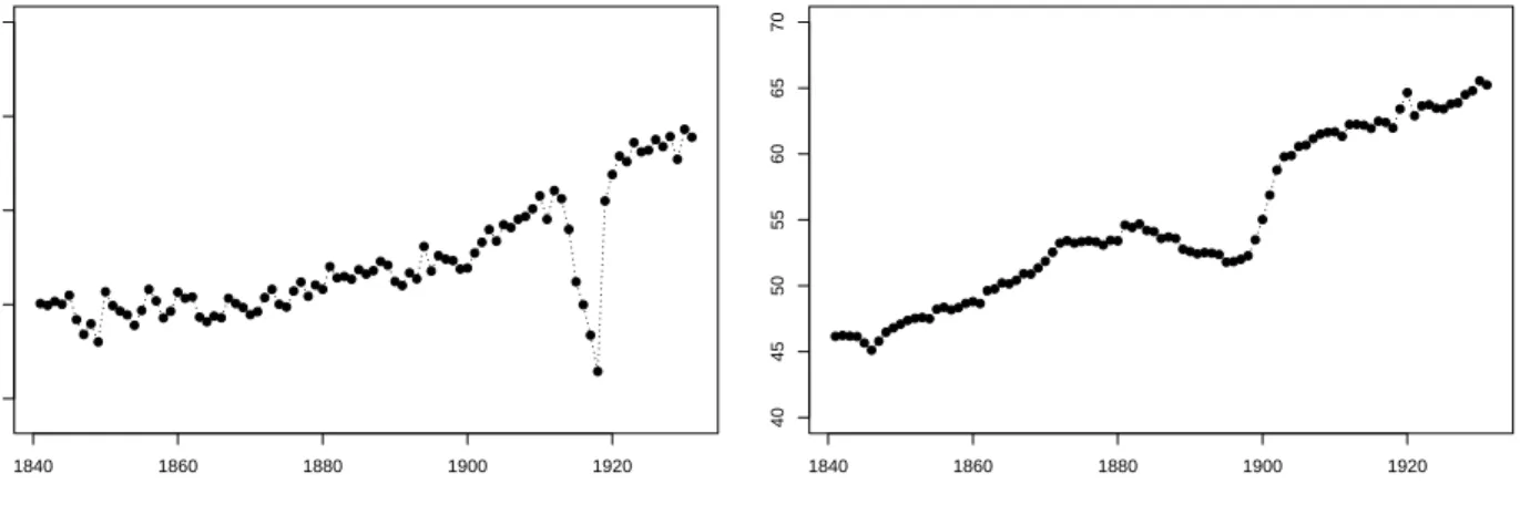
Longevity appears as a trend risk, whereas mortality is variability risk. Is there orthogonality between mortality and longevity? - In other words, can we ”buy” mortality risk in order to hedge longevity risk? Oscillations around the average trend are also important: the size of the oscillations cannot be neglected, and in any case they can lead to over-reactions by insurance managers, regulators, policy-holders and governments. Obviously, even if a certain mutualisation between mortality and longevity risks exists, it is very difficult to obtain a significant risk reduction between the two, on account of their differing natures. Indeed, the replication of life annuities with death insurance contracts could never be perfect as it concerns different individuals; thus, the hedge is often inefficient due to the variability related to the death of insured individuals whose death benefits will be high. Moreover, the impacts of a pandemic or a catastrophe on mortality is considerably different from the impacts on longevity. In fact, an abnormally high death rate at a given date has a qualified influence on the longevity trend: as it was with the 1918 flu pandemic (see Figure 3.1).
What about correlations between life and market risks? Long-term horizons have financial
conse-1840 1860 1880 1900 1920 30 40 50 60 70 year
Period life expectancy in year at birth
1840 1860 1880 1900 1920 40 45 50 55 60 65 70 year
Cohort life expectancy in year at birth
Figure 3.1: Periodic life expectancy (left) and generational life expectancy (right) at birth in the UK.
quences: if longevity risk is transferred, the interest rate and counterparty risk often become predom-inant. Financial risks are grouped into the market risk module; whereas, the longevity, mortality and disability risks are grouped into the life risk module. At a higher level, market-risk and life-risk are
aggregated in the same manner thanks to a unique correlation parameter that excludes data on the proportion of longevity and mortality risk companies are exposed to. This is a major deficit of the two-level aggregation approach as described in Filipovi´c (2009).
The correlation parameter between longevity risk and disability risk, fixed at the level−25%, is rel-atively low in QIS5. Is it realistic in practice? The loss of autonomy and increased dependency that often affects elderly people, are major demographic issues. Taking France as an example, important approaches have been introduced in order to help so called ”dependent people”. The question of long-term care insurance has a strong economic dimension, with a year of dependence costing four times more than a typical year of retirement. Consequently, a worldwide public awareness campaign about the phenomenon and its consequences is being run to promote preventative action. Moreover, levels of dependence accurately reflect individual health capital. Statistics from the INSEE reveal that when an individual enters a state of dependence, their life expectancy drops by 4 years, almost entirely irrespective of age. The INSEE statistics were obtained by factoring in all states of dependency, from the chronic dependencies such as those linked to Alzheimer’s disease, to the less severe forms, that often account for several years. Thus, individual longevity is strongly correlated to dependence level. Obtaining an idea of the global correlation between the two risks at portfolio level is difficult and requires modelling similar to that presented in Bensusan and El Karoui (2010). Finally, it is impor-tant to note that the meaning and definition of ”dependence” (or ”disability”) differs from country to country and across regulatory panels, making the correlation between longevity and dependence difficult to define.
Thus, insurers have an incentive to develop an internal model, or a partial internal risk model, to better account for the characteristics and interactions of biometric and financial risks.
3.2.2. Internal risk models
The alternative to the standard formula for calculating solvency capital requirements is the use of an internal model (or one or more partial models). In such cases, the internal model should capture the risk profile of the insurer by identifying the various risks it faces. Therefore, the internal model should incorporate the identification, measurement and modelling of the insurer’s key risks. As for internal models, the Solvency II guidelines take the position that in circumstances where an insurer prefers developing its own framework to assess the incurred risks, the Value at Risk must be used to compute the required capital. The methodology considered here is highly contrastable with the one already in use in the banking industry.
The Value at Risk measure that has been recently introduced within the insurance industry, is based on yearly available data. This highlights the main difference between the banking and insurance industries. In banking, access is assured to to high frequency data that permits computation of daily risk measures; whereas, in insurance the Value at Risk is computed over the whole year, and so can assess solvency. The required capital for the yearSCRiinsuring the solvency during this given period
and is drawn from the Value-at-Risk at levelα= 0.5% is
SCRi=V aRα(Mi)−E(Mi),
whereMi is the liabilities used to compute the associated solvency capitals. 3.3. Risk margin
Finally, the required capital has to yield a return (it is not necessarily fixed, and it depends on the internal capital targets) each year, as it is sold to shareholders who expect some return on their investment. The total margin needed to satisfy the return expected by the shareholders, is called the risk margin. Another method, called the cost of capital approach, is used determine the market price
of risk, and possible transfer values when added to the best estimate of liabilities. Regulators have highlighted the effectiveness of risk mitigation such as reinsurance and derivatives to release capital, which is especially important considering the new additional solvency requirements increase the need for capital. Therefore, capital markets are an attractive means by which to transfer the longevity risk, as the traditional reinsurance approach to risk transfer has a limited capacity to fund and absorb that risk.
3.4. Impact of longevity risk on the economy
To think beyond the Solvency II framework, a risk management analysis that incorporates dynamic correlations between both insurance and financial risks should also take into account the impacts of longevity risk upon the economy. As has been noted, many entities are concerned by longevity risk, and will find it necessary to hedge the long-term risk. For example, governments are now facing a retirement challenge coupled with associated longevity risk. The article Antolin and Blommestein (2007) highlights many of the impacts caused by longevity improvements for people aged eighty or older on GDP and political decision-making at a national level. Consequently, population ageing has macroeconomic consequences; some countries are even considering it as a factor of economic slackening.
However, this issue can be mitigated; when life expectancy increases, consumption also increases. The ageing of a population does not necessarily correspond to an economic ’ageing’ and associated decline, but could, on the contrary, inspire an economy of ageing. Innovations come in many fields, including but not limited to: medicine, home automation, urban planning and transport. In many developed countries, urban redevelopment incorporates the facilitation of many access types, including free circulation for the elderly.
In 2005, the French Academy of Pharmacy published a report ”Personnes Ag´ees et M´edicaments” (see FAP (2007)) that revealed an increase in medicine consumption by both senior citizens and the whole medical economy of ageing. Indeed, with and ageing population and growing demand, medicine consumption increases at a high rate. Moreover, the innovative pharmaceutical companies are considering the development of new medicines specifically designed for the elderly.
4. Transferring longevity risk
To recap, a steady increase in life expectancy in Europe and North America has been observed since 1960s, which has and continues to represent a significant and evolving risk for both pension funds and life insurers. Various risk mitigation techniques have been advocated to better manage this risk: reinsurance and capital market solutions in particular, have received growing interest. In February 2010, with the aim of promoting and developing a transparent and liquid market for longevity risk transfer solutions: AXA, Deutsche Bank, J.P. Morgan, Legal and General, Pension Corporation, Prudential PLC, RBS and Swiss Re established the Life and Longevity Markets Association (LLMA). The LLMA is a non-profit venture supporting the development of consistent standards, methodologies and benchmarks.
4.1. Convergence between insurance and capital markets
Even if no Insurance-Linked Securitisation (ILS) of longevity-risk has so far been implemented, the development of the market for other insurance risks has been experiencing continuous growth for several years. This growth that has been mainly driven by changes in the regulatory environment and the distinct need for additional capital in the insurance industry. Today, longevity risk securitisation lies at the heart of many discussions, and is widely seen as a viable potential.
The convergence of the insurance industry with the capital markets has become increasingly impor-tant over recent years. This convergence has taken many forms, and with mixed success. In academic discourses, the first theoretical discussion presenting the idea that capital markets could be effectively used to transfer insurance risk was presented in a paper by Goshay and Sandor (1973). The authors considered the feasibility of an organised market, questioning how such a market could complement the reinsurance industry, discussing primarily catastrophic risk management. In practice, while some attempts have been made to development an insurance futures and options market; so far the results have caused some disappointment. Despite this, the ILS market has grown rapidly over the last 15 years. Many motivations exist for using ILS instruments, including: risk transfer, capital strain relief, acceleration of profits, speed of settlement, and duration. Different motivations, require different so-lutions and structures, as the variety of instruments on the ILS market illustrates.
While the non-life section of the ILS market is the most visible, famously trading the highly successful cat-bonds, the life section of the ILS market is the bigger in terms of transaction volume. Today’s situation is varied, and there are huge contrasts between the non-life and the life ILS markets; with success, failure and future developments resting with the impacts of the financial crisis. Whilst in the non-life-sector, the credit crisis has had only a limited noticeable impact, partly due to product structuring, a dedicated investor base and a disciplined market modelling and structuring practices; the life-sector has been greatly affected by the recent crisis. This is mostly due to the structuring of deals and the nature of the underlying risks: with more than half of the transactions being wrapped, or containing embedded investment risks. Therefore, principles governing the constitution and man-agement of the collateral account, as well as the assessment of the counterparty risk are central to current debates aimed at developing a sustainable and robust market.
4.2. Recent developments in the transfer of longevity risk
Coming back to longevity risk; a number of important developments have been observed over the past 3 years, including increased attention from US and UK pension and life insurance companies, and an estimated underlying public and private exposure of over 20 trillion USD. Even if a large quantity of private equity transactions have been completed, very few overt capital market transactions - mainly taking a derivative form (swaps) - have been achieved.
Despite this limited activity, using the capital markets to transfer part of the longevity-risk is com-plementary to traditional reinsurance solutions, and would thus seem to be a natural move. To date, almost all longevity capacity has been provided by the insurance and reinsurance markets. Whilst this capacity has facilitated demand to date, exposure to longevity risk for UK pension funds alone is estimated to exceed 2 trillion GBP. It is therefore clear that insufficient capacity exists in traditional markets to absorb any substantial portion of the risk, and only capital markets are a potential capacity provider.
On face value, longevity meets all the basic requirements of a successful market innovation. However, there are some important questions to consider. To create liquidity and attract investors, annuity transfers need to move from an insurance format to a capital markets format.
As a consequence, one of the main obstacles for the development of capital market solutions would appear to be the one-way exposure experienced by investors, since there are almost no natural buyers of longevity-risk. Inevitably, this could cause problems for demand. Nevertheless, provided it is priced with the right risk-premium, there is potential for longevity-risk to be formed as new asset class, which could interest hedge funds and specialised ILS investors.
Another consideration is that basis-risk could prevent a longevity market from operating successfully. Indeed, the full population mortality indices have basis risk with respect to the liabilities of individual pension funds and insurers. Age and gender are the main sources of basis risk, but also regional and socio-economic basis risk could be significant. Therefore, the use of standardised instruments based
upon a longevity index, with the aim of hedging a particular exposure, would result in leaving the pen-sion fund or life insurer with a remaining risk often challenging to understand (and hence, to manage). An important challenge lies in developing transparency and liquidity by ensuring standardisation, but without neglecting the hedging purposes of the instruments.
Recently, many different initiatives have been undertaken in the market, which aim at increasing the transparency concerning longevity-risk and contributing to the development of longevity-risk transfer mechanisms.
4.3. Various longevity indices
Among the different initiatives to improve visibility, transparency and understanding of longevity-risk, various indices have been created. A longevity-index needs to be based on national data (available and credible) to have some transparency, but must also be flexible enough to reduce the basis-risk for the original longevity-risk bearer. National statistical institutes are in a position to build up annual indices based on national data, which could incorporate projected mortality rates or life expectancies (for gender, age, socio-economic class and so on). Potentially, such a move could limit basis-risk and help insurance companies form a weighted average index pertinent to their specific exposure.
Today, the existing indices7 are:
• Credit Suisse Longevity Index, launched in December 2005, is based upon national statistics for the US population, incorporating some gender and age specific sub-indices.
• JP Morgan Index with LifeMetrics, launched in March 2007. This index covers the US, England, Wales and the Netherlands, by national population data. The methodology and future longevity modelling are fully disclosed and open, (based upon a software platform that includes the various stochastic mortality models).
• Xpect Data, launched in March 2008 by Deutsche Borse. This index initially delivered monthly data on life expectancy in Germany, but has now been extended to include the Netherlands.
4.4. q-forwards
JP Morgan has been particularly active in trying to establish a benchmark for the longevity market. Not only have they developed the LifeMetrics longevity risk platform, but have developed standardised longevity instruments called ”q-forwards”. These contracts are based upon an index that draws upon on either the death probability or survival rate as quoted in LifeMetrics. Naturally, survivor swaps are the intuitive hedging instruments for pension funds and insurers. However, the importance assigned to the starting date of the contract (owing to the survival rate being path-dependent), may reduce the fungibility of the different contracts in relation to the same cohort and time in the future. Therefore, mortality swaps are also instruments likely to be applicable. The mechanisms of a q-forward can be summarised as follows:
The mechanisms of the q-forwards can be understood simply: a pension-fund hedging its longevity-risk will expect to be paid by the counterpart of the forward if the mortality falls by more than expected. So typically, a pension fund is a q-forward seller, while an investor is a q-forward buyer.
7The Goldman Sachs Mortality Index, launched in December 2007, was based on a sample of insured over 65s in the U.S. It targeted the life settlement market, but was discontinued in December 2009, following the global financial crisis.
Counterparty A (fixed rate payer)
Counterparty B (fixed rate receiver) Notional×100×
fixed death probability
Notional×100×
realized death probability
Figure 4.1: q-forward mechanism
Notional Amount GBP 50,000,000 Trade Date 31 Dec 2006 Effective Date 31 Dec 2006 Maturity Date 31 Dec 2016 Reference Year 2015 Fixed Rate 1.2000% Fixed Amount
Payer
JPMorgan
Fixed Amount Notional Amount×Fixed Rate×100
Reference Rate LifeMetrics graduated initial death probability for 65-year-old males in the reference year for England & Wales national pop-ulation
(Bloomberg ticker: LMQMEW65 index<GO>) Floating Amount
Payer
WYZ Pension
Floating Amount Notional Amount×Reference Rate×100
Settlement Net settlement = Fixed amount - Floating amount
Figure 4.2: An example of a q-forward contract
4.5. Longevity swap transactions and basis risk
Over the last 3 years, a number of longevity swap transactions have taken place. The transactions have occurred in private; therefore, their pricing remains confidential and subject to the negotiation between the parties involved in the deal. Some swaps were contracted between a life insurance company and a reinsurer as a particular reinsurance agreement; whilst, others have involved counterparts outside the insurance industry. Most of these transactions have a long-term maturity and incorporate an important counterparty risk, which is difficult to assess given the long term commitment. As a consequence, the legal discussions around these agreements make them a particularly drawn out contract to finalise.
Longevity swaps mainly take two forms, depending on whether they are index-based or customised. Two differing longevity swaps arranged by JP Morgan in 2008 are discussed below:
A customised swap transaction. In July 2008, JP Morgan executed a customised 40 year longevity
swap with a UK life insurer for a notional amount of GBP 500 million. The life insurer agreed to pay fixed payments, and to receive floating payments, replicating the actual benefit payments made on a closed portfolio of retirement policies. The swap is before all a hedging instrument of cash flows for the life insurer, with no basis risk.
At the same time, JP Morgan entered into smaller swaps with several investors that had agreed to take the longevity risk at the end. In this type of indemnity based transaction, the investors have access to the appropriate information to enable them to assess the risk of the underlying portfolios. The back-to-back swap structure of this transaction means that JP Morgan has no residual longevity exposure. The longevity risk is transferred from the insurer to the investors, in return for a risk premium. The counterparty risk for such a swap is important given the long term maturity of the transaction, and the number of agents involved.
A standardised transaction: Lucida. In January 2008, JP Morgan executed a 10 year standardised
longevity swap with the pension insurer Lucida for a notional sum of GBP 100 million; with an underlying risk determined by the LifeMetrics index for England and Wales. This swap structure enabled a value-hedge for Lucida, who have in this case agreed to keep the basis risk. For more details on both transactions, and longevity swaps, see Barrieu and Albertini (2009).
As previously outlined, longevity-risk is highly particular. The market for longevity-risk is also very distinct, being strongly unbalanced in terms of exposures and needs. This makes the question of the pricing of risk transfer solutions markedly important. Yet, even before this, the problem of designing suitable, efficient and attractive structures for both risk bearers and risk takers is absolutely essential to tackle. This is underlined by the failure of the EIB-BNP Paribas longevity bond8 in 2005. The
recent financial crisis has also emphasised the importance of assessing counterparty-risk, and properly managing the collateral accounts which help to secure transactions. These questions are even more critical when considering longevity-risk: firstly, due to the long-term maturity of the transactions; but secondly, the social, political and ethical nature of the risks involved.
5. Modelling issues for pricing
Designing longevity-based securities brings together various modelling issues besides form the challenges of pure longevity risk modelling. An initial issue, is that the pricing of any longevity ”derivative” is not straightforward, as it is dependent upon both estimations of uncertain future mortality-trends, and other levels of uncertainty. This risk induces a mortality-risk premium that should be priced by the market. However, because of the absence of any liquid traded longevity-security, it is today impossible to rely on market data for pricing purposes. Long-term interest rates should play a key role in the valuation of such derivatives with long maturities (up to 50 years), which is likely to create new modelling challenges.
5.1. Pricing methodologies
In this section, methodologies for pricing longevity-linked securities are investigated. As the longevity market is an immature market, based on a non-financial risk, the classical methodology of risk-neutral pricing cannot be used carelessly. Indeed, the lack of liquidity in the market induces incompleteness, as it is typically the case when non-hedgeable and non-tradable claims exist. Thus, to price some financial contracts on longevity-risk, a classical arbitrage-free pricing methodology is inapplicable as it relies upon the idea of risk replication. The replication technique is only possible for markets with high liquidity and for deeply traded assets. It induces a unique price for the con-tingent claim, which is the cost of the replicating portfolio hedging away the market risk. Hence, in a complete market, the price of the contingent claim is the expected future discounted cash-flows, calculated by the unique risk-neutral probability measure. In contrast, in an incomplete market, such
as a longevity-linked securities market, there will be no universal pricing probability measure, making the choice of pricing probability measure crucial.
What will be a good pricing measure for longevity? It is expected that the historical probability
mea-sure will play a key role, due to the reliable data associated with it. Therefore, it seems natural to look for a pricing probability measure equivalent to the historical probability measure. Important factors to consider, are that a relevant pricing measure must be: robust with respect to the statistical data, but also compatible with the prices of the liquid assets quoted in the market. Therefore, a relevant probability measure should make the link between the historical vision and the market vision. Once the subsets of all such probability measures that capture the desired information is specified, a search can commence for the optimal example by maximising the likelihood or the entropic criterion.
5.1.1. Characterisation of a pricing rule
Questions concerning the pricing rule are also essential when addressing financial transactions in an incomplete market. If a risky cash flowF with a long-term maturity is considered; for example, for the EIB-BNP Paribas longevity bond mentioned in Section 4.5, the cash flow F corresponds to the sum of the discounted coupons.
Classical static pricing methods. The change from the historical measure to the pricing measure
introduces a longevity risk premium. This method is similar to those based upon actuarial arguments, where the price of a particular risky cash-flowF can be obtained as
π(F) =EP(F) +λσP(F).
The risk premium λ is a measure of the Sharpe ratio of the risky cash-flow F. Different authors have studied the impacts of different choices of probability measures on the pricing (Jewson and Brix (2005)) for the other types of financial contracts, such as weather derivatives.
As recalled before, in a highly liquid and complete market where risky derivatives can be replicated by a self-financing portfolio, the risk-neutral (universal) pricing rule is used:
π(F) =EP∗(F) =EP(F) + cov F, dP∗
dP
.
This pricing rule is linear, as the actuarial rule does not take into account the risk induced by large transactions. However, in those cases where hedging strategies cannot be constructed, the nominal amount of the transactions becomes an important risk factor. In such cases, this methodology is no longer accurate, especially when the market is highly illiquid. A seemingly more appropriate methodology to address this problem is the utility based indifference pricing methodology presented below.
Indifference pricing. In an incomplete market framework, where perfect replication is no longer
pos-sible, a more appropriate strategy involves utility maximisation. Following Hodges and Neuberger (1989), the maximum price that an agent is ready to pay is relative to their indifference towards the transaction and according to their individual preference. More precisely, given a utility functionub
and an initial wealth ofWb
0, the indifference buyer price ofF isπb(F) determined by the non-linear
relationship: EP u b (W0b+F−πb(F) =EP u b (W0b) .
This price, which theoretically depends upon initial wealth and the utility function, is not necessarily the price at which the transaction will take place. This specifies an upper bound to the price the
agent is ready to pay. Similarly, the indifference seller price is determined by the preference of the seller, and characterised by
EP u s(Ws 0 −F+π s(F) =EP u s(Ws 0) . (5.1)
It should be noted that this pricing rule is non-linear and difficult to compute, and provides a price-range rather than a single price.
Fair price for small transactions. Agents who are aware of their sensitivity to unhedgeable risk can
attempt to transact at a low price when forming a risky contract. In this case, the buyer wants to transact at the buyer’s ”fair price”: which corresponds to the zero marginal rate of substitutionpb.
∂θEP u b (W0b+θF) |θ=0=∂θEP ub(W0b−θp(F)) |θ=0 that implies pb(F) =EP u b x(W b 0)F /EP ubx(W0b) . (5.2)
The same formula holds when the random initial wealthW0bis in fact the value of the optimal portfolio
found in the classical optimisation problem when considering the scenario of an incomplete market utility functionub. In this case, the normalised random variableub
x(W0b) may be viewed as the optimal
martingale measure.
When both agents have the same utility function, they can transact at this fair price. Therefore, with an exponential utility function, the fair price for a small transaction is equivalent to the one given by the expectation under an equivalent probability measure. This methodology can be compared to the Wang transform, which is a distortion of the historical probability (see the approach of Lin and Cox (2005)). If we linearise the Wang transform an equivalent change in probability measures can be produced. The potential shortcomings of this approach are discussed in Bauer et al. (2010).
Economic point of view. When approaching the same subject form an economic point of view, the
transaction price can be said to form an equilibrium price. This occurs between either the seller and buyer, or different players in the market. It can be described as a transaction where the agents simultaneously maximise their expected utility (Pareto-optimality). Obviously a transaction only takes place where there are two agents for whomπb(F)>πs(F).
5.1.2. A dynamic point of view
The economic pricing methodologies described in the above subsection are static and correspond in this respect mainly to an insurance or accounting point of view. However, the standard financial approach to pricing is different, as it relies on the so-called, risk-neutral methodology. The main un-derlying assumption of this approach is that it is possible to replicate cash flows of a given transaction dynamically using basic traded securities in a highly liquid market. Using a non-arbitrage argument, the price of the contract is uniquely defined by the cost of the replicating strategy. Using a risk-neutral probability measure as a reference, it can also be proven that this cost is in fact the expected value of the discounted future cash flows. This approach is clearly dynamic, since the replicating strategy is dynamically constructed. Note: the replicating portfolio is not only a tool to find the price of the contract, but can also be used to dynamically hedge the risks associated with the transaction. Since the cash flows are discounted and longevity-linked securities have a long maturity, this approach raises some specific issues relating to dynamic long-term interest-rates (see subsection 5.2.1). In any case, adopting such an approach for the pricing of financial contracts based upon mortality- or longevity-risks requires the underlying longevity-risks to be dynamically modelled (see subsection 5.2.2). It is important to emphasise that a highly liquid underlying market is essential for the construction of such a repli-cating strategy. Nevertheless, as has been mentioned, the present state of the longevity market is far
from liquid, and the applicability of risk neutral methodology has been questioned in many research papers; including Bauer et al. (2010). It could be argued that to extend the fair price approach to an illiquid and dynamic setting is an appropriate action. Since a perfect hedge does not exist, we can extend (5.2) as sup EP u s(Ws 0 −F+π s(F) =EP u s(Ws 0) , (5.3)
whereπs(F) is no longer a static price, but a dynamic price strategy associated with a hedge, and the supremum in (5.3) is taken over the strategies. Thus an optimal hedge, given criteria (5.3) is derived (see Barrieu and El Karoui (2009)).
5.1.3. Design issues
Due to the absence of liquidity and maturity in the longevity market, a dynamic replicating strategy cannot be constructed; and therefore, the various risks embedded in a longevity transaction will be difficult to dynamically hedge . As a consequence, investors will consider the pricing and design of a transaction in order to select the one, which from their point of view seems the least risky. Therefore, the design of new securities is clearly an extremely important feature of the transaction; in fact, it may mean the difference between success and failure.
The problem that will be considered next, is the design of a contractF and a price π(F) that are desirable for both the buyer and seller to form a transaction. Such a problem is studied in detail by Barrieu and El Karoui (2009). An interesting feature of the risk transfer emerges when both agents have the same utility function but different risk tolerances: ub(x) =γbu(x/γb) andus(x) =γsu(x/γs). Given an initial risk that the seller wants to partially transfer to the buyer, the best choice is to transfer F∗ = γsγ+bγbX. Thanks to the optimality ofF
∗, it can be shown that a pricing probability
measure common to both agents still exists, but that it depends upon the pay-out of the derivatives. Nevertheless, this feature is in some ways simplistic, as investors do not usually share the same utility function (because, for example, they do not have access at the same market). Thus, such issues are not reduced in the transfer mentioned above; but, in fact, become more crucial and complex.
5.2. Dynamic modelling of the underlying risk
Dynamic pricing approaches raise a number of issues related to the modelling of the underlying risk. In addition to longevity-risk, financial contracts on longevity are also exposed to long-term interest rate risk. Due to the lack of liquidity on the long-term horizon, the interest rate risk should be handled differently from the rate explored in typical financial modelling. In addition, as introduced in Section 2, the underlying longevity-risk should be undertaken through a continuous-time rather than a discrete-time framework.
5.2.1. Long-term interest rates
Financial contracts on mortality-related risks, typically have a maturity up to 20 years. Whilst in contrast, longevity-linked securities are typically characterised by a much longer maturity (40 years and beyond). In the case of the vast majority of such contracts, there is an embedded interest rate risk. For the shorter-term time-horizon, the standard financial models perform appropriately to model the underlying risk. However, this is no longer the case for longer maturities. In such scenarios, the interest rate market becomes highly illiquid and the typical financial attitude is not easily extendable. Nevertheless, an abundant literature on the economic aspects of long-term policy-making has been developed (see for example Gollier (2007, 2008), Hansen and Scheinkman (2009) or Breeden (1979)). Much of this discourse focuses on the aggregate behaviour of all agents, and the representation of the economy is limited to the strategy of the representative agent. The derivation of the yield-curve for far-distant maturities is induced from the maximisation of the representative agent’s inter-temporal utility