Parallel Space Decomposition of the Mesh
Adaptive Direct Search algorithm
∗
Charles Audet
†J.E. Dennis Jr.
‡S´ebastien Le Digabel
§April 11, 2008
Abstract
This paper describes a Parallel Space Decomposition (PSD) technique for the
Mesh Adaptive Direct Search (MADS) algorithm. MADSextends Generalized Pat-tern Search for constrained nonsmooth optimization problems. The objective of the present work is to obtain good solutions to larger problems than the ones typi-cally solved by MADS. The new method (PSD-MADS) is an asynchronous parallel algorithm in which the processes solve problems over subsets of variables. The convergence analysis based on the Clarke calculus is essentially the same as for the MADSalgorithm. A practical implementation is described and some numerical results on problems with up to 500 variables illustrate advantages and limitations of PSD-MADS.
Keywords: Parallel Space Decomposition, Mesh Adaptive Direct Search (MADS),
Asynchronous parallel algorithm, Nonsmooth optimization, Convergence analysis.
∗Work of the first author was supported by FCARgrant NC72792 and NSERCgrant 239436-05. The second author was supported by LANL94895-001-04 34. Both were supported by AFOSR FA9550-07-1-0302, the Boeing Company, ExxonMobil Upstream Research Company, and the first and third authors were supported by the Consortium for Research and Innovation in Aerospace in Qu´ebec (CRIAQ).
†GERADand D´epartement de math´ematiques et de g´enie industriel, ´Ecole Polytechnique de Montr´eal, C.P. 6079, Succ. Centre-ville, Montr´eal (Qu´ebec), H3C 3A7 Canada,www.gerad.ca/Charles.Audet, [email protected]
‡Computational and Applied Mathematics Department, Rice University, 8419 42nd Ave SW, Seattle, WA98136http://www.caam.rice.edu/∼dennis,[email protected]
§GERADand D´epartement de math´ematiques et de g´enie industriel, Ecole Polytechnique de Montr´eal, [email protected]
1
Introduction
This paper considers optimization problems of the form
min
x∈Ωf(x) (P)
with the objective function f : Ω ⊂ Rn →
R∪ {∞}. Our motivation is to treat P whenngrows large. The feasible regionΩis assumed to satisfy a nonsmooth constraint qualification, which we will discuss later, and we only assume the presence of an oracle to tell whether or not a given x ∈ Rn is feasible. We are concerned primarily with cases wheref(x)or the oracle are given by black-box computer simulations, which are assumed to evaluate in finite time. This is common in engineering design. Indeed, the reason we allowf(x)to take on the value∞is that for many such problems, no value of
f(x)is returned even forx∈Ωbecause of the internal workings of the simulation used to drive the design. See [1,3,10,13,21,27,32,42].
There are other useful derivative-free direct search methods designed for problems similar toP. These include the Nelder-Mead simplex [43], the DIRECTalgorithm [20,
24, 30], the frame based methods [16, 44], the Generalized Pattern Search (GPS) [7,
14, 49], the Asynchronous Parallel Pattern Search (APPS) approach [25, 29, 33, 35,
36], and the Mesh Adaptive Direct Search (MADS) [2, 8]. Related is the implicit filter method [31], though it does use a coarse difference gradient approximation. The reader may consult [31,34,39] for a survey of some of these direct search methods.
Using these methods to solve expensive problems with more than a few dozen vari-ables may be impractical since they may need a large number of costly black-box eval-uations. Dennis and Wu [18] reviewed different parallel methods for continuous opti-mization and concluded that a combination of GPSand the Parallel Variable Distribution (PVD) of Ferris and Mangasarian [19] should be considered:
“. . . parallel variable distribution and parallel direct searches seem an inter-esting pairing. . . ”.
The present paper is based on this remark.
PVDis an evolution of the block-Jacobi technique of [11] which optimizes in parallel a series of reduced subproblems on subspaces of the original variables of P. Dennis and Torczon [17] described a first parallel version of GPS, which evaluates the black-box in parallel and synchronizes at each iteration to compare solutions and update the current iterates. The Asynchronous Parallel Pattern Search, APPS[25,33], removes this synchronization barrier. In APPS, each process explores the space of variables using its own set of directions and does not wait for the other processes to terminate. APPS is expected to be more efficient than the synchronous version of [17], especially if the black-box has heterogeneous behavior that depends on the point where it is evaluated. A convergence analysis is presented in [36] for the smooth case.
Our work applies a decomposition of the variables ofP based on the block-Jacobi technique of [11] that inspired the PVDmethod of [19]. This allows a natural parallel ap-plication of MADSto smaller subproblems, in an asynchronous way. The new algorithm, called PSD-MADS, can be interpreted as a particular instance of MADS, thus inheriting the main results of the MADSconvergence analysis. The paper focuses on the definition of the PSD-MADS frameworks and on its convergence analysis, and not on the choice of the subproblem variables. In our practical implementation of the algorithm, a simple random strategy is used, and it performs well.
The paper is divided as follows: Section 2gives an overview of the Parallel Space Decomposition and MADS methods. Section 3 presents the new asynchronous paral-lel algorithm, PSD-MADS, and Section 4ensures that the main convergence results of MADS are maintained by showing that the entire PSD-MADS algorithm may be inter-preted as a specific MADS instance. An implementation of PSD-MADS is described in Section5, with some numerical results on problems with a number of variables rang-ing from 20 to 500. Finally, Section6 gives some conclusions and proposes possible extensions of PSD-MADS.
2
Relevant literature
This section presents an overview of parallel space decomposition methods. The Mesh Adaptive Direct Search algorithm, its convergence analysis and its LTMADS implemen-tation are also described in detail.
2.1
Parallel space decomposition methods
Parallel space decomposition methods decompose P into a finite number of smaller dimension subproblems, which can be solved in parallel with one process assigned to each subproblem.
Define N = {1,2, ..., n} where n is the number of variables of the optimization problemP, and Q = {1,2, ..., q} whereq is the number of available processes. Each processp∈Qworks on a nonempty subsetNp ⊆Nof the variables. The other variables are fixed, based on the incumbent solution x∗ ∈ Ω, the current best known solution. More precisely, processp∈Qworks on the optimization subproblem
min
x∈Ωp(x∗)
f(x) (Pp(x∗))
withΩp(x∗) =
x∈Ω :xi =x∗i ∀i∈Np andNp =N\Np. The subproblemPp(x∗)
containsnp =|Np|free variables, indexed byNp. In Section5we propose a simple and random strategy to build the subsetsNp.
The block-Jacobi method in [11] is an iterative two-step algorithm and may be de-scribed in a very general way as follows. At each iteration, the first step, the paral-lelization, consists in solving the subproblems in parallel, and the second step, the syn-chronization, gathers the subproblem solutions and constructs the next iterate. Similar methods are described in [26,41,50].
A variant of the method was introduced by Ferris and Mangasarian [19], as the Paral-lel Variable Distribution (PVD) for a differentiable objective functionf with continuous partial derivatives. In order to solve the subproblems more efficiently, the PVDmethod allows a priori fixed variables to change in a limited fashion, along directions typically based on∇f. These variables are denoted as “forget-me-not” terms.
The convergence analysis in [19] requires that subproblems be solved to optimality. In the unconstrained case, if∇f exists and is Lipschitz, then the accumulation points of the generated sequences are stationary points. In addition, iff is assumed to be convex, the convergence rate is shown to be linear. WhenΩis nonempty, closed, convex, block-separable, and the functions defining it are also continuously differentiable, convergence results are still available. When there are general constraints, Ferris and Mangasarian recommend transforming the problem into unconstrained problems via penalty func-tions. This strategy is untested as far as we know, and we prefer to avoid estimating penalty constants.
These are parallel synchronous algorithms because the synchronization step waits for all the processes to end. The conclusion of [19] states that an asynchronous version of the algorithm would increase efficiency. This is done in [40] for unconstrained problems, where the synchronization step is dropped at the expense of the convergence analysis.
Extensions of the PVD method are given in [45, 46, 47] with similar convergence results to those in [19] under less restrictive conditions. For example, subproblems do not need to be solved to complete optimality, as for example when one Newton-like iteration is used. A convergence analysis for the constrained case is given with either block-separability or convexity assumptions on the structure ofΩ.
In the above references, no practical and generic strategy is given concerning the choice of the subproblem variables (sets Np). However, the sets do need to form a partition ofN, and they are fixed throughout the entire process. In the parallel space decomposition [22] the subspaces can be chosen differently at each iteration.
Fukushima [23] extends the PVD method to a more general framework for uncon-strained problems. The sets of subproblem variables are not fixed through the iterations, are not required to form a partition ofN, but they must spanN. In particular, an over-lapping of the subproblem variables is allowed. Some experiments with such methods are given in [51].
More recently, the MOVARSalgorithm [12] combines the GPSmethod with the syn-chronous PVDframework (including the “forget-me-not” terms from [19]) on fixed sub-setsNp, but there is no convergence analysis.
and constraints, if they are considered, are block-separable or convex. These are not rea-sonable assumptions for our target class of engineering design problems, and thus, our convergence analysis does not rely on the analysis of [19] or its extensions. Rather, by incorporating MADSwith its weaker hypotheses, we will inherit the MADSconvergence analysis. It will also give us greater flexibility concerning the way to handle constraints, the amount of work devoted to the subproblems, the lack of necessity for a synchroniza-tion step, and for the choice of the subsetsNp. Concerning this last issue, we remind the reader that we will not propose an elaborated strategy for this, as the focus of the paper is first to define the new method.
2.2
Mesh Adaptive Direct Search (M
ADS)
We now summarize the MADS algorithm [8] for problemP, which extends the Gener-alized Pattern Search (GPS) algorithm for linearly constrained optimization [14,49].
The constraints definingΩare handled by the extreme barrier approach, as in [8,37,
38]. This means that trial points outside Ωare simply rejected by setting their objective function value to +∞. Of course, this requires that the user provide a feasible initial pointx0 ∈Ω. We make the standard assumption that all the trial points generated by the
algorithm lie in a compact set.
MADS is an iterative algorithm where the black-box functions are evaluated at some trial points that are either accepted as new iterates because they are feasible and decrease the objective, or rejected.
All trial points generated by these algorithms are constructed to lie on a mesh
M(∆) =
x+ ∆Dz : x∈V, z ∈NnD ⊂
Rn (1)
where the setV, called the cache, is a data structure memorizing all previously evaluated points so that no double evaluations occur, ∆ ∈ R+ represents a mesh size parameter,
andDis a n×nD matrix representing a fixed finite set of nD directions inRn. More precisely,Dis called the set of mesh directions and is chosen so thatD=GZ, whereG
is a non-singularn×nmatrix, andZan×nDinteger matrix. The definition given by (1) differs slightly from the one in [8]. There the mesh was indexed by the iteration number instead of being parameterized by∆. The reason for this difference is that our parallel algorithm will be working simultaneously on different size meshes originally generated at different iterations. Note also that in order to simplify the notation, the mesh size parameter∆used here is the equivalent of∆min [8].
Each iteration is divided into three steps, the search, the poll, and an update step determining the success of the iteration and producing the next iterate. The search and poll are treated specially in that the poll needs not be carried out at an iteration if the search finds a better point. At each iteration, the algorithm attempts to generate an improved incumbent solution on the current meshM(∆k), where ∆k is the mesh size parameter at iteration k. The search step is very flexible and allows for trial points
anywhere on the mesh. The way of generating these points is free of any rules, as long as they remain on the current meshM(∆k)and that the search terminates in finite time. Some search strategies can be tailored for a specific application, while others are generic, such as the use of Latin Hypercube sampling [48], or Variable Neighborhood Search [4]. In summary, if one wants to define a MADSalgorithm with a specific search, all that needs to be done to ensure convergence is to show that the search requires finite time and generates a finite number of trial points lying on the mesh.
The poll step explores the meshM(∆k)near the current iteratexkand its rules ensure theoretical convergence of the algorithm. The way of choosing the directions used to generate the poll points is the difference between GPS and MADS. In GPS, the set of normalized potential poll directions must be chosen from a finite set that is fixed across all iterations. In MADS, the normalized directions may be chosen to be asymptotically dense in the unit sphere, which allows better coverage. We use the terminology of [16,
44] and say that at iterationk, the set of trial poll points is called the framePk. The set of directions used to constructPkis denotedDk, and it is not a subset ofD.
In the last step of thekth iteration, the mesh size parameter is updated according to
∆k+1 ←τωk∆k, whereτ >1is a fixed rational number andωkan integer that depends on the success of the iteration. When no improvement is made, the iteration is said to fail, andωk is taken to be an integer in the interval[ω−;−1]withω− ≤ −1, forcing the next trial poll points to be closer to the current iterate. When a new best iterate is found, the iteration is said to succeed, and∆k is possibly increased withωkin[0;ω+], with the integerω+ ≥0. Specific values forτ,ω−, andω+, are suggested in Section2.4.
A high level description of the algorithm is summarized in Figure1. We encourage the reader to consult [8] for a complete description.
2.3
M
ADSconvergence analysis
We will summarize the main convergence results for MADS given in [8]. These results assume that constraints are treated by the extreme barrier approach, and they constitute a hierarchical series of results relying on the Clarke calculus [15] for nonsmooth functions. The main theorem is that under a local Lipschitz assumption on f, and under the assumption that the set of all normalized poll directions is dense in the unit sphere, the algorithm produces a Clarke stationary point. More precisely, MADS generates a point
ˆ
x ∈ Ωat which the Clarke generalized directional derivatives off in all the directions in the Clarke tangent cone atxˆare non negative. The only assumptions needed are that
f is Lipschitz nearxˆand the constraint qualification that the hypertangent cone ofΩat
ˆ
xis nonempty. A corollary to this result in the unconstrained case is that iff is strictly differentiable nearxˆ, then∇f(ˆx) = 0.
The convergence result that requires the least assumptions on f andΩ, the zero’th order result, is that MADS generates a limit point xˆ, which is the limit of mesh local minimizers on meshes that get infinitely fine. The notion of local optimality is with
M
ADS[0] I
NITIALIZATIONS x0∈Ω,∆0 >0,k←0[1] P
OLL AND SEARCH STEPSobjective: find ay ∈M(∆k)∩Ωsuch thatf(y)< f(xk) SEARCH STEP(optional)
evaluate the functions on a finite number ofM(∆k)points POLL STEP(optional if the search step succeeded)
generatendirMADSdirectionsdi∈Rn evaluate the functions on the MADSframe
Pk ={xk+ ∆kdi:i= 1,2, . . . , ndir} ⊆M(∆k)
[2] U
PDATESxk+1←y(iteration success)ORxk(iteration failure) ∆k+1←τωk∆k(reduced if iteration fails)
k←k+ 1
GOTO[1]IFno stopping condition is verified
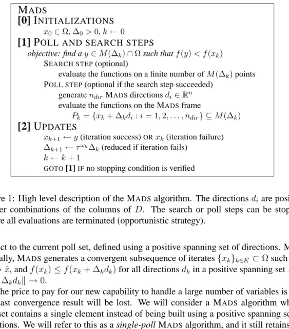
Figure 1: High level description of the MADSalgorithm. The directionsdi are positive integer combinations of the columns of D. The search or poll steps can be stopped before all evaluations are terminated (opportunistic strategy).
respect to the current poll set, defined using a positive spanning set of directions. More formally, MADS generates a convergent subsequence of iterates{xk}k∈K ⊂Ωsuch that
xk→xˆ, andf(xk)≤f(xk+ ∆kdk)for all directionsdkin a positive spanning setDK, andk∆kdkk →0.
The price to pay for our new capability to handle a large number of variables is that this last convergence result will be lost. We will consider a MADS algorithm whose poll set contains a single element instead of being built using a positive spanning set of directions. We will refer to this as a single-poll MADS algorithm, and it still retains the property of generating asymptotically dense polling directions.
The next section discusses the LTMADS (Lower-Triangular MADS) implementation of the MADS algorithm. LTMADS uses positive bases to construct the poll sets. It is stated that the union of theses normalized directions forms a dense set because if one looks closely at the proof in [8], one sees that it is the subset of single-poll normalized MADSdirections that grows dense in the unit sphere. Thus, with the assumption of local Lipschitz continuity the main convergence result guaranteeing a Clarke stationary point holds.
2.4
The L
TM
ADSimplementation of M
ADSMADS is a general class of algorithms, where the search and poll steps need to sat-isfy certain conditions for the convergence results to hold. In particular, one of these conditions is that the total set of normalized poll directions used by the algorithm is dense in the unit sphere. In [8], after the definition of the MADS framework, a practi-cal implementation is given. This implementation is named LTMADS since it implies the random construction of a lower triangular matrix. At this moment, LTMADS is the only published MADS implementation, and all MADS codes in Section 5.2 correspond to LTMADS.
LTMADS fixes τ to 4, ω− = −1, ω+ = 1, and the set of mesh directions D = [−In In] where In represents the n × n identity matrix. The mesh is based on the nonnegative integer value ` = −log4(∆k), ∆k = 4−`, and directions are constructed randomly using a lower triangular matrix. One of these directions is a special case and fixed just once for each value of`. This direction, calledb(`), has one coordinate set to
±2` so that poll points are within√∆
kof the poll centerxkin the`∞norm.
The result stated in [6,8] is that with probability one, the series of normalized direc-tionsb(`)grows dense in the unit sphere. In LTMADS, the directionb(`)is augmented at each iteration with other directions to form a positive spanning set of polling directions. We can, as explained in the preceding section, construct a single-poll MADS algorithm with dense polling directions using only theb(`)directions, but the zero’th order con-vergence result of MADS is lost. Also, because we are not polling at each iteration in a positive spanning set of directions, the mesh size might drop too quickly with this single-poll version of MADS, and so the search step is of extra importance. This is the key to the PSD-MADS algorithm described in the next section: one process executes a single-poll MADS algorithm, while the work of the other processes may be interpreted as a search step.
3
Parallel Space Decomposition of M
ADS
(P
SD
-M
ADS
)
This section describes the combination of MADS with a parallel space decomposition method. The resulting algorithm is called PSD-MADS. It is an asynchronous parallel algorithm where a master process decides on the subsetsNp ⊆ N and assigns the re-sulting optimization subproblemsPp(x∗)to slaves. The slaves apply MADS to attempt
to improve the incumbent solutionx∗. No synchronization step is performed. When a slave completes its assigned task, the master assigns a new subproblem with a possible newNpandx∗.
3.1
General description of P
SD-M
ADSAlthough PSD-MADS is an asynchronous parallel algorithm, the notion of iteration is kept, and it corresponds to two successive calls by the master to one special slave, called the pollster slave, described more precisely in Section3.2. The pollster slave executes a single-poll MADS algorithm on the entire problemP, while the other slaves, called the regular slaves, work on the subproblemsPp(x∗). This task partition between the pollster
and the regular slaves allows the convergence analysis of Section4, where it is shown that the pollster slave executes a valid MADSalgorithm, thus inheriting the convergence results of [8]. Note that the pollster slave’s task requires the fewest function values of any of the poll steps.
Each subproblemPp(x∗)is a subproblem of P with a reduced number of variables
indexed by the setNp. When an optimization process terminates, the slave communi-cates its progress to the master. If it has found an improved solution, then that becomes the new incumbent solution. The slave immediately starts work on a new subproblem assigned by the master. There is no need to synchronize all the slaves.
With several MADSinstances executing in parallel, it is necessary to define different mesh size parameters. First,∆pjcorresponds to the meshM(∆pj)used at iterationjof the MADS algorithm performed by a regular slavesp. The mesh size parameter is denoted differently for the pollster slave, with∆1k(notice the same iteration counterkused both for the pollster slave and PSD-MADS). The number∆1
k is called the pollster mesh size parameter at iterationkof PSD-MADS. Finally, an additional mesh size parameter,∆M
k , is called the master mesh size parameter. The meshM(∆Mk )is never used explicitly, but it is useful to compare the two other meshes. At iterationk of PSD-MADS, and at iterationj of the MADSalgorithm performed on a subproblemPp(x∗)by a regular slave
spforp∈Qreg, the PSD-MADS construction ensures that
∆1k ≤∆Mk ≤∆pj . (2)
Inequalities (2) are formally proved in the convergence analysis of Section 4, where PSD-MADSis interpreted as a valid single-poll MADSinstance performed by the pollster slave. An additional hypothesis on the different meshesM(∆M
k ), M(∆1k), andM(∆ p j) is necessary:
Hypothesis 3.1 If two mesh size parameters∆and∆0 satisfy∆ =τω∆0 whereω ∈
N, thenM(∆)⊆M(∆0).
This assumption holds for the PSD-MADS implementation given in Section5.
Theqprocesses are partitioned into a master,q−2slaves, and a cache server (process numberq−1), which memorizes all points that have been evaluated. Theq−2slaves include the pollster slave (process number1) andq−3regular slaves. The notation sp withp ∈ Q\ {q−1, q}is used to identify theq−2processes assigned as slaves, and
process is used as the master, which defines the lower dimensional subproblemsPp(x∗)
and communicates them to the slaves.
An advantage of applying the parallel space decomposition method to MADSinstead of another optimization method is that most of the conditions necessary for convergence in other parallel space decomposition methods mentioned in Section2.1can be relaxed (smoothness of the functions, conditions on the constraints, no synchronization step, and no restrictions on the choice of the setsNp).
This new algorithm is not a particular case of the method in [23], which generalizes many parallel variable decomposition methods, since general constraints are allowed, andf is not assumed to be smooth. PSD-MADS also differs from the recent MOVARS algorithm [12], which does require Np to partition the variables, because it provides a convergence analysis, dynamically changes the sets Np, and it is an asynchronous parallel method. The next sections describe precisely the role of each process.
3.2
The pollster slave
s
1, on
M
(∆
1k)
The pollster slaves1has a special role; its set of variables is always fixed toN1 =N, so
that it works on the original problemP. Due to its greater impact on the algorithm and to distinguishs1from the other slaves, we call it the pollster slave, or simply the pollster.
To reduce the expected high number of evaluations done by all the pollster instances, a single-poll MADS algorithm is used (the poll directions are reduced to a single ele-ment), with the conditions that the union of all the normalized directions used through-out the algorithm are dense in the unit sphere, and that the norms of those directions is in the proper relation with the mesh size parameter.
Moreover, the pollster is limited to only one MADSiteration, with no search step and one poll step. It follows that at most one function evaluation will be performed (zero function evaluation if the unique poll trial point is found in the cache), and the pollster mesh size parameter∆1kwill not be updated (this is done by the master).
The notation MADS(pollster) or MADS(s1) refers to the single-poll MADSalgorithm
performed by the pollster. MADS(pollster) is defined so that its mesh size parameter∆1
k cannot be larger than the master mesh size∆Mk at iterationkof PSD-MADS.
The pollster pseudocode is shown in Figure2. The pollster mesh size is updated by the master. The best obtained solution corresponds to xp, which is sent to the master. The convergence analysis in Section 4 is based on the pollster, and on the fact that consecutive runs of MADS(s1) form a valid single-poll MADSinstance onP.
3.3
The regular slaves
s
2to
s
q−2, on
M
(∆
pj)
The regular slavessp, p ∈ Qreg, work on subsets Np ofN, and use positive spanning sets of directions. The MADS algorithm working on problemPp(x∗)and performed by
P
OLLSTER(p= 1)Inputs : pollster mesh size∆1k
starting pointx0
Output : pollster solutionxp solve problemP: MADS(pollster) terminate after a single evaluation sendxp to master
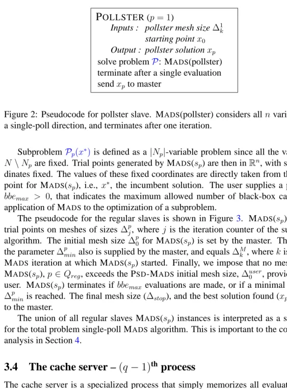
Figure 2: Pseudocode for pollster slave. MADS(pollster) considers alln variables with a single-poll direction, and terminates after one iteration.
SubproblemPp(x∗)is defined as a|Np|-variable problem since all the variables in
N \Np are fixed. Trial points generated by MADS(sp) are then inRn, with some coor-dinates fixed. The values of these fixed coorcoor-dinates are directly taken from the starting point for MADS(sp), i.e., x∗, the incumbent solution. The user supplies a parameter,
bbemax > 0, that indicates the maximum allowed number of black-box calls for the application of MADS to the optimization of a subproblem.
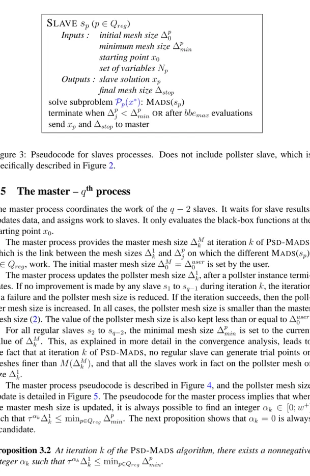
The pseudocode for the regular slaves is shown in Figure 3. MADS(sp) generates trial points on meshes of sizes∆pj, where j is the iteration counter of the subproblem algorithm. The initial mesh size ∆p0 for MADS(sp) is set by the master. The value of the parameter∆pmin also is supplied by the master, and equals∆Mk , wherek is the PSD-MADS iteration at which MADS(sp) started. Finally, we impose that no mesh size for MADS(sp), p∈ Qreg, exceeds the PSD-MADSinitial mesh size,∆user0 , provided by the
user. MADS(sp) terminates if bbemax evaluations are made, or if a minimal mesh size
∆pmin is reached. The final mesh size (∆stop), and the best solution found (xp), are sent to the master.
The union of all regular slaves MADS(sp) instances is interpreted as a search step for the total problem single-poll MADS algorithm. This is important to the convergence analysis in Section4.
3.4
The cache server –
(
q
−
1)
thprocess
The cache server is a specialized process that simply memorizes all evaluated points. Each time a process generates a trial point the cache server is interrogated. This is done to avoid unnecessary expensive functions evaluations in case this point has already been evaluated. The cache server allows the global availability of any improvement made by any slave. This is interpreted in Section 5 as a search step (the cache search) by the regular slaves on their subproblems.
S
LAVEs
p(p∈Qreg)Inputs : initial mesh size∆p0
minimum mesh size∆pmin
starting pointx0
set of variablesNp Outputs : slave solutionxp
final mesh size∆stop solve subproblemPp(x∗): MADS(sp)
terminate when∆pj <∆pmin ORafterbbemax evaluations sendxp and∆stopto master
Figure 3: Pseudocode for slaves processes. Does not include pollster slave, which is specifically described in Figure2.
3.5
The master –
q
thprocess
The master process coordinates the work of theq−2slaves. It waits for slave results, updates data, and assigns work to slaves. It only evaluates the black-box functions at the starting pointx0.
The master process provides the master mesh size∆Mk at iterationkof PSD-MADS, which is the link between the mesh sizes∆1
kand∆ p
j on which the different MADS(sp),
p∈Qreg, work. The initial master mesh size∆M0 = ∆user0 is set by the user.
The master process updates the pollster mesh size∆1k, after a pollster instance termi-nates. If no improvement is made by any slaves1tosq−1during iterationk, the iteration
is a failure and the pollster mesh size is reduced. If the iteration succeeds, then the poll-ster mesh size is increased. In all cases, the pollpoll-ster mesh size is smaller than the mapoll-ster mesh size (2). The value of the pollster mesh size is also kept less than or equal to∆user
0 .
For all regular slaves s2 to sq−2, the minimal mesh size ∆pmin is set to the current value of∆Mk . This, as explained in more detail in the convergence analysis, leads to the fact that at iterationk of PSD-MADS, no regular slave can generate trial points on meshes finer thanM(∆M
k ), and that all the slaves work in fact on the pollster mesh of size∆1k.
The master process pseudocode is described in Figure4, and the pollster mesh size update is detailed in Figure5. The pseudocode for the master process implies that when the master mesh size is updated, it is always possible to find an integer αk ∈ [0;w+] such thatταk∆1
k ≤ minp∈Qreg∆ p
min. The next proposition shows thatαk = 0is always a candidate.
Proposition 3.2 At iterationkof the PSD-MADS algorithm, there exists a nonnegative integerαksuch thatταk∆1k≤minp∈Qreg ∆
p min.
M
ASTER[0]
INITIALIZATIONSx∗ ←x0 ∈Ω,∆10 ←∆M0 ←∆user0 >0,k ←0
start MADS(pollster) with (∆user0 ,x0) (Figure2)
FOR ALL(p∈Qreg)
constructNp and set∆pmin ←∆M0
start MADS(sp) with (∆user0 ,∆
p
min,x0,Np) (Figure3)
[1]
ITERATIONSgiven values from a slavesp (∆stop,xp) IF f(xp)< f(x∗)
(success)
x∗ ←xp
IF(p= 1) pollster,∆stop corresponds to∆1k
∆M k+1 ←ταk∆1k ≤ min p∈Qreg ∆pmin withαk∈[0;ω+],ω+ ∈N ∆1k+1 ←τωk∆1 k(Figure5) k←k+ 1
start MADS(pollster) with (∆1
k,x
∗) (Figure2)
ELSE(regular slave) constructNp
∆pmin ←∆M k
∆p0 ←τγ∆stopwithγ ∈Zand so that∆Mk ≤∆ p
0 ≤∆user0
start MADS(sp) with (∆p0,∆
p min,x
∗
,Np) (Figure3) GOTO[1]IFno stopping condition is verified
Figure 4: Pseudocode for master process. ∆M
k and∆1k are the master and pollster mesh sizes at iterationk, and∆stopthe last mesh size of a slave sp. Ifp = 1, ∆stop = ∆1k ≤
∆M
k , and else∆stop≥∆Mk . The master evaluates the black-box just once forx0.
POLLSTER MESH SIZE UPDATE∆1k+1 ←τωk∆1 k IF(iteration success)
ωk =αk ∈[0;ω+],ω+≥0 ∆1k+1 ←∆Mk+1
pollster mesh size increase,∆1
k+1 ≥∆1k
ELSE
ωk ∈[ω−;−1],ω− ≤ −1
pollster mesh size decrease,∆1
k+1 <∆1k
Figure 5: Update of the next pollster mesh size∆1k+1. In any case, the pollster mesh size verifies∆1
Proof. At iteration 0,∆10 = ∆M0 = ∆user0 = minp∈Qreg∆ p
minsoα0 = 0, and therefore it
exists. Then∆M
1 = ∆user0 andminp∈Qreg∆ p
min at iteration1is equal to∆user0 . Figure5
ensures that∆1
1is bounded above by∆user0 , and thereforeα1 = 0is a possible value.
Suppose, by way of induction, that for somek ≥2, the proposition is true at iteration
k −1. It follows that ∆M
k = ταk−1∆k1−1 ≤ minp∈Qreg, and as it corresponds to new values for∆pmin,p∈Qreg, the new smaller possible value ofminp∈Qreg∆
p
minat iteration
k remains∆Mk . The largest value that ∆k1 may take is also∆Mk , which shows αk = 0 validates the result.
This proof allows all values of αk to be zero, but in practice, non-zero values are likely. For example, if iteration 1 failed and ∆11 = ∆user0 , then the following mesh updates are possible: ∆M2 ← ∆user0 (α1 = 0) and∆12 ← ∆user0 /4. minp∈Qreg∆
p min is still equal to∆user
0 at iteration2, and soα2 can be either0or1.
4
Convergence analysis of P
SD
-M
ADS
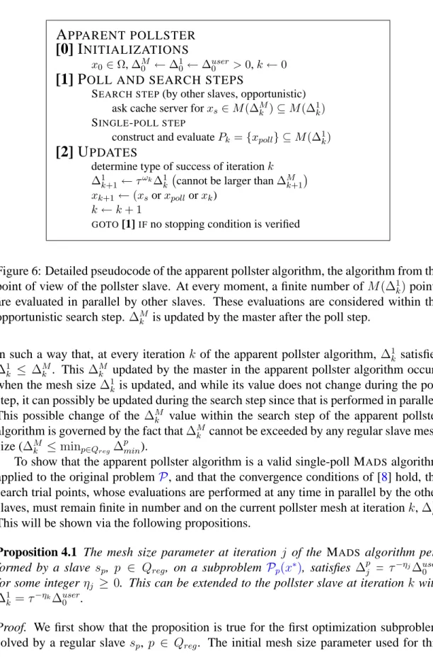
It is shown here that the entire algorithm may be interpreted as a single-poll MADS algorithm applied to the original problemP and that conditions are met so that the main convergence results from [8] hold. These conditions are that the regular slaves generate a finite number of trial points lying on the the pollster mesh, and that all these trial points can be interpreted as a search step with the pollster slave providing the poll step. This is detailed in Figure6, and we refer to it as the apparent pollster algorithm. This algorithm is another way of interpreting the PSD-MADS algorithm described by the pseudocodes in Figures 2, 3, 4, and 5. Iteration k of the apparent pollster algorithm corresponds to the iterationk of PSD-MADS (used by the master process), and the notions of iteration success and failure remain the same.
The convergence analysis in this section proves that the apparent pollster algorithm is a single-poll MADSalgorithm with the following components:
• A search step performed by regular slaves s2, s3, ..., sq−2 on mesh coarseness
larger than or equal to∆M k ;
• A poll step at iteration k (the same k used by the master process in Figure 4) performed by one call to the pollster slaves1on a mesh of size∆1k ≤∆Mk ;
• A mesh update performed by the master process with ∆1k+1 ← τωk∆1
k and the integerωk ∈
[0;ω+] iteration success
[ω−;−1] iteration failure.
The master mesh size parameter ∆Mk at iteration k is the link described by in-equalities (2) between the mesh size of MADS(pollster) and the different mesh sizes of MADS(sp). It is updated by the master with the MADS(pollster) mesh (via∆stop = ∆1k),
A
PPARENT POLLSTER[0] I
NITIALIZATIONSx0 ∈Ω,∆M0 ←∆01 ←∆user0 >0,k←0
[1] P
OLL AND SEARCH STEPSSEARCH STEP(by other slaves, opportunistic) ask cache server forxs∈M(∆Mk )⊆M(∆1k) SINGLE-POLL STEP
construct and evaluatePk={xpoll} ⊆M(∆1k)
[2] U
PDATESdetermine type of success of iterationk ∆1k+1 ←τωk∆1
k cannot be larger than∆Mk+1
xk+1 ←(xsorxpollorxk) k←k+ 1
GOTO[1]IFno stopping condition is verified
Figure 6: Detailed pseudocode of the apparent pollster algorithm, the algorithm from the point of view of the pollster slave. At every moment, a finite number ofM(∆1
k)points are evaluated in parallel by other slaves. These evaluations are considered within the opportunistic search step.∆M
k is updated by the master after the poll step.
in such a way that, at every iterationk of the apparent pollster algorithm, ∆1k satisfies
∆1
k ≤ ∆Mk . This∆Mk updated by the master in the apparent pollster algorithm occurs when the mesh size∆1
k is updated, and while its value does not change during the poll step, it can possibly be updated during the search step since that is performed in parallel. This possible change of the∆M
k value within the search step of the apparent pollster algorithm is governed by the fact that∆M
k cannot be exceeded by any regular slave mesh size (∆Mk ≤minp∈Qreg∆
p min).
To show that the apparent pollster algorithm is a valid single-poll MADS algorithm applied to the original problemP, and that the convergence conditions of [8] hold, the search trial points, whose evaluations are performed at any time in parallel by the other slaves, must remain finite in number and on the current pollster mesh at iterationk,∆1
k. This will be shown via the following propositions.
Proposition 4.1 The mesh size parameter at iteration j of the MADS algorithm per-formed by a slave sp, p ∈ Qreg, on a subproblem Pp(x∗), satisfies ∆pj = τ
−ηj∆user
0
for some integerηj ≥ 0. This can be extended to the pollster slave at iterationk with
∆1
k =τ
−ηk∆user
0 .
Proof. We first show that the proposition is true for the first optimization subproblem solved by a regular slave sp, p ∈ Qreg. The initial mesh size parameter used for this
MADSinstance is ∆user0 , and with the standard MADSmesh update rules, at iterationj, ∆pj =τωj−1∆p j−1=...=τ Pj−1 i=0ωi∆user 0 . Thenηj =− Pj−1
i=0ωi ≥0because no mesh size can be larger than∆user
0 .
Suppose now that the proposition is true for the rth MADS instance performed by sp. In particular, the last mesh size parameter of this instance can be written ∆stop =
τ−ηstop∆user
0 whereηstopis a nonnegative integer. From the algorithm described in Fig-ure4, the first mesh size parameter of the(r+ 1)th MADS instance performed bys
p is
∆p0 =τγ∆
stopwithγ ∈Z. Then at iterationjof the(r+ 1)thinstance,∆pj =τ
Pj−1
i=0ωi∆p
0
and ηj = −
Pj−1
i=0 ωi −γ +ηstop ≥ 0 because ∆pj ≤ ∆user0 . The proposition can be
extended to the pollster slave with the same induction proof onk.
Proposition 4.2 At iterationkof PSD-MADS, and at iterationj of the MADSalgorithm performed bysp (p∈ Qreg) on a subproblemPp(x∗), there exists a nonnegative integer
βj such that∆pj =τβj∆Mk .
Proof. From the algorithm in Figure 4, the master mesh size parameter, at iteration
k of PSD-MADS, can be written ∆M
k = ταk
−1∆1
k−1 with αk−1 ∈ N, and ∆1k−1 =
τ−ηk−1∆user
0 , withηk−1 ∈N, from Proposition4.1. From the same proposition, the mesh
size parameter at iterationj of MADS(sp), p ∈ Qreg, can be written ∆pj = τ−ηj∆user
0 ,
ηj ∈ N. Then ∆ p
j = τβj∆Mk with βj = ηk−1 −ηj −αk−1. The minimal mesh size
parameter∆pmin considered by MADS(sp) corresponds to∆M
i wherei ≤ k is an ante-rior iteration of PSD-MADS. The current value of ∆M
k was chosen to be smaller than
minp∈Qreg∆ p min ≤∆Mi . Then,∆Mk ≤∆ M i ≤∆ p
j andβj is a nonnegative integer. An immediate corollary, with Hypothesis 3.1, is that at iterationsk of PSD-MADS andj of MADS(sp),p∈Qreg,M(∆pj)⊆M(∆M
k ).
Proposition 4.3 At iterationkof PSD-MADS, every trial point generated by the MADS algorithm performed bysp, p ∈ Qreg, on any subproblem Pp(x∗), lies on the pollster
meshM(∆1k).
Proof. From the algorithm in Figure4, the pollster and master mesh size parameters at iterationk of PSD-MADS are linked with∆Mk = ταk∆1
k, αk ∈ N. With Hypothesis3.1 and Proposition4.2, at iterationjof MADS(sp),M(∆pj)⊆M(∆Mk )⊆M(∆1k), meaning that all trial points of MADS(sp), already lying onM(∆pj), lie onM(∆1k).
This series of propositions ensures that all the trial points of the search step of the apparent pollster at iterationk, performed in parallel by regular slaves, lie on the cur-rent pollster mesh∆1
k. In addition, their number remains finite as the time between two iterations, corresponding to a single-point poll, is finite (with the hypothesis that the
black-box evaluates, or is terminated to return∞, in finite time). The PSD-MADS algo-rithm, viewed from the perspective of the pollster slave, thus executes a valid single-poll MADS search, and the main convergence results of [8] remain valid. Let xˆbe the limit of a subsequence of PSD-MADSincumbents at unsuccessful iterations, then
• Iff is Lipschitz nearxˆ ∈ Ω, then the Clarke derivative satisfiesf◦(ˆx;v) ≥ 0for allv ∈TΩH(ˆx), the hypertangent cone toΩatxˆ;
• In the unconstrained case and iff is strictly differentiable atxˆ,∇f(ˆx) = 0. As mentioned in Section2.3, the fact that the single-poll version of MADS is used sac-rifices the zero’th order result of [8], i.e.,xˆcannot be said to be the limit of local optima on meshes that get infinitely fine.
5
A practical implementation of P
SD
-M
ADS
This section proposes a practical implementation of the PSD-MADSalgorithm described in Section3based on the LTMADS implementation proposed in [8] and summarized in Section2.4. Numerical tests complete the implementation description.
5.1
P
SD-M
ADSimplementation
Verification of Hypothesis3.1The above convergence analysis relies on Hypothesis3.1. An easy way to satisfy this hypothesis is to simply choose τ to be an integer. Indeed, consider the mesh point
x ∈ M(∆), and mesh size∆ ∈ R. From the mesh definition (1), xcan be written as
y+ ∆PnD
i=1zidi whereybelongs toV, the set of currently evaluated points, and thezi are nonnegative integers. Now, if∆0 = τω∆whereω ∈
Nand1≤ τ ∈ N, thenxcan be rewritten asx= y+ ∆0PnD
i=1τωzidi. It follows that,τωzi ∈ N,i= 1,2, ..., nD, and thereforex ∈ M(∆0). We have shown thatM(∆) ⊆ M(∆0)and thus, Hypothesis3.1
is satisfied. In the proposed PSD-MADSimplementation, the same LTMADSfixed value ofτ = 4is used.
Directions used by the pollster
The LTMADSdirectionb(`)is used in the single-poll MADSalgorithm executed by the pollster slave. The union of normalized directions b(`), ` = 1,2, ..., is dense in the unit sphere with probability one, and MADS(pollster) with theb(`)direction respects the conditions for a valid single-poll MADSalgorithm.
SetsNp of subproblem variables
This papers does not focus on the the choice of the subproblem variables. Rather, we use this very simple strategy: let the setsNp,p∈Qreg ={2,3, . . . , q−2}, be randomly generated by the master using an uniform distribution before each subproblem parameter set is sent to a regular slave process. In order to keep an easy parametrization of this PSD-MADSimplementation, the number of variables for each subproblem is fixed throughout the entire algorithm,|N2|=|N3|=...=|Nq−2| =ns, wherensis a parameter chosen
by the user (recall that for the pollster,N1 =N). Notice also thatnsis not required to
satisfy(q−3)ns≥N. Furthermore, when MADS(sp),p∈Qreg, succeeds in improving the incumbent, the same setNpis kept for the next run performed by the slavesp. Mesh update rules
The mesh directions of definition (1) are the standard LTMADS 2n directions, D =
[−In In]. The following mesh size parameter updates are in accordance with the LT-MADSmesh update rules:
• Regular slaves mesh size ∆pj (at iteration j of MADS(sp), p ∈ Qreg): after an iteration fails, the mesh size is updated with∆pj+1 ←∆pj/4(ωj =−1in Figure1). If a poll step is successful, ∆pj+1 ← 4∆pj (ωj = 1). In the next search step, if a successful point is found in the cache server, set∆pj+1 ←4∆cachewhere∆cacheis the mesh size used to generate this point. Equation (3) summarizes these updates:
∆pj+1 ← min{∆user 0 ,4∆ p j} poll success min{∆user
0 ,4∆cache} cache search success
∆pj/4 iteration failure.
(3)
If ∆pj+1 < ∆pmin, or if the number of new function evaluations exceeds bbemax, MADS(sp) terminates and communicates ∆stop = ∆pj to the master. The next optimization performed by this slave will start with an initial mesh size parameter
∆p0 equal to 4γ∆stop, with γ = 1 if at least one success was achieved since the beginning of the current optimization (even by another slave), or else γ = −1. However, this may lead to a value smaller than∆pmin = ∆M
k , and in this case, set
∆p0 ←∆Mk .
The∆p0 choice for the next MADS(sp) is summarized by:
∆p0(next MADS(sp))← min{∆user 0 ,4∆stop} success max{∆M k ,∆stop/4} else. (4)
• Master mesh size ∆M
k at iteration k of PSD-MADS: the update of the master mesh size is performed by the master after a pollster instance terminates. ∆M
is bounded below by the mesh size parameter of the terminated pollster,∆1k, and above by the minimum of all∆pminvalues currently used by regular slaves. These
∆pmin values correspond to previous master mesh sizes.
It would be possible to choose the parameterαkin Figure4at each update so that
∆M
k+1 is fixed to ∆user0 , with αk equal to the ηk from Proposition 4.1. However, such a strategy would not be efficient as regular slaves would always generate trial points on the same meshM(∆user
0 ). The master mesh size has then to be reduced
somehow through the PSD-MADS evolution. However, it should not be reduced too rapidly, or the algorithm would progress slowly, or even terminate prematurely in practice.
We propose the following strategy: from Figure 4, ∆Mk is updated by ∆Mk+1 ← 4αk∆1
k with αk ∈ N, and from Proposition 4.1, ∆1k = 4
−ηk∆user
0 with some
ηk ∈ N. If iteration k succeeded, set αk = ηk = log4(∆user0 /∆1k) (maximal
∆Mk increase), and else,αk =ηk− b(ηk+ 1)/3c(attenuated∆Mk increase). In both cases, if∆M
k+1is greater than at least one of the regular slaves mesh size∆
p
min, then
∆M
k+1is set to the least∆
p
min values. This can be summarized by the following:
∆Mk+1 ← min ∆user 0 , min p∈Qreg
∆pmin iteration success
min4−b(ηk+1)/3c∆user
0 ,pmin∈Q
reg
∆pmin iteration failure. (5) For example, if∆user
0 = ∆
p
min = 1for eachp∈ Qreg and if the pollster instance fails with a pollster mesh size of ∆1k = 1/16, then the master mesh size∆Mk+1 is set to1/4(ηk= 2,αk = 1).
• Pollster mesh size ∆1k at iteration k of PSD-MADS: in the case of an iteration success,∆1 k+1is set to∆Mk+1 (ωk =αk ∈N), or else∆1k+1 = ∆1k/4(ωk=−1): ∆1k+1 ← ( ∆M k+1 = min ∆user 0 , min p∈Qreg
∆pmin iteration success
∆1k/4 iteration failure. (6)
MADSparameters for MADS(sp),p∈Qreg
The regular slavesp∈Qreg solve MADS(sp) using the standard MADS2|Np|directions. All polls are opportunistic, meaning that a subproblem optimization terminates as soon as a better point is found. The one point dynamic search strategy of [8] is also performed: it consists, after a successful poll step, in evaluating, within a single-point search, the black-box functions at a mesh point located further along the same successful direction. In addition to the poll and the one-point dynamic search, MADS(sp) performs a spe-cialized search step, which simply consists in querying the cache server for the best available feasible point. This special search step generates no additional function evalu-ation and allows every regular slave to know the best points eventually obtained by other
slaves. Note that this search step has no obligation to give a point lying on the current mesh of MADS(sp), but this does not influence the convergence analysis as it is based on the pollsters1, and as the point given by this search must come from another slave, thus
lying onM(∆Mk ).
Practical termination criteria
The regular slavesp∈Qregterminate MADS(sp) as soon as the mesh size parameter∆pj drops below∆pmin = ∆M
k (wherek is the PSD-MADSiteration at which MADS(sp) was started), or after a finite number ofbbemaxblack-box function evaluations are made. The PSD-MADSalgorithm is stopped after an overall limit ofbbeglobal
max black-box evaluations is reached.
5.2
Numerical experiments
The PSD-MADS implementation described in Section5is tested here, on two different problems. The implementation of MADS used to optimize subproblems corresponds to LTMADS and is the research version of the NOMAD C++ code [5]. The parallel master/slaves paradigm is achieved with MPIwithq= 6or14processes.
PSD-MADSis compared to three other parallel algorithms, on the same numberqof processes: first, the pGPS method described in [17], which corresponds to the unmod-ified GPS method where evaluations are made in parallel. Then pMADS, which is the trivial adaptation of pGPS that uses LTMADS instead of GPS. pGPS and pMADS are both synchronous parallel algorithms. The third method is APPSversion 5.0.1 [25,33], the only available GPSasynchronous parallel algorithm.
The first problem (referred as Problem A) considered for the tests is the G2 example from [28]. It has been chosen for its difficulty and for its variable size: our tests involve
n= 20,50,250and500variables. Problem A is written as follows:
min x∈Rn f(x) =− n P i=1 cos4xi−2 n Q i=1 cos2xi r n P i=1 ix2 i s.t. − n Q i=1 xi+ 0.75≤0 n P i=1 xi−7.5n ≤0 0≤xi ≤10, i= 1,2, ..., n.
The problem is treated as a black-box one, and an upper limit of100n function evalua-tions is imposed. The feasible starting point for all methods is the center of the bound
constrained domainx0 = [5 5...5]T ∈Ω. The best known value from [28], forn = 20,
is f(x) = −0.803619. In [28], various genetic algorithms gave good solutions, af-ter several hundred thousand evaluations. Here, afaf-ter a maximum of 2000 evaluations, PSD-MADSachievedf(x)' −0.76.
The second test problem (Problem B) was designed for the MOVARSalgorithm [12]. It has n = 60 variables and one constraint with two different versions: G ≥ 250, or
G ≥ 500 (see [12] for a more complete description). An infeasible starting point is provided in [12], but cannot be used in the present work since constraints are treated with the extreme barrier approach. The feasible starting points considered here for the two versions of Problem B have been obtained by minimizing the constraint violation
(max{0,250−G})2 or (max{0,500−G})2, from the starting point of [12], with the pMADS algorithm. These optimizations required 3evaluations for G ≥ 250, with the resulting feasible point x0 giving f(x0) = 3678.35 and 74evaluations for G ≥ 500,
and f(x0) = 3014. These evaluations costs are considered in Figure 8. The feasible
starting points, our source code for Problem B, and our best points are available on the websitewww.gerad.ca/Charles.Audet. Our results for Problem B are not compared with the MOVARSalgorithm results because numerical values are not given in [12]. The best solutions found gavef(x) = 13.565forG≥250, andf(x) = 245.866forG≥500.
The various results of this section are measured considering two quantities: z rep-resents the best value of the objective function of problemP, and bbe, the total number of black-box evaluations. One evaluation is counted for the calls to both the objectivef
and constraints ofΩ.
The most representative cost of a black-box optimization algorithm is the number of black-box evaluations. For this reason, no speedup curves are given and q is kept constant for each problem (q = 14 for Problem A and q = 6 for Problem B). Still, durations of executions are given. The PSD-MADS method was not conceived in order to reduce the time to obtain a solution. Instead, we seek to obtain better solutions than a non-decomposing algorithm for problems with a large number of variables (20 ≤ n ≤ 500).
For all our tests, the termination criteria is the maximum total number of black-box evaluations, which isbbeglobalmax = 100nfor Problem A andbbeglobalmax = 3000for Problem B (as in [12]).
The initial (and maximal) mesh size parameter is ∆user
0 = 2 for Problem A. For
Problem B, due to scaling reasons, the value of∆user0 differs for each variable and is set to be0.2times the range of the variables (i.e∆user
0 = 0.3for the15first variables,0.35
for the next30 variables, and 0.44 for the last 15 variables). These values have been decided empirically to give good results with standard MADSand APPSruns. The linear nature of the second constraint of Problem A is exploited by APPS. Since PSD-MADS and pMADSinvolve randomness in the polling directions, 30 runs are made for each test. Parallel execution of pGPSand APPScan affect their determinism, however, this effect was ignored and one run was performed for each test.
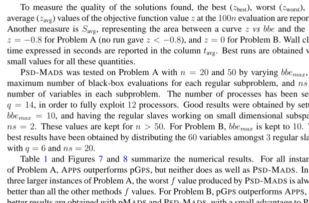
To measure the quality of the solutions found, the best (zbest), worst (zworst), and
average (zavg) values of the objective function valuezat the100nevaluation are reported.
Another measure is Savg, representing the area between a curve z vs bbe and the line z =−0.8for Problem A (no run gavez < −0.8), andz = 0for Problem B. Wall clock time expressed in seconds are reported in the columntavg. Best runs are obtained with
small values for all these quantities.
PSD-MADS was tested on Problem A with n = 20and 50by varying bbemax, the maximum number of black-box evaluations for each regular subproblem, and ns the number of variables in each subproblem. The number of processes has been set to
q = 14, in order to fully exploit 12processors. Good results were obtained by setting
bbemax = 10, and having the regular slaves working on small dimensional subspaces
ns = 2. These values are kept for n > 50. For Problem B, bbemax is kept to10. The best results have been obtained by distributing the60variables amongst3regular slaves withq= 6andns= 20.
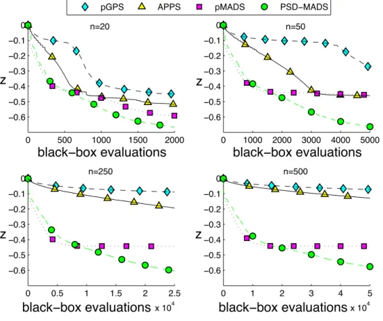
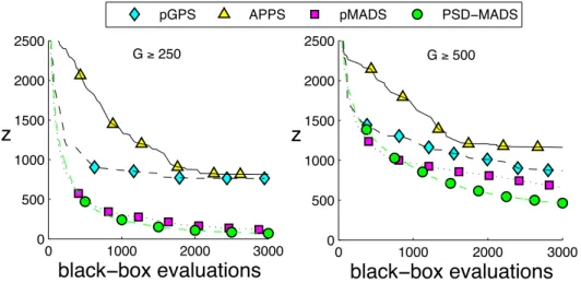
Table 1 and Figures 7 and 8 summarize the numerical results. For all instances of Problem A, APPSoutperforms pGPS, but neither does as well as PSD-MADS. In the three larger instances of Problem A, the worstfvalue produced by PSD-MADSis always better than all the other methodsf values. For Problem B, pGPSoutperforms APPS, and better results are obtained with pMADSand MADS, with a small advantage to PSD-MADS. In all the curves in Figures7 and 8, one can notice that pMADS is always the fastest to descend, but PSD-MADS overtakes it and produces better solutions. Finally, we remark that APPSterminates in the least wall clock time on smaller problems, albeit with a less optimal function value. However for problems with 250 and 500 variables the wall clock time grows significantly worse. This is in accordance with the remark in [25] stating that APPStargets problems with less than 100 variables.
We conclude this section with some advice for readers interested in testing PSD-MADS. First, we think that the PSD-MADS decomposition is beneficial for problems with more than 20 variables. For these problems, at least 3 processors are necessary. Furthermore, since the master and cache server processes are not demanding in terms of cpu, 5 processes can be executed on the 3 processors, whose work will be mainly devoted to two regular slaves and the pollster. Two regular slaves is the minimum number to benefit from the decomposition. So, even if only a few processors are available, it is still worthwhile to try this method. Finally, if the user has no particular strategy to choose the subsets of variables in each subproblem, we recommend to equally distribute the variables to the regular slaves. If the user knows that some of the variables are more likely to produce descent than others, then some subproblems can be devoted to these variables while single-poll MADS can be used on subproblems of less important variables.
0 500 1000 1500 2000 −0.6 −0.5 −0.4 −0.3 −0.2 −0.1 0
black−box evaluations z
n=20
pGPS APPS pMADS PSD−MADS
0 1000 2000 3000 4000 5000 −0.6 −0.5 −0.4 −0.3 −0.2 −0.1 0 n=50
black−box evaluations z 0 0.5 1 1.5 2 2.5 x 10⁴ −0.6 −0.5 −0.4 −0.3 −0.2 −0.1 0 n=250
black−box evaluations z 0 1 2 3 4 5 x 10⁴ −0.6 −0.5 −0.4 −0.3 −0.2 −0.1 0 n=500
black−box evaluations z
Figure 7: Problem A: graphs of the objective function value vs the number of evaluations for all test results. PSD-MADSand pMADSplots correspond to average values of the 30 runs performed for each test.
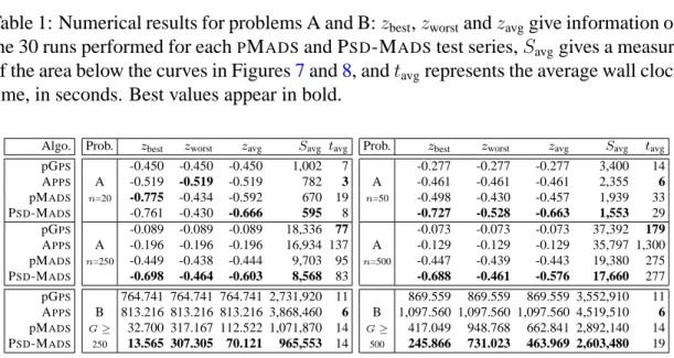
Table 1: Numerical results for problems A and B:zbest,zworstandzavggive information on
the 30 runs performed for eachPMADSand PSD-MADStest series,Savggives a measure
of the area below the curves in Figures7and8, andtavgrepresents the average wall clock
time, in seconds. Best values appear in bold.
Algo. pGPS APPS pMADS PSD-MADS pGPS APPS pMADS PSD-MADS pGPS APPS pMADS PSD-MADS
Prob. zbest zworst zavg Savg tavg
-0.450 -0.450 -0.450 1,002 7 A -0.519 -0.519 -0.519 782 3 n=20 -0.775 -0.434 -0.592 670 19 -0.761 -0.430 -0.666 595 8 -0.089 -0.089 -0.089 18,336 77 A -0.196 -0.196 -0.196 16,934 137 n=250 -0.449 -0.438 -0.444 9,703 95 -0.698 -0.464 -0.603 8,568 83 764.741 764.741 764.741 2,731,920 11 B 813.216 813.216 813.216 3,868,460 6 G≥ 32.700 317.167 112.522 1,071,870 14 250 13.565 307.305 70.121 965,553 14
Prob. zbest zworst zavg Savg tavg
-0.277 -0.277 -0.277 3,400 14 A -0.461 -0.461 -0.461 2,355 6 n=50 -0.498 -0.430 -0.457 1,939 33 -0.727 -0.528 -0.663 1,553 29 -0.073 -0.073 -0.073 37,392 179 A -0.129 -0.129 -0.129 35,797 1,300 n=500 -0.447 -0.439 -0.443 19,380 275 -0.688 -0.461 -0.576 17,660 277 869.559 869.559 869.559 3,552,910 11 B 1,097.560 1,097.560 1,097.560 4,519,510 6 G≥ 417.049 948.768 662.841 2,892,140 14 500 245.866 731.023 463.969 2,603,480 19
6
Discussion and possible extensions
This paper introduced PSD-MADS, a new parallel space decomposition technique with less restrictive conditions than usual PSDmethods on the functions to be optimized and on the sets of variables in the subproblems. A convergence analysis is given based on the Clarke calculus and the MADSconvergence analysis. A practical implementation is described, with a small number of parameters (bbemax and ns), and very encouraging results have been obtained on a difficult problem from the literature, with up to 500 variables.
We presented a first basic implementation of PSD-MADS, with a very simple and generic strategy to choose the sets of variables. An obvious extension is a better strategy to decide on the sets of variables in the subproblems. Of course, it is not clear how to do this in general or we would have done it here. However, for some applications, the user may have special knowledge that would help in this task. For example, the user might put similarly scaled variables in the same subproblem.
It would also be interesting to incorporate the PVDidea of the “forget-me-not” terms, and allow some basic changes in the subproblems for fixed variables. A third possibility would be to perform some additional search steps in the slave subspaces. Another pos-sible extension would be to reintroduce the synchronization step of the original block-Jacobi method, but without the parallel barrier. This “recomposition” step could be performed in parallel by one of the regular slaves, from a pool of successful points, in order to create a problem similar to the one in [19]. Finally, constraints ofΩcould be treated with the progressive barrier [9], instead of the extreme barrier approach. This would allow for infeasible iterates, including the starting point.
0 1000 2000 3000 0 500 1000 1500 2000 2500
black!box evaluations z
G ! 250
pGPS APPS pMADS PSD!MADS
0 1000 2000 3000 0 500 1000 1500 2000 2500 G ! 500
black!box evaluations z
Figure 8: Problem B: graphs of the objective function value vs the number of evaluations for all test results. PSD-MADSand pMADSplots correspond to average values of the 30 runs performed for each test.
Acknowledgment
We would like to thank anonymous referees for their constructive remarks and com-ments.
References
[1] M. A. Abramson. Mixed Variable Optimization of a Load-Bearing Thermal Insulation System Using a Filter Pattern Search Algorithm. Optimization and Engineering, 5(2):157– 177, 2004.
[2] M. A. Abramson and C. Audet. Convergence of Mesh Adaptive Direct Search to Second-Order Stationary Points. SIAMJournal on Optimization, 17(2):606–619, 2006.
[3] P. Alberto, F. Nogueira, U. Rocha, and L. N. Vicente. Pattern Search Methods for user-provided points: application to molecular geometry problems. SIAMJournal on Optimiza-tion, 14(4):1216–1236, 2004.
[4] C. Audet, V. B´echard, and S. Le Digabel. Nonsmooth optimization through Mesh Adap-tive Direct Search and Variable Neighborhood Search. To appear in Journal of Global Optimization, DOI: 10.1007/s10898-007-9234-1, 2007.
[5] C. Audet, G. Couture, and J. E. Dennis, Jr. NOMADproject (LTMADSpackage). Software available atwww.gerad.ca/nomad.
[6] C. Audet, A. L. Cust´odio, and J. E. Dennis, Jr. Erratum : Mesh Adaptive Direct Search Algorithms for Constrained Optimization. SIAM Journal on Optimization, 18(4):1501– 1503, 2008.
[7] C. Audet and J. E. Dennis, Jr. Analysis of Generalized Pattern Searches. SIAMJournal on Optimization, 13(3):889–903, 2003.
[8] C. Audet and J. E. Dennis, Jr. Mesh Adaptive Direct Search Algorithms for Constrained Optimization. SIAMJournal on Optimization, 17(1):188–217, 2006.
[9] C. Audet and J. E. Dennis, Jr.A MADSAlgorithm with a Progressive Barrier for
Derivative-Free Nonlinear Programming. Technical Report G-2007-37, Les Cahiers duGERAD, May 2007.
[10] C. Audet and D. Orban.Finding Optimal Algorithmic Parameters Using the Mesh Adaptive Direct Search Algorithm. SIAMJournal on Optimization, 17(3):642–664, 2006.
[11] D. P. Bertsekas and J. N. Tsitsiklis.Parallel and distributed computation: numerical meth-ods. Prentice-Hall, Inc., Upper Saddle River, NJ, USA, 1989.
[12] A. J. Booker, E. J. Cramer, P. D. Frank, J. M. Gablonsky, and J. E. Dennis, Jr. MOVARS: Multidisciplinary Optimization Via Adaptive Response Surfaces. AIAAPaper 2007–1927, Presented at the 48th AIAA/ASME/ASCE/AHS/ASCStructures, Structural Dynamics, and
Materials Conference, Honolulu, 2007.
[13] A. J. Booker, J. E. Dennis, Jr., P. D. Frank, D. W. Moore, and D. B. Serafini.Managing Sur-rogate Objectives to Optimize a Helicopter Rotor Design – Further Experiments. AIAA Pa-per 1998–4717, Presented at the 8th AIAA/ISSMOSymposium on Multidisciplinary Anal-ysis and Optimization, St. Louis, 1998.
[14] A. J. Booker, J. E. Dennis, Jr., P. D. Frank, D. B. Serafini, V. Torczon, and M. W. Trosset. A Rigorous Framework for Optimization of Expensive Functions by Surrogates. Structural Optimization, 17(1):1–13, February 1999.
[15] F. H. Clarke. Optimization and Nonsmooth Analysis. Wiley, New York, 1983. Reissued in 1990 by SIAM Publications, Philadelphia, as Vol. 5 in the series Classics in Applied Mathematics.
[16] I. D. Coope and C. J. Price. Frame-Based Methods for Unconstrained Optimization. Jour-nal of Optimization Theory and Applications, 107(2):261–274, 2000.
[17] J. E. Dennis, Jr. and V. Torczon. Direct Search Methods on Parallel Machines. SIAM
Journal on Optimization, 1(4):448–474, November 1991.
[18] J. E. Dennis, Jr. and Z. Wu.Parallel continuous optimization, pages 649–670. Sourcebook of parallel computing. Morgan Kaufmann Publishers Inc., San Francisco, CA, USA, 2003. [19] M. C. Ferris and O. L. Mangasarian. Parallel Variable Distribution. SIAM Journal on
[20] D.E. Finkel and C.T. Kelley. Convergence Analysis of the DIRECTAlgorithm. Technical Report CRSC-TR04-28, Center for Research in Scientific Computation, 2004.
[21] K. R. Fowler, C. T. Kelley, C. T. Miller, C. E. Kees, R. W. Darwin, J. P. Reese, M. W. Far-thing, and M. S. C. Reed.Solution of a Well-Field Design Problem with Implicit Filtering. Optimization and Engineering, 5(2):207–234, 2004.
[22] A. Frommer and R. A. Renaut. A Unified Approach to Parallel Space Decomposition Methods. Journal of Computational and Applied Mathematics, 110:205–233, 1999. [23] M. Fukushima. Parallel Variable Transformation in Unconstrained Optimization. SIAM
Journal on Optimization, 8(3):658–672, 1998.
[24] J. Gablonsky and C. T. Kelley.A Locally-Biased Form of the DIRECTAlgorithm. Journal of Global Optimization, 21:27–37, 2001.
[25] G. A. Gray and T. G. Kolda. Algorithm 856: APPSPACK4.0: Asynchronous parallel pat-tern search for derivative-free optimization. ACMTransactions on Mathematical Software, 32(3):485–507, September 2006.
[26] S.-P. Han. Optimization by updated conjugate subspaces. In Numerical analysis (Dundee, 1985), volume 140 of Pitman Res. Notes Math. Ser., pages 82–97. Longman Sci. Tech., Harlow, 1986.
[27] R. E. Hayes, F. H. Bertrand, C. Audet, and S. T. Kolaczkowski. Catalytic Combustion Kinetics: Using a Direct Search Algorithm to Evaluate Kinetic Parameters from Light-Off Curves. The Canadian Journal of Chemical Engineering, 81(6):1192–1199, 2003.
[28] A. Hedar and M. Fukushima. Derivative-free filter simulated annealing method for con-strained continuous global optimization. Journal of Global Optimization, 35(4):521–549, 2006.
[29] P. D. Hough, T. G. Kolda, and V. Torczon. Asynchronous Parallel Pattern Search for Non-linear Optimization. SIAMJournal on Scientific Computing, 23(1):134–156, June 2001. [30] D. R. Jones, C. D. Perttunen, and B. E. Stuckman. Lipschitzian Optimization Without
the Lipschitz Constant. Journal of Optimization Theory and Application, 79(1):157–181, October 1993.
[31] C. T. Kelley. Iterative Methods for Optimization. Number 18 in Frontiers in Applied Mathematics. SIAM, Philadelphia, 1999.
[32] M. Kokkolaras, C. Audet, and J. E. Dennis, Jr. Mixed variable optimization of the num-ber and composition of heat intercepts in a thermal insulation system. Optimization and Engineering, 2(1):5–29, 2001.
[33] T. G. Kolda.Revisiting Asynchronous Parallel Pattern Search for Nonlinear Optimization. SIAMJournal on Optimization, 16(2):563–586, 2005.
[34] T. G. Kolda, R. M. Lewis, and V. Torczon.Optimization by direct search: new perspectives on some classical and modern methods. SIAMReview, 45(3):385–482, 2003.
[35] T. G. Kolda and V. Torczon. Understanding Asynchronous Parallel Pattern Search. In G. DiPillo and A. Murli, editors, High Performance Algorithms and Software for Nonlinear Optimization, pages 316–335. Kluwer Academic Publishers B.V., 2003.
[36] T. G. Kolda and V. Torczon.On the convergence of Asynchronous Parallel Pattern Search. SIAMJournal on Optimization, 14(4):939–964, 2004.
[37] R. M. Lewis and V. Torczon.Pattern Search Algorithms for Bound Constrained Minimiza-tion. SIAMJournal on Optimization, 9(4):1082–1099, 1999.
[38] R. M. Lewis and V. Torczon. Pattern Search Methods for Linearly Constrained Minimiza-tion. SIAMJournal on Optimization, 10(3):917–941, 2000.
[39] R. M. Lewis, V. Torczon, and M. W. Trosset. Direct Search Methods: Then and Now. Journal of Computational and Applied Mathematics, 124(1–2):191–207, December 2000. [40] C.-S. Liu and C.-H. Tseng.Parallel Synchronous and Asynchronous Space-Decomposition
Algorithms for Large-Scale Minimization Problems. Computational Optimization and Ap-plications, 17(1):85–107, 2000.
[41] O. L. Mangasarian. Parallel Gradient Distribution in Unconstrained Optimization. SIAM
Journal on Control and Optimization, 33(6):1916–1925, 1995.
[42] A. L. Marsden, M. Wang, J. E. Dennis, Jr., and P. Moin. Optimal Aeroacoustic Shape Design Using the Surrogate Management Framework. Optimization and Engineering, 5(2):235–262, 2004.
[43] J. A. Nelder and R. Mead. A Simplex Method for Function Minimization. The Computer Journal, 7(4):308–313, January 1965.
[44] C. J. Price and I. D. Coope. Frames and Grids in Unconstrained and Linearly Constrained Optimization: A Nonsmooth Approach. SIAMJournal on Optimization, 14(2):415–438, 2003.
[45] C. A. Sagastiz´abal and M. V. Solodov.Parallel Variable Distribution for Constrained Opti-mization. Computational Optimization and Applications, 22(1):111–131, 2002.
[46] M. V. Solodov. New Inexact Parallel Variable Distribution Algorithms. Computational Optimization and Applications, 7(2):165–182, 1997.
[47] M. V. Solodov. On the Convergence of Constrained Parallel Variable Distribution Algo-rithms. SIAMJournal on Optimization, 8(1):187–196, 1998.
[48] B. Tang. Orthogonal array-based latin hypercubes. Journal of the American Statistical Association, 88(424):1392–1397, 1993.