A Multi-Objective Robust Optimization Model for a Facility Location-Allocation
Problem in a Supply Chain under Uncertainty
S. Mohammad Arabzad
1, Mazaher Ghorbani
2, Sarfaraz Hashemkhani Zolfani
31
Islamic Azad University Tehran, Iran
E-mail. [email protected]
2
Yazd University Yazd, Iran
E-mail. [email protected]
3
Amirkabir University of Technology (Tehran Polytechnic) P.O. Box 1585-4413, Tehran, Iran
E-mail. [email protected]
http://dx.doi.org/10.5755/j01.ee.26.3.4287
The final purpose of this study is presentation a mathematical model for a facility location-allocation problem so as to design an integrated supply chain. A supply chain with multiple suppliers, multiple products, multiple plants, multiple transportation alternatives and multiple customers is taken into account for this purpose. The problem is to specify a number and capacity level of plants, allocation of customers demand, and selection and order allocation of suppliers. A scenario approach is considered to deal effectively with the uncertainty of demand and cost parameters. The formulation is a robust multi-objective mixed-integer linear programming (MOMILP), in the context of which two conflicting objectives is taken into account simultaneously: (1) minimizing the total costs of a supply chain including raw material costs, transportation costs and establishment costs of plants, and (2) minimizing the total deterioration rate occurred by transportation alternatives. Then, the problem can be reduced to a linear one. Finally, by applying the LP-metric method, the model is solved as a single objective mixed-integer programming model. An experiment study corroborates that this procedure can be proposed to design an effective supply chain.
Keywords: Supply chain design, Facility location-allocation, Robust multi-objective optimization, Uncertainty.
Introduction
Many companies struggle with justifying the costs of supply chain (SC) in order to increase the profit achieved by the market share. One of the areas in designing a supply chain is logistics. What many companies fail to see is the coordination and cooperation between logistic issues and supply chain management. In order to create a profitable final product, the company must address all aspects of supply chain, including facility location-allocation.
The area of SCM is a significant issue among authorities which has stimulated a lot of debates. SCM as the process of planning, implementing and controlling the operations of the supply chain desires to meet customer requirements as efficiently and effectively as possible. It spans all movements and storage of raw materials, work-in-process (WIP) inventory, and finished goods from the point-of-origin to the point-of-consumption (Simchi-Levi et al., 2004).
A facility location-allocation problem that has been a well-established research area within operations research (OR), as one of the most noted examples of a supply chain problem, comprises a series of potential facility plants where a facility can be opened and a series of demand points that must be serviced. The goal is to pick a subset of
facilities to open in such a way that the sum of distances from each demand point to its nearest facility and the sum of opening costs of the facilities are minimized. If a supply chain still wants to stay profitable, logistic issues should be regarded as part of a decision making process. The purpose of this article is to model the situation that location and transportation decisions can use to design the optimized supply chain.
Background
production problem (Kanyalkar & Adil, 2005; Liu & Lin, 2005) a capacitated facility location–allocation problem (Liu & Lin, 2005; Amiri, 2006; Torres-Sotoa & Halit, 2011;) and a multi-objective facility location–allocation problem (Bashiri & Hosseininezhad, 2009; Singh & Singh, 2011; Jolai et al., 2011; Zarandi et al., 2011).
Considering the increasing competition between companies, more demanding customers and reduction in profit margin, SCM became an important practice for companies that not only want to stay in business but also have their results optimized and meet the clients’ expectations. Literature about facility location-allocation in supply chain design is extensive and diverse. Historically, researchers have focused relatively early on the design of distribution systems (Lehtonen & Salonen, 2006; Stasiskiene & Sliogeriene, 2009), but without enough considering the supply chain as a whole. Almost 80 percent of the surveyed papers refer to one or two parts of SCM and among these papers; about two thirds model location decisions in only one part (Melo et al., 2009). However, there are some studies considered the whole supply chain in facility location-allocation problem (Sabri & Beamon, 2000; Salema et al., 2006; Yeh, 2006; Manzini & Gebennini, 2008; Samaranayake et al., 2011).
Uncertainty in facility location models
Another characteristic of a facility location-allocation model comes into the equation when various parameters vary throughout the time in a predictable way. They can be placed in the model to get a network design in order to deal effectively with the possible future changes. There are large numbers of deterministic models in comparison with stochastic ones (Melo et al., 2009). According to (Sabri & Beamon, 2000), uncertainty is regarded as one of the most controversial, but significant problems in SCM. Nevertheless, a stochastic environment in combination with location decisions in the context of SCM is still infrequent in the literature. Different sources of uncertainty, such as customer demands, exchange rates, travel times, amount of returns in reverse logistics, supply lead times, transportation costs, and holding costs, have been discussed throughout the literature. (Bar-Lev et al., 1993; Halidias & Michta, 2007; Abiri & Yousefli, 2011; Bartke, 2011; Carmichael & Balatbat, 2011).
Multi-objective optimization with single/multiple
periods and products in facility location models
Most of the existing literature about facility location is focused on the optimization of only one objective; usually cost or profit and other important factors such as deterioration rate with various transportation alternatives (TAs) are left outside the analysis.
There are many techniques for multi-objective optimization such as 𝜀-constrained and LP-metric methods. (Guillen et al., 2005) used the 𝜀-constrained method to make trade-off between three conflicting objectives, profit, demand satisfaction and financial risk cost in a three echelon supply chain. (Mirzapour Al-e-Hashem et al., 2011) utilized LP-metric method to solve a multi-objective aggregation planning in supply chain under
uncertainty with multiple products and multiple periods which minimize the production related costs and total losses of supply chain. This method provides a set of objectives that are Pareto efficient, thus forming a Pareto frontier.
Single/multiple periods and single or multiple products are the other issues that separate a facility location-allocation model, in which most of researches considered single period. Although, a single period facility location model may be enough to find a ‘‘robust” network design (Melo et al., 2009), there are some papers considered multiple periods in production horizon (Ko & Evans, 2007; Hinojosa et al., 2008; Srivastava, 2008; Manzini & Gebennini, 2008; Jolai et al., 2011). In addition, some researchers have taken into account multiple products (Sabri & Beamon, 2000; Ko & Evans, 2007; Hinojosa et al., 2008; Srivastava, 2008; Pati et al., 2008; Manzini & Gebennini, 2008; Kazemi et al., 2009).
For the detailed literature review on facility location– allocation problems, readers are referred to (Drezner & Hamacher 2002; Klose & Drexl, 2005; Melo et al., 2009; Farahani et al., 2010).
Problem statement
Companies must decide on conflicting decisions in supply chain which maximizes the benefit of the whole supply chain as well as minimizing deficiencies. Evaluation of the recent researches on facility location-allocation models in supply chain proves that logistic issues and effects of them are rarely considered in supply chain design.
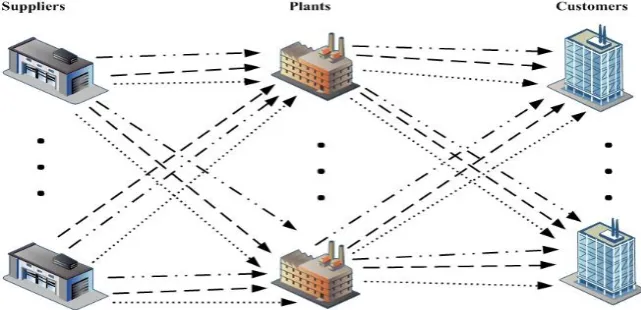
In this paper, we develop a robust optimization program to a facility location-allocation problem to design a supply chain under uncertain customer demands and cost parameters. We consider several suppliers, several plants, and several customer zones with different transportation alternatives (TA). The supply chain produces two kinds of different products to fulfill the customers’ demand, in which the information is given for one period (i.e., planning period). Two conflicting objectives are considered, simultaneously. The first objective aims to minimize the total cost of a supply chain including raw material costs, transportation costs and establishment costs of plants. This objective determines which plants at which a capacity level be opened, allocation of the customers’ demand to the plants and supplier selection and order allocation problem. The second objective tries to minimize the deterioration rate caused by different TAs. Using the LP-metric method, these two objectives are combined, and then the single objective programming is solved. While there is a vast literature devoted on this type of problem, to the best of our knowledge, the majority of researchers consider some of these aspects individually or not considered some of them at all. Furthermore, to enable the model to deal with real situations, different TAs are considered in the whole supply chain. The results show that the proposed model enables decision makers to design an effective supply chain and provide them a global insight to plan for a whole supply chain.
4. Section 5 discusses the results by representing an experiment study. Finally, conclusions and future work are presented in Section 6.
Robust optimization
Two kinds of robustness, namely solution robustness (the solution is nearly optimal in all scenarios) and model robustness (the solution is nearly feasible in all scenarios) were proposed as a framework for robust optimization by (Mulvey et al., 1995). There are two distinct forms of constraints in robust optimization; structural constraint and control constraint. The former is formulated following the concept of linear programming and its input data are free of any noise, while the latter is taken as an auxiliary constraint affected by noisy data (Leung et al., 2007). Moreover, two groups of variables are defined; the design variable which cannot be adjusted once a specific realization of the data, and the control variable which is subject to adjustment once uncertain parameters.
The framework of robust optimization is briefly described as following (Mirzapour Al-e-Hashem et al., 2011): s.t.
where x denotes the vector of decision variables that is determined under the uncertainty of model parameters. B, C and e represent random technological coefficient matrices and right hand side vector, respectively.
Assume a finite set of scenarios { } to model the uncertain parameters. Under each scenario
, we associate the subset { } with the probability of scenario ∑ . Eq. (2) is the structural constraint whose coefficients are fixed and free of noise, whilst Eq. (3) is the control constraint whose coefficients are subject to noise. Also, control variable y, which is subject to adjustment when one scenario is realized, can be denoted as for scenario s. presents the infeasibility of the model under scenario s in a condition that model is infeasible. A robust optimization model is formulated by:
s.t.
There are two terms in the objective function representing solution robustness and model robustness. The first term of the objective function becomes a random variable taking the value with the probability of under scenario s. The second term is a feasibility penalty function, which is used to penalize infeasible solutions under some of the scenarios. (Mulvey et al., 1995) used the following equation to represent solution robustness: ∑ ∑ ( ∑ )
where λ denotes the weight placed on a solution variance, in which the solution is less sensitive to change in the data under all scenarios as λ increases. However, the expression in Eq. (9) involves a complicated term, generating a quadratic form in formulation.
Yu & Li (2000) pointed out that dealing with such problems requires a great deal of computations due to the quadratic term and proposed an absolute deviation instead of the quadratic term, which has the following form:
∑ ∑ | ∑ |
Converting objective (10) from a non-linear to a linear programming model with linear constraints by introducing two non-negative deviational variables, we can solve the problem with less computational efforts (Wagner, 1975). Based on (Leung et al., 2007), instead of minimizing the sum of the absolute deviations in Eq. (10), two deviational variables is minimized subject to the original constrains and additional soft constraints that give positive values of the difference inside the absolute functions. However, (Yu & Li, 2000) stated that this direct linearization approach is largely restricted due to many non-negative deviational variables and constraints introduced. The framework of their model is designed to minimize the objective function as follows: ∑ ∑ [( ∑ ) ] s.t. ∑
It is shown the transformation from quadratic programming in Eq. (9) to the mean absolute deviation minimization problem in Eq. 10 and thus changes from the latter to its linear programming formulation in Eqs. (11) to (13). Using the weight the trade-off between solution robustness and model robustness can be modeled by the MCDM process. According to the above discussions, the objective function can be formulated by (Mirzapour Al-e-Hashem et al., 2011):
∑ ∑ [( ∑ ) ] ∑
Model description
can vary. The problem is to determine the set of plants to be opened and the capacity level of these plants. Also, the quantity of raw materials r provided by supplier j to fulfill requirement of plant i and quantity of end products m
shipped to customers are determined in a way that the total cost and the deterioration rate of transportation are minimized simultaneously. It is worth note that different TAs are allowed in the whole supply chain network.
Figure 1. General schema for a supply chain with different TAs
Indices
;
;
;
;
;
;
;
Parameters
;
;
;
;
;
;
; ;
; ; ;
; ;
;
;
;
;
;
.
Decision variables
;
;
;
Mathematical model
∑ ∑ ∑ ∑ ∑ ∑ ∑ ∑ ∑ ∑ ∑ ∑ ∑ ∑ ∑ ∑ ∑ ∑ ∑ ∑ ∑ ∑ ∑ ∑ ∑ s.t. ∑ ∑ ∑ ∑ ∑ ∑ ∑ ∑ ∑ ∑ ∑ ∑ ∑ ∑ ∑ ∑ ∑ ∑ ∑ ∑The first objective function (Eq. 15) aims to minimize the costs of a supply chain including raw material purchasing cost, raw material transportation cost, end product transportation cost and establishment cost of plants, from which the total sell is deducted. The second objective function (Eq. 16) tries to minimize the total deterioration rates of different TAs. Constraints 17–19 are balance equations for the raw materials, demand of customers and end products. Eq. (20) specifies the maximum available raw material that can be produced by supplier j. Eqs. (21) and (22) defines the relationship between product quantities and capacity level of plants. Eq. (23) ensures that each plant can only have one capacity level. Finally, Eq. (24) specifies the capacity constraint of TAs to transport raw materials and end products.
Robust optimization formulation
The uncertain nature of environment makes the facility location-allocation problems more complex. Incorporating uncertainty into the planning decisions necessarily entails providing overwhelming answers to the following questions respectively (Mirzapour Al-e-Hashem et al., 2011). Firstly, what are the proper approaches to deal
effectively with the uncertain parameters? Different scholars are of the conviction that the main approaches are stochastic programming, fuzzy programming, stochastic dynamic programming and robust optimization (Ben-Tal & Nemirovski, 2000; Bertsimas & Sim, 2006). Secondly, how should the appropriate representation of the uncertain parameters be determined? According to (Gupta & Maranas, 2003), in order to handle the uncertainty inherent in the real world problems, three distinct methods were frequently stated. First, the distribution-based approach, where the normal distribution with specified mean and standard deviation is widely raised for modelling uncertain demands and/or parameters; second, the fuzzy-based approach, there in the forecast parameters are considered as fuzzy numbers with accompanied membership functions; and third, the scenario-based approach, in which several discrete scenarios with associated probability levels are used to describe the expected occurrence of particular outcomes.
According to the model presented by (Mulvey et al., 1995), uncertainty is presented by a set of discrete scenarios (s). Therefore, the proposed robust multi-objective model is presented as follows:
∑
∑ ∑ ∑ ∑
∑ ∑ ∑ ∑
∑ ∑ ∑ ∑
The above terms are defined to ease formulation of robust optimization. In the following, the discussed formulation is presented.
∑ ∑ [ ∑ (
) ] ∑
∑ ∑ [ ∑ ( ) ] ∑
s.t.
∑
∑
∑ ∑
Constraints (17–24).
where is the probability of scenario s. The first and second terms in Eq. (31) and (32) are the mean value and variance of the objective functions, respectively. The last term in Eq. (31) and (32) measures the model robustness with respect to infeasibility associated with control constraint in Eq. (35) under scenario s. Constraints (33) and (34) are auxiliary constraints for linearization defined in Eq. (14). Eq. (35) is a control constraint that its violation is penalized in the objective function. If is greater than , then , while as the amount of is less than , then ∑ .
Solution procedure
The LP-metric method is one of the well-known MCDM methods for solving multi-objective problems with conflicting objectives simultaneously. We use this method to solve the proposed multi-objective mixed-integer linear programming (MOMILP) model with two inconsistent objective functions. First, each objective function is solved separately and then a single objective is reformulated that aims at minimizing the summation of the normalized differences between each objective and the optimal values of them. In our presented model, it is assumed that two objective functions are named and . Based on the LP-metric method, each objective function is solved once separately. Assume that the optimal values are and . Now, the LP-metric objectivefunction can be formulated
by:
[ ]
where is the relative weight of components of the objective function (36) given by the decision makers. The above single objective mixed-integer programming model can be efficiently solved by a linear programming solver.
Computational results
In this section, a hypothetical case is considered to illustrate the applicability of the proposed model to practical problems.
Case description
Table 1
Demand of customer zones and sales price
Scenarios Products
Demand Sales Price
Customer zonec Customer zonec
1 2 3 4 5 1 2 3 4 5
1 1 600 300 200 800 700 35000 30000 31000 32000 30000 2 700 800 700 300 600 40000 41000 42000 42000 42000 2 1 700 500 400 800 700 36000 33000 32000 35000 33000 2 800 900 900 600 800 43000 43000 43000 43000 43000 3 1 900 500 400 900 1000 37000 36000 34000 37000 34000 2 800 1100 900 900 800 45000 45000 45000 44000 45000 Table 2
Transportation cost of products
Scenarios Plants Products
Customer zones
1 2 3 4 5
q1 q2 q1 q2 q1 q2 q1 q2 q1 q2
1 1 1 1375 1848 1485 1903 1199 1749 1232 1760 1353 10000
2 1375 1848 1485 1903 1199 1749 1232 1760 1353 10000
2 1 1474 1892 1595 1749 1419 10000 1485 1760 10000 1595
2 1474 1892 1595 1749 1419 10000 1485 1760 10000 1595
3 1 1342 1925 1309 1815 1485 1639 10000 1870 1210 10000
2 1342 1925 1309 1815 1485 1639 10000 1870 1210 10000
2 1 1 1250 1680 1350 1730 1090 1590 1120 1600 1230 10000
2 1250 1680 1350 1730 1090 1590 1120 1600 1230 10000
2 1 1340 1720 1450 1590 1290 10000 1350 1600 10000 1450
2 1340 1720 1450 1590 1290 10000 1350 1600 10000 1450
3 1 1220 1750 1190 1650 1350 1490 10000 1700 1100 10000
2 1220 1750 1190 1650 1350 1490 10000 1700 1100 10000
3 1 1 1125 1512 1215 1557 981 1431 1008 1440 1107 10000
2 1125 1512 1215 1557 981 1431 1008 1440 1107 10000
2 1 1206 1548 1305 1431 1161 10000 1215 1440 10000 1305
2 1206 1548 1305 1431 1161 10000 1215 1440 10000 1305
3 1 1098 1575 1071 1485 1215 1341 10000 1530 990 10000
2 1098 1575 1071 1485 1215 1341 10000 1530 990 10000
Table 3
Transportation cost of raw materials
Scenarios Suppliers Raw materials
Plants
1 2 3
q1 q2 q1 q2 q1 q2
1 1 1 1023 2750 957 3025 1067 2904
2 1023 2750 957 3025 1067 2904
3 1023 2750 957 3025 1067 2904
4 1023 2750 957 3025 1067 2904
5 1023 2750 957 3025 1067 2904
2 1 1232 10000 1023 2310 1177 1958
2 1232 10000 1023 2310 1177 1958
3 1232 10000 1023 2310 1177 1958
4 1232 10000 1023 2310 1177 1958
5 1232 10000 1023 2310 1177 1958
3 1 1078 2442 1177 10000 1001 2530
2 1078 2442 1177 10000 1001 2530
3 1078 2442 1177 10000 1001 2530
4 1078 2442 1177 10000 1001 2530
5 1078 2442 1177 10000 1001 2530
4 1 10000 2200 1221 3025 1023 2805
2 10000 2200 1221 3025 1023 2805
3 10000 2200 1221 3025 1023 2805
4 10000 2200 1221 3025 1023 2805
5 10000 2200 1221 3025 1023 2805
Table 4
Purchasing cost and capacity of suppliers for raw materials
Suppliers Scenarios Raw material (cost) Raw material (capacity)
1 2 3 4 5 1 2 3 4 5
1 1 16500 11000 5390 3960 6160 9000 8000 7000 12000 9000 2 15000 10000 4900 3600 5600
3 13500 9000 4410 3240 5040
2 1 16335 11550 4950 3520 5390 8000 8000 9000 10000 9000 2 14850 10500 4500 3200 4900
3 13365 9450 4050 2880 4410
3 1 16412 11253 5500 3850 7150 8000 8000 8000 10000 6000 2 14920 10230 5000 3500 6500
3 13428 9207 4500 3150 5850
4 1 14520 8470 5720 3740 4950 8000 8000 8000 10000 9000 2 13200 7700 5200 3400 4500
3 11880 6930 4680 3060 4050 Units of raw materials required for products
Products 1 2 3 4 5
1 3 1 2 1 2
2 2 1 1 1 2
Table 5
Establishment cost and capacity of plants
Scenarios
Plants
1 2 3
n1 n2 n1 n2 n1 n2
1 170000000 230000000 160000000 240000000 160000000 220000000 2 160000000 220000000 150000000 230000000 150000000 210000000 3 150000000 210000000 140000000 220000000 140000000 200000000
Capacity 2000 5000 2000 5000 2000 5000
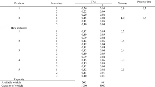
Table 6
Deterioration rate of raw materials and products, capacity of TAs and process time
Products Scenario TAs Volume Process time
1 2
1 1 0,26 0,10 0,9 0,7
2 0,22 0,09
3 0,20 0,08
2 1 0,15 0,08 1,0 0,6
2 0,11 0,05
3 0,10 0,04
Raw materials
1 1 0,12 0,05 0,2
2 0,10 0,03
3 0,09 0,02
2 1 0,14 0,05 0,5
2 0,12 0,04
3 0,11 0,03
3 1 0,12 0,06 0,4
2 0,10 0,05
3 0,09 0,04
4 1 0,15 0,06 0,3
2 0,13 0,05
3 0,12 0,04
5 1 0,12 0,02 0,3
2 0,11 0,01
3 0,10 0,01
Capacity
Available vehicle 200 40
Capacity of vehicle 1000 4000
Based upon the above-mentioned data and taking into account the three scenarios, namely optimistic, realistic and pessimistic with associated probabilities of 0,2, 0,6 and 0,2 respectively, the model is optimally solved three times,
network, the second aims to minimize the expected value and weighted variance of the deterioration rates of products and raw materials, and the last, as the LP-metric objective function, is the best values of the above-mentioned objective functions ( and ).
Computational results
All computations are run using the branch-and-bound algorithm accessed via LINGO 11,0 on a PC Pentium IV-3 GHz and 4 GB RAM DDR under Windows 7. We illustrate the resulted solution, for which we rely on a set of the above-mentioned records in respect of the presented data. Tables 7 to 9 represent the output data characteristics by setting the relative weight ( ) of each objective function component to 0,8 and 0,2 respectively, and the model robustness ( ) to 1000.
Table 7
Production quantity in planning period
Products Plant1 Plant2 Plant3
n1 n2 n1 n2 n1 n2
1 2133 1567
2 800 3700
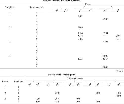
Table 8
Supplier selection and order allocation
Suppliers Raw materials
Plants
1 2 3
q1 q2 q1 q2 q1 q2
1 1
2 200
3 2900
4 5
2 1 7999
2
3 5066 3934
4 2933 5267
5 5866 1534
3 1 4101
2 3 4 5
4 1 8000
2 2733 5267
3 4
5 9000
Table 9
Market share for each plant
Plants Products
Customer zones
1 2 3 4 5
q1 q2 q1 q2 q1 q2 q1 q2 q1 q2
1 1
2
2 1 233 900 1000
2 800
3 1 900 267 400
2 800 1100 900 900
Table 7 presents the set of the selected plants with their relative capacity level and the quantity that should be produced during the planning period. As shown, plant 2
selected suppliers and allocated orders are provided in Table 8. Supplier 2 has the highest share to supply raw materials for these two plants, while supplier 1 has the least share. Table 9 presents the market share of each plant regarding the customer zones.
As stated before, to present the importance of considering three total costs and deterioration rates simultaneously, three following models are extracted for a further analysis.
(1) Model 1 consists of the total costs of the supply chain ( ) subject to the relevant constraints.
(2) Model 2 consists of the sum of the deterioration rates considering TAs ( ) subject to the relevant constraints.
(3) LP-metric model, which is a combination of Model1 and Model2, is calculated by ( ) subject to the relevant constraints.
Thus, changing values of , different solutions for multi-objective optimization is obtained. Figure 2 illustrates the Pareto-optimal frontier for different values of from 0 to 1. It should be noted when , the LP-metric model is equivalent to Model 1, and when , the LP-metric model is equivalent to Model 2.
Figure 2. Trade-off between Z1 and Z2
Considering just one objective may sacrifice the other. Comparison of the results shows that the LP-metric model makes a trade-off between these two objective functions and it is up to the decision maker to select the suitable
from his/her prospective. In Figs. 3 and 4, we discuss the effect to the analysis resulting from changing the value of λ. The following analysis is based on the presented numerical example. The expected cost increases as the value of λ1 is constant and the value of λ2 is increased (see Figure 3). A larger value of λ2 represents a greater importance of deterioration rate variability at the possible expense of the increase of the expected cost. Therefore, the decision maker can get a lower deterioration rate but a higher expected cost results. Comparison of Figs. 3 and 4 also shows the trade-off between the deterioration rate and the expected cost. We can see that with the same value of λ, the lower expected deterioration rate is achieved by increasing the expected cost.
Figure 3. Trade-off between the solution robustness and Z1
Figure 4. Tradeoff between the solution robustness and Z2 It is worth noting that the analysis for a specific example provides some guidance for deciding values of λ for this numerical example. In real cases, some trial experiments can help the decision maker in determining the value of λ.
Conclusion
In this paper, we considered the facility location-allocation problem under the stochastic customer demand and cost parameters to design a supply chain. To handle the uncertainty, we adopted the scenario approach. We integrated the design of a supply chain and production planning for members of the supply chain. A robust optimization formulation was developed for two conflicting mixed-integer linear programming. The first objective was to minimize the costs of supply chain while the second objective intended to minimize the deterioration rate of transportation alternatives. The LP-metric method then was utilized to solve the problem and achieve compromising solution between two objectives. The practicability of the model was demonstrated using an experiment study. The results indicated that the proposed model could provide a promising result to design an efficient supply chain. Selecting optimal location and capacity of the sites, this study also provided selection of the best suppliers and distributors and their allocated order in the supply chain. Moreover, transportation alternatives between the members of the supply chain were selected with regard to minimize costs and failure rates.
Meta-heuristic algorithms are needed to be developed to solve the model for large-scale problems.
In the proposed model, possibility of shortage and surplus are not considered.
The presented model does not consider planning periods. The optimal solution is based on the data of the current period.
In terms of future work, some other issues can be
considered to extend the proposed model, such as scheduling issues. Furthermore, using other approaches to incorporating uncertainty (e.g., fuzzy programming) seems to be interesting. Other extensions for this research work can be considered global issues, such as taxes, tariffs and exchange rates in multiple periods. Employing meta-heuristic algorithms to solve problems in large sizes can also be useful.
References
Abiri, M. B., & Yousefli, A. (2011). An application of possibilistic programming to the fuzzy location–allocation problems. International Journal of Advanced Manufacturing Technology, 53(9/12), 1239–1245. http://dx.doi.org/10. 1007/s00170-010-2896-8
Amiri, A. (2006). Designing a distribution network in a supply chain system: Formulation and efficient solution procedure. European Journal of Operational Research, 171, 567–576. http://dx.doi.org/10.1016/j.ejor.2004.09.018
Bar-Lev, Sh., Parlar, M., & Perry, D. (1993). Impulse control of a brownian inventory system with supplier uncertainty. Stochastic Analysis and Applications, 11(1), 11–27. http://dx.doi.org/10.1080/07362999308809298
Bartke, S. (2011). Valuation of market uncertainties for contaminated land. International Journal of Strategic Property Management, 15(4), 356–378. http://dx.doi.org/10.3846/1648715X.2011.633771
Bashiri, M., & Hosseininezhad, S. J. (2009). A fuzzy group decision support system for multifacility location problems. International Journal of Advanced Manufacturing Technology, 42(5/6), 533–543. http://dx.doi.org/10.1007/s00170-008-1621-3
Ben-Tal, A., & Nemirovski, A. (2000). Robust solutions of linear programming problems contaminated with uncertain data. Mathematical Programming, 88(3), 411–424. http://dx.doi.org/10.1007/PL00011380
Bertsimas, D., & Sim, M. (2006). Tractable approximations to robust conic optimization problems. Mathematical Programming, 107(1), 5–36. http://dx.doi.org/10.1007/s10107-005-0677-1
Carmichael, D., & Balatbat, M. (2011). On the analysis of property unit sales over time. International Journal of Strategic Property Management, 15(4), 329–339. http://dx.doi.org/10.3846/1648715X.2011.631765
Cooper, L. (1963). Location–allocation problems. Operations Research, 11, 331–343. http://dx.doi.org/10.1287/opre.11.3.331 Drezner, Z. & Hamacher, H. W. (2002). Facility location: Applications and theory. Springer.
http://dx.doi.org/10.1007/978-3-642-56082-8
Farahani R. Z., Steadie Seifi. M., & Asgari N. (2010). Multiple criteria facility location problems: A survey. Applied Mathematical Modelling, 34, 1689–1709. http://dx.doi.org/10.1016/j.apm.2009.10.005
Guillen, G., Mele, F. D., Bagajewicz, M. J., Espuna, A., & Puigjaner, L. (2005). Multi-objective supply chain design under uncertainty. Chemical Engineering Science, 60, 1535–1553. http://dx.doi.org/10.1016/j.ces.2004.10.023
Gupta, A., & Maranas C. D. (2003). Managing demand uncertainty in supply chain planning. Computers and Chemical Engineering, 27(8), 1219–1227. http://dx.doi.org/10.1016/S0098-1354(03)00048-6
Halidias, N., & Michta, M. (2007). The Method of Upper and Lower Solutions of Stochastic Differential Equations and Applications. Stochastic Analysis and Applications, 26(1), 16–28. http://dx.doi.org/10.1080/07362990701670217 Hinojosa, Y., Kalcsics, J., Nickel, S., Puerto, J., & Velten, S. (2008). Dynamic supply chain design with inventory.
Computers & Operations Research, 35 373–391. http://dx.doi.org/10.1016/j.cor.2006.03.017
Jiang, J. L., & Yuan, X. M. (2008). A heuristic algorithm for constrained multi-source Weber problem – The variational inequality approach. European Journal of Operational Research, 187, 357–370. http://dx.doi.org/10. 1016/j.ejor.2007.02.043
Jolai, F., Tavakkoli-Moghaddam, R., & Taghipour, M. (2012). A multi-objective particle swarm optimisation algorithm for unequal sized dynamic facility layout problem with pickup/drop-off locations. International Journal of Production Research, 50(15), 4279–4293. http://dx.doi.org/10.1080/00207543.2011.613863
Kanyalkar, A. P., & Adil, G. K. (2005). An integrated aggregate and detailed planning in a multi-site production environment using linear programming. International Journal of Production Research, 43(20), 4431–4454. http://dx.doi.org/10. 1080/00207540500142332
Kazemi, A., Fazel Zarandi, M. H., & Moattar-Husseini S. M. (2009). A multi-agent system to solve the production– distribution planning problem for a supply chain: a genetic algorithm approach. International Journal of Advanced Manufacturing Technology, 44(1/2), 180–193. http://dx.doi.org/10.1007/s00170-008-1826-5
Ko, H. J., & Evans, G. W. (2007). A genetic algorithm-based heuristic for the dynamic integrated forward/reverse logistics network for 3PLs. Computers & Operations Research, 34, 346–366. http://dx.doi.org/10.1016/j.cor.2005.03.004 Lehtonen, T., & Salonen, A. (2006). An empirical investigation of procurement trends and partnership management in FM.
International Journal of Strategic Property Management, 10(2), 65–78.
Leung, S. C. H., Tsang, S. O. S., Ng, W. L., & Wu, Y. (2007). A robust optimization model for multi-site production planning problem in an uncertain environment. European Journal of Operational Research, 181 (1), 224–238. http://dx.doi.org/10.1016/j.ejor.2006.06.011
Liu, S. C., & Lin, C. C. (2005). A heuristic method for the combined location routing and inventory problem. International Journal of Advanced Manufacturing Technology, 26(4), 372–381. http://dx.doi.org/10.1007/s00170-003-2005-3 Manzini, R., & Gebennini, E. (2008). Optimization models for the dynamic facility location and allocation problem.
International Journal of Production Research, 46(8), 2061–2086. http://dx.doi.org/10.1080/00207540600847418 Melo, M. T., Nickel, S., & Saldanha-da-Gama, F. (2009). Facility location and supply chain management – A review.
European Journal of Operational Research, 196, 401–412. http://dx.doi.org/10.1016/j.ejor.2008.05.007
Mirzapour Al-e-Hashem, S. M. J., Malekly, H., & Aryanezhad, M. B. (2011). A multi-objective robust optimization model for multi-product multi-site aggregate production planning in a supply chain under uncertainty. International Journal of Production Economics, 37 (4), 668–683. http://dx.doi.org/10.1016/j.ijpe.2011.01.027
Mulvey, J. M., Vanderbei, R. J., & Zenios, S. A. (1995). Robust optimization of large-scale systems. Operations Research, 43 (2), 264–281. http://dx.doi.org/10.1287/opre.43.2.264
Pati, R. K., Vrat, P., & Kumar, P. (2008). A goal programming model for paper recycling system, Omega, 36 405–417. http://dx.doi.org/10.1016/j.omega.2006.04.014
Sabri, E. H., & Beamon, B. M. (2000). A multi-objective approach to simultaneous strategic and operational planning in supply chain design, Omega, 28, 581–598. http://dx.doi.org/10.1016/S0305-0483(99)00080-8
Salema, M. I., Povoa, A. P. B., & Novais, A.Q. (2006). A warehouse-based design model for reverse logistics. Journal of the Operational Research Society, 57, 615–629. http://dx.doi.org/10.1057/palgrave.jors.2602035
Salema, M. I., Povoa, A. P. B., & Novais, A. Q. (2007). An optimization model for the design of a capacitated multi-product reverse logistics network with uncertainty. European Journal of Operational Research, 179, 1063–1077. http://dx.doi.org/10.1016/j.ejor.2005.05.032
Samaranayake, P., Laosirihongthong, T., & Chan, F. T. S. (2011). Integration of manufacturing and distribution networks in a global car company – network models and numerical simulation. International Journal of Production Research, 49(11), 3127–3149. http://dx.doi.org/10.1080/00207541003643164
Simchi-Levi, D., Kaminsky, P., & Simchi-Levi, E. (2004). Managing the supply chain: The definitive guide for the business professional, McGraw-Hill, New York.
Singh, S. P., & Singh, V. K. (2011). Three-level AHP-based heuristic approach for a multi-objective facility layout problem. International Journal of Production Research, 49(4), 1105-1125. http://dx.doi.org/10.1080/00207540903536148 Srivastava, S. K. (2008). Network design for reverse logistics, Omega, 36, 535–548. http://dx.doi.org/10.1016/
j.omega.2006.11.012
Stasiskiene, Z., & Sliogeriene, J. (2009). Sustainability assessment for corporate management of energy production and supply companies for Lithuania. International Journal of Strategic Property Management, 13(1), 71–81. http://dx.doi.org/10.3846/1648-715X.2009.13.71-81
Torres-Sotoa, J. E., & Halit, U. (2011). Dynamic-demand capacitated facility location problems with and without relocation. International Journal of Production Research, 49(13), 3979–4005. http://dx.doi.org/10.1080/00207 543.2010.505588
Wagner, H. M. (1975). Principles of operations research, 2nd Ed., Prentice Hall, New Jersey.
Yeh, W. C. (2005). A hybrid heuristic algorithm for the multistage supply chain network problem. International Journal of Advanced Manufacturing Technology, 26(5/6), 675–685. http://dx.doi.org/10.1007/s00170-003-2025-z
Yeh, W. C. (2006). An efficient memetic algorithm for the multi-stage supply chain network problem. International Journal of Advanced Manufacturing Technology, 29(7/8), 803–813. http://dx.doi.org/10.1007/s00170-005-2556-6
Yu, C. S., & Li, H. L. (2000). A robust optimization model for stochastic logistic problems. International Journal of Production Economics, 64(1/3), 385–397. http://dx.doi.org/10.1016/S0925-5273(99)00074-2
Zarandi, M. H. F., Sisakht, A. H., & Davari, S. (2011). Design of a closed-loop supply chain (CLSC) model using an interactive fuzzy goal programming. International Journal of Advanced Manufacturing Technology, 56(5/8), 809– 821. http://dx.doi.org/10.1007/s00170-011-3212-y