Annales Geophysicae, 23, 3035–3042, 2005 SRef-ID: 1432-0576/ag/2005-23-3035 © European Geosciences Union 2005
Annales
Geophysicae
One-step ahead prediction of
f o
F2 using time series forecasting
techniques
K. Koutroumbas and A. Belehaki
National Observatory of Athens, Institute for Space Applications and Remote Sensing, Metaxa and V. Pavlou, Palaia Penteli, 15 236, Athens, Greece
Received: 24 February 2005 – Revised: 9 September 2005 – Accepted: 4 October 2005 – Published: 22 November 2005 Part of Special Issue “1st European Space Weather Week (ESWW)”
Abstract. In this paper the problem of one-step ahead prediction of the critical frequency (f oF2) of the middle-latitude ionosphere, using time series forecasting methods, is considered. The whole study is based on a sample of about 58 000 observations off oF2 with 15-min time resolution, derived from the Athens digisonde ionograms taken from the Digisonde Portable Sounder (DPS4) located at Palaia Penteli (38◦N, 23.5◦E), for the period from October 2002 to May 2004. First, the embedding dimension of the dynamical sys-tem that generates the above sample is estimated using the false nearest neighbor method. This information is then uti-lized for the training of the predictors employed in this study, which are the linear predictor, the neural network predictor, the persistence predictor and thek-nearest neighbor predic-tor. The results obtained by the above predictors suggest that, as far as the mean square error is considered as performance criterion, the first two predictors are significantly better than the latter two predictors. In addition, the results obtained by the linear and the neural network predictors are not signif-icantly different from each other. This may be taken as an indication that a linear model suffices for one step ahead pre-diction off oF2.
Keywords. Ionosphere (Modelling and forecasting) –
His-tory of geophysics (Instruments and techniques)
1 Introduction
The accurate prediction of ionospheric conditions is critical for several applications affected by the space weather, in-cludingH F communications, satellite positioning and nav-igation applications. Ionospheric storms can cause large-scale, drastic changes to the usable range ofH F frequen-cies. Large solar flares cause short-wave fadeouts, resulting in blackouts ofH F signals. Also, protons emitted from the Sun result in polar cap absorption events and consequently
Correspondence to: K. Koutroumbas
in blackouts ofH F signals propagating through the Earth’s polar regions. Ionospheric effects can also generate time-varying ionospheric currents, especially in the northern lati-tudes causing problems in ground systems, such as systems for power generation and supply; oil and gas pipeline distri-bution; aerial surveying for minerals, oil and gas; drilling for oil and gas; railways.
To handle the complexity of the problem, the development of accurate models to forecast the ionospheric conditions is of crucial importance, especially during disturbed condi-tions. Considerable effort has been devoted on the develop-ment of physical models (Anderson et al., 1998) based on the coupling between the thermosphere and the ionosphere. However, the use of such models is not suitable for real-time applications due to both the input data requirements for the simulation of the thermosphere (Fuller-Rowell and Rees, 1980) and the computational load.
The empirical models driven by magnetic indices are a second group of ionospheric models. Fuller-Rowell et al. (2001) developed the empirical storm-time ionospheric correction model driven by the previous time-history of the geomagnetic index,ap, and it is designed to scale the quiet-timeF-layer critical frequency (f oF2) to account for storm-time changes in the ionosphere. The model provides a use-ful, yet simple tool for estimating the changes to ionosphere in response to geomagnetic activity.
Another well-known statistical model for the prediction of ionospheric parameters was introduced by Muhtarov and Ku-tiev (1999), which makes use of the auto correlation function of the parameter under consideration without using any geo-magnetic index. Muhtarov et al. (2002) further improved the prediction capability of the autocorrelation model by adding a geomagnetic index and its statistical characteristics.
3036 K. Koutroumbas and A. Belehaki: One-step ahead prediction off oF2 using time series forecasting techniques b; Wintoft and Cander, 2000; McKinnell and Poole, 2000).
Wintoft and Cander (2000) used time-delay, feed-forward neural networks to predict the hourly values of the iono-sphericF2 layer critical frequency,f oF2, 24 h ahead. The 24 measurements off oF2 per day are reduced to five coeffi-cients with principal component analysis. A time delay line of these coefficients is then used as input to a feed-forward neural network. Also included in the input are the 10.7-cm solar flux and the geomagnetic indexAp. The network is
trained usingf oF2 data from 1965 to 1985 gathered at the Slough ionospheric station and validated on an independent validation set from the same station for the periods 1987– 1990 and 1992–1994.
In a recent study, Tulunay et al. (2004) presented the appli-cation of the Middle East Technical University Neural Net-work (METUNN) to forecast thef oF2 values one hour in advance, based on hourly resolution data. The input param-eters are year, month, coded season, day, hour, coded hour, f oF2 value observed one hour ago, first and second rela-tive difference, station code. The method was applied to data from Poitier, Slouth and Uppsala, and the mean square errors were within reasonable limits (0.11353 to 0.21145 MHz).
The problem considered in this study is the estimation of the next value off oF2 using time series forecasting meth-ods. The available data sampleX={x1, x2, . . ., xp}consists
of aboutp=58 000 observations off oF2 derived from the Athens digisonde ionograms taken from the ionospheric sta-tion located at Palaia Penteli, for the period from October 2002 to May 2004. The sampling rate is 15 min. There is a small fraction of missing observations that have been ne-glected from the subsequent prediction stages.
If we denote the current value off oF2 byx(n), then the estimation of the next valuex(n+1)is based on
y(n)= [x(n), x(n−1), . . . , x(n−(d−1))]T. (1) The first problem to be faced is the estimation ofd, the so-called embedding dimension. This is estimated using the
false nearest neighbor method. After the determination of
d, two sets of pairs of the form(y(n), x(n+1))are created. The first one, denoted byS1and called the training set, will
be used for the training of the predictors, while the second one, denoted byS2and called the test set, will be used for
the evaluation of the performance of the predictors. The eval-uation criterion for the above predictors is the mean square
error (MSE), that is the mean value of the squared difference
between the actual and the predicted values off oF2. In this study, both parametric and non-parametric predic-tors are used. Specifically, from the first category the linear predictor, as well as neural network predictors, are consid-ered, while from the second category the persistence predic-tor, as well as theknearest neighbor predictor, are consid-ered. The experimental results show that all predictors ex-hibit a less than 13% error on the test set, in terms of the MSE criterion. This issue will be discussed further in the simulation results section.
The rest of the paper is organized as follows. In Sect. 2, the definition of the embedding dimension,d, is given, together
with a short description of the false nearest neighbor method that estimatesd. In Sect. 3 a short description of the predic-tors considered in this study is given. In Sect. 4 the procedure that generates the training and the test sets,S1andS2, is
de-scribed. In addition, the results of the predictors followed by a short discussion are provided. Finally, concluding remarks, as well as future research directions, are included in Sect. 5.
2 The embedding dimension
LetAdenote thed-dimensional dynamical system that pro-duces the available time series of observations and lets(n) denotes its state vector at time n. Assuming that A is a discrete dynamical system, it is described by the following equation (also called map)
s(n+1)=h(s(n)). (2)
Clearly, this system is unknown, that is we do not know the dimensiond, nor the functionh. The only available informa-tion about it is through the sequence of observainforma-tions{x(n)}, which are related with the state vectors(n)via the following equation:
x(n)=g(s(n)). (3)
Since, in general, the available sequence of observations1 does not represent properly the multi-dimensional phase space of the dynamical system, one has to employ some technique to unfold the multi-dimensional structure using the available data series (Hegger et al., 1999).
The most important technique for the phase space recon-struction is the method of delays (see, e.g. Tsonis, 1992; Hegger et al., 1999). According to this method, the vectors in the new space (the embedding space) are formed from time delayed values of the scalar measurements, i.e.2
y(n)=[x(n), x(n−1), . . ., x(n−(d−1))]T, (4) andd is the dimension of the embedding space, called the embedding dimension. Knowledge ofd is of crucial impor-tance, but, of course, it is unavailable in real world situations and has to be estimated from the available data series. Specif-ically,d should be chosen large enough to allow for the un-folding of the multi-dimensional structure of the system, but not too large, in order to avoid the undesirable effects of the
1which is one-dimensional in most cases
2In general, y(n) is defined as y(n)=[x(n), x(n−T ), . . .,
K. Koutroumbas and A. Belehaki: One-step ahead prediction off oF2 using time series forecasting techniques 3037 noise encountered in the measurements, as well as the
un-necessary increase in computational complexity (Kennel et al., 1992).
A method that has been extensively used for the estima-tion of d is the so-called method of false nearest neigh-bors (Kennel et al., 1992), which is described below. Let X0={x(1), x(2), . . ., x(q)}3 be the set of observations on which the estimation ofd will be based.
The false nearest neighbor method • Compute the quantities
x=1 q
q X
n=1
x(n), RA2=1 q
q X
n=1
(x(n)−x)2.
• SetRtot=15 andAtot=2 (as suggested in Kennel et al.,
1992).
• Choose a high enough value ofd, say,dmax, and useX0
to construct the set
Z= {y(n)=[x(n), x(n−1), . . ., x(n−(dmax−1))]T,
n =dmax, . . ., q}.
• Ford=1 todmax
– For each y(n) inZ, determine its nearest neigh-bor y0(n)=[x0(n), . . . , x0(n−(dmax−1))]T in
Z−{y(n)}, based on the last d coordinates of the y values, i.e. choose y’(n) such that d(y(n),y0(n))=miny∈Z−{y(n)}d(y(n),y), where the distance between two dmax
-dimensional vectors, u and v, is defined as d(u,v)=Pd
i=0(ui−vi)2, whereui andvi are the
i-th coordinates ofuandv, respectively.
– For eachy(n)inZcompute Rd2(n)=Pd−1
k=0(x(n−(dmax−1)+k)
−x0(n−(dmax−1)+k))2
Td2+1(n)= |x(n−(dmax−1)+d)
−x0(n−(dmax−1)+d)|
Rd2+1(n)=Rd2(n)+Td2+1(n)
– Count the points for which
(Td+1(n) Rd(n)
>Rtot)OR(
Rd+1
RA
>Atot)
– If their fraction is smaller than 1% of q (as sug-gested in Kennel et al., 1992), choosed as the em-bedding dimension and terminate the procedure. • End{for-loop}
3We useqinstead ofpobservations for the estimation ofd
be-cause a part of the data will be used for the evaluation of the results obtained by the various predictors, and it is assumed to be unknown.
In words, the above method tests ifdis an appropriate es-timate for the embedding dimension, by utilizing the neigh-borhood information of thedmax-dimensional vectorsy(n)in
Z. Specifically, for each vectory(n)inZ, its nearest neigh-bory0(n)is determined based on the lastdcoordinates of the vectors. LetRd2(n)be the distance betweeny(n)andy0(n) when only the lastdcoordinates are taken into account. Then Rd2+1(n)is computed and the difference betweenRd2(n)and Rd2+1(n)is considered. IfRd2(n)andRd2+1(n)differ signif-icantly, then we say that y0(n) is a false nearest neighbor ofy(n)4. If this happens for a significant number of points y(n)∈Z, it is an indication that the multi-dimensional struc-ture of the system does not “unfold” well in the d dimen-sional space, i.e. a larger value ofdmust be considered.
Finally, it is worth noting that the above algorithm may also be used by considering not only the nearest neighbor of each vectory∈Zbut also itsk-nearest neighbors.
3 The predictors
3.1 Parametric predictors 3.1.1 The linear predictor
In this framework, the estimation of x(n+1), denoted by x(nˆ +1), is assumed to depend linearly on the values x(n), x(n−1), . . . , x(n−(d−1)), i.e.
ˆ
x(n+1)=
d−1
X
i=0
wix(n−i)+wd= [y(n)1]Tw, (5)
wherew=[w0, w1, . . . , wd−1, wd]T is the parameter vector
of the predictor. Given a data setY = {x(1), . . . , x(q)},wis chosen such that the following cost function is minimized
J (w)=
q−d
X
n=d
(x(n+1)− ˆx(n+1))2
=
q−d
X
n=d
(x(n+1)− [y(n)1]Tw)2. (6)
It can be proven (see, e.g. Theodoridis et al., 2003) that the vectorwthat minimizesJ (w)is
ˆ
w=(ZTZ)−1ZTu, (7)
where ZT=[[y(d)T 1]T, [y(d + 1)T 1]T, . . . , [y(q − d)T 1]T]andu=[x(d+1), x(d+2), . . . , x(q−d+1)]T. The estimated value of x(n+1),x(nˆ +1), is given by Eq. (5), wherewˆ is used in place ofw.
4Consider, for example, the points y
1=[0.5, 0.5]T and
3038 K. Koutroumbas and A. Belehaki: One-step ahead prediction off oF2 using time series forecasting techniques 3.1.2 Neural networks predictor
In this study we consider only two-layer, feedforward neural networks (2LF N N), withmnodes in their hidden layer and a single output node5. These networks are modelled by the following equation
ˆ x=g(
m X
j=1
vjf (wjT[yT 1]T)+v0), (8)
whereyis the input vector andxˆis the output of the network. f is typically chosen to be equal to logi(x)=1/(1+e−ax)or tanh(x)=(1−e−ax)/(1+e−ax), whilegmay be chosen to be equal tox, logi(x)or tanh(x). Them (d+1)-dimensional vectors wj, as well as the values of vj, j=0, . . . , m are
the parameters of the network. Let W denote a vector that contains all these parameters. W is usually estimated by optimizing an appropriately defined cost function, using tools from nonlinear optimization theory. Given a data set Y={x(1), . . . x(q)}, a typical cost function that is frequently employed is the sum of square errors, defined as
J (W)= q−d
X
n=d
(x(n+1)−g
m
X
j=1
vjf (wjT[yT(n)1]T)+v0)
!2 . (9)
The advantage of the above types of models is that they can describe more reliably phenomena that exhibit significant nonlinearities. However, their major disadvantage follows from the fact that the cost function to be optimized is non-convex, due to the nonlinear nature off and (probably)gin Eq. (8). As a consequence, it is difficult to obtain the global optimumW∗ofJ (W)that best represents the data at hand. Thus, instead of trying to determine the global optimum of J (W), we seek for local optima ofJ (W), which are (hope-fully) suitable for the problem at hand. Their suitability is assessed through the test set.
3.2 Non-parametric predictors 3.2.1 The persistence predictor
In this case, the estimator ofx(n+1),x(nˆ +1), isx(n), that isx(nˆ +1)=x(n). This simple predictor is expected to give satisfactory results in cases where the sample-to-sample vari-ation is small, as is the case for periods where no significant disturbances occur in the ionosphere.
3.2.2 Theknearest neighbor predictor
In this case, for a given vectory(n), the predictor computes the estimate ofx(n+1)as follows. First, theknearest neigh-bors, denoted byy(n1),y(n2), . . . ,y(nk), ofy(n)inS1are
identified. Then, the estimate ofx(n+1)is taken to be equal to the mean ofx(n1+1), x(n2+1), . . . , x(nk +1). This
method is met under the name “first order local approxima-tion” in Tsonis (1992).
5See, e.g. Rummelhart et al. (1986); Pao (1989); Haykin (1994);
Theodoridis et al. (2003).
20
dimension
Percentage
of
false
nearest
neighbors
1 2 3 4 5 6 7
0 0.1 0.2 0.3 0.4 0.5 0.6 0.7 0.8 0.9
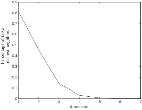
[image:4.595.311.545.63.244.2]Figure 1:
Fig. 1. Plot of the percentage of the false nearest neighbors versus
the space dimension. For dimensions greater than or equal to 6 the percentage falls well below 1%.
4 Experimental results
Before we proceed with the generation of the training and the test sets, we need to estimate the embedding dimension dof the space where the dynamical system that produces the data sample X at hand “unfolds” in a satisfactory fashion its multi-dimensional structure. In applying the false nearest neighbor method described in Sect. 2 at the first half of the data sampleX(that isq=p/2), we find that a good choice for d is 6. Specifically, for dimensions greater than or equal to 6, the percentage of false nearest neighbors falls well below 1% (see also Fig. 1)6.
Having estimatedd, we then describe the way the training and the test sets are generated. Specifically, the data sam-pleXis split into two halves,X1(first half) andX2(second
half). From eachXi,i=1,2, a corresponding setSi,i=1,2
is generated as follows S1= {(y(d), x(d+1)),
(y(d+1), x(d+2)), . . . , (y(p/2−1), x(p/2))}(10) and
S2= {(y(p/2+d), x(p/2+d+1)), (y(p/2+d+1),
x(p/2+d+2)), . . . , (y(p−1), x(p))}, (11) where d is chosen to be equal to 6, y(n) is defined as in Eq. (1) and the vectorsy(n)with missing values are omitted. All the predictors have been trained usingS1, and their
performance has been measured on the test setS2. The
re-sults are summarized in Table 1. Also, in Figs. 2, 3, 4 and 5 the histogram of the absolute differences between the ac-tual and the estimated values on the test set, as well as the plot of the actual and the predicted values for a short time
6We note that the same value fordis taken if we consider the
K. Koutroumbas and A. Belehaki: One-step ahead prediction off oF2 using time series forecasting techniques 3039
Table 1. Fifteen-minute ahead prediction. The table shows the mean square error on the training set and on the test set for the linear
predictor, the 2LFNN predictor with 4 nodes in the hidden layer, the persistence predictor and thek-nearest neighbor predictor, fork=12. In parentheses the standard deviation of the squared errors for each predictor on the test set is shown.
Linear 2LF N Npredictor Persistence k-nearest neighbor predictor (nodes=4) predictor predictor (k=12)
Training set 0.1599 0.1462 0.1780 0.1311
Test set 0.1105 0.1050 0.1253 0.1272
(0.3041) (0.2879) (0.3144) (0.3165)
21
0 0.5 1 1.5 2 2.5 3 3.5 4 4.5 0
500 1000 1500 2000 2500 3000 3500 4000 4500
600 650 700 750 800 850
4 5 6 7 8 9 10
a) ( Absolute error
Number
of
samples
b) ( Time
FoF2
value
Figure 2:
21
0 0.5 1 1.5 2 2.5 3 3.5 4 4.5 0
500 1000 1500 2000 2500 3000 3500 4000 4500
600 650 700 750 800 850
4 5 6 7 8 9 10
a) ( Absolute error
Number
of
samples
b) ( Time
FoF2
value
Figure 2:
Fig. 2. One-step ahead (15 min) prediction, with the linear predictor. (a) The histogram of the absolute differences of the computed and the
actual outputs, for the test set. (b) The actual (solid line) and the computed (dotted line) outputs for a short time interval of the test set.
interval, are given for each of the four predictors. It is noted that various 2LF N N architectures with different numbers of hidden layer nodes have been examined. Specifically, 2LF N Ns with up tom=50 nodes in the hidden layer have been considered. However, the best performance was ob-tained form=4 nodes. We also note that the mean square error (MSE) value for the 2LF N Ns, shown in Table 1, is the average of the MSEs of 10 networks, withm=4 hidden nodes, that have been trained with the Levenberg-Marquardt algorithm starting from different initial values for the param-eters. Also, for thek-nearest neighbor predictor, the results fork=1,2, . . . ,30 have been considered. Here, only the best results are provided.
As can be seen from the results shown in Table 1 (and sup-ported by Figs. 2, 3, 4 and 5), all predictors seem to exhibit more or less a similar performance. However, in order to quantify the significance of the differences among the mean square errors (MSE) produced by any pair of the above clas-sifiers when they are applied on the test set, we use thet-test statistic (see, e.g. Mendenhall et al., 1995). The choice of this test is justified by the fact that the errors produced by
the predictors are independent, since each one of the predic-tors follows a different prediction strategy from all the oth-ers. More specifically, for any two of the above predictors,
P1andP2, we test the hypothesis
H0: MSE1−MSE2=0
against
H1: MSE1−MSE2>0,
where MSEi is the mean square error (MSE) forPi,i=1,2.
Denoting the sample MSE forPi (as it is given in Table 1) by MSEi and assuming that MSE1>MSE2, we compute the
quantity
z=MSE1−MSE2
q
s2
1+s22 n
, (12)
where si is the sample data deviation of the squared errors
produced byPi, andnis the number of samples (in our case
3040 K. Koutroumbas and A. Belehaki: One-step ahead prediction off oF2 using time series forecasting techniques
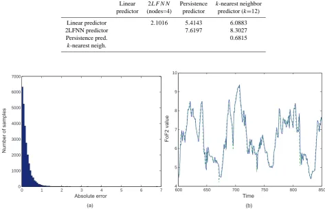
Table 2. Fifteen-minute ahead prediction. The table shows the values of thet-test that quantify the significance of the differences in the mean square error produced by two predictors when the test set is considered.
Linear 2LF N N Persistence k-nearest neighbor predictor (nodes=4) predictor predictor (k=12)
Linear predictor 2.1016 5.4143 6.0883
2LFNN predictor 7.6197 8.3027
Persistence pred. 0.6815
k-nearest neigh.
22
a) ( Absolute error
Number
of
samples
b) ( Time
FoF2
value
0 1 2 3 4 5 6 7
0 1000 2000 3000 4000 5000 6000 7000
600 650 700 750 800 850
4 5 6 7 8 9 10
Figure 3:
22
a) ( Absolute error
Number
of
samples
b) ( Time
FoF2
value
0 1 2 3 4 5 6 7
0 1000 2000 3000 4000 5000 6000 7000
600 650 700 750 800 850
4 5 6 7 8 9 10
Figure 3:
Fig. 3. One-step ahead (15 min) prediction, with the 2LF N N model with 4 nodes. (a) The histogram of the absolute differences of the computed and the actual outputs, for the test set. (b) The actual (solid line) and the computed (dotted line) outputs for a short time interval of the test set.
0.01 and taking into account the above value ofn, the value za for thet-test is 2.326. Recalling that theH0hypothesis
is rejected whenz>za, the values in the table lead to the
following conclusions:
– At significance level 0.01, there is not enough sufficient evidence to reject the hypothesis that the MSE for the linear predictor and neural network predictor are equal7.
– At significance level 0.01, there is not enough sufficient evidence to reject the hypothesis that the MSE for the persistence predictor andk-nearest neighbor predictor are equal.
– At significance level 0.01, the MSEs for the non-parametric predictors differ significantly from the MSEs for the parametric predictors.
Adopting the Occam’s razor principle, that is seeking for the simplest model that best describes the observed data and
7However, at significance level 0.05 theH
0hypothesis is re-jected, sincez0.05=1.645.
taking into account the above analysis, a linear model seems to be sufficient for one-step ahead predictions.
Focusing on the performance of the various predictors on the training set, we notice that thek-nearest neighbor predic-tor exhibits the best performance. The fact that this predicpredic-tor exhibits the worst performance on the test set may be taken as an indication that thek-nearest neighbor predictor exhibits some degree of overfitting on the training set8. On the con-trary, no such conclusion is supported from the above results for the other three classifiers.
5 Concluding remarks and future directions
In this paper we considered the problem of performing one-step ahead predictions on the f oF2 parameter, using time
8We say that a predictor overfits the training data, if it learns all
K. Koutroumbas and A. Belehaki: One-step ahead prediction off oF2 using time series forecasting techniques 3041
23
a) ( Absolute error
Number
of
samples
b) ( Time
FoF2
value
0 0.5 1 1.5 2 2.5 3 3.5 4 0
500 1000 1500 2000 2500 3000 3500 4000 4500 5000
600 650 700 750 800 850
4 5 6 7 8 9 10
Figure 4:
23
a) ( Absolute error
Number
of
samples
b) ( Time
FoF2
value
0 0.5 1 1.5 2 2.5 3 3.5 4
0 500 1000 1500 2000 2500 3000 3500 4000 4500 5000
600 650 700 750 800 850
4 5 6 7 8 9 10
[image:7.595.59.536.65.268.2]Figure 4:
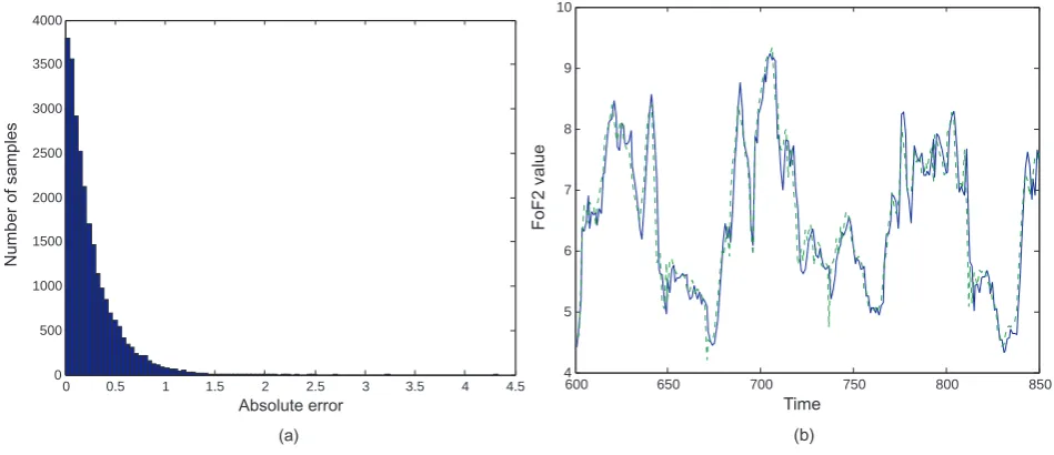
Fig. 4. One-step ahead (15 min) prediction, with the persistence predictor. (a) The histogram of the absolute differences of the computed and
the actual outputs, for the test set. (b) The actual (solid line) and the computed (dotted line) outputs for a short time interval of the test set.
24
a) ( Absolute error
Number
of
samples
b) ( Time
FoF2
value
0 0.5 1 1.5 2 2.5 3 3.5 4 4.5 0
500 1000 1500 2000 2500 3000 3500 4000
600 650 700 750 800 850
4 5 6 7 8 9 10
Figure 5:
24
a) ( Absolute error
Number
of
samples
b) ( Time
FoF2
value
0 0.5 1 1.5 2 2.5 3 3.5 4 4.5 0
500 1000 1500 2000 2500 3000 3500 4000
600 650 700 750 800 850
4 5 6 7 8 9 10
Figure 5:
Fig. 5. One-step ahead (15 min) prediction, with the 9 nearest neighbor predictor. (a) The histogram of the absolute differences of the
computed and the actual outputs, for the test set. (b) The actual (solid line) and the computed (dotted line) outputs for a short time interval of the test set.
series forecasting methods. Specifically, assuming thatn de-notes the current time slot, the purpose is to estimatex(n+1) based onx(n), . . . , x(n−(d−1)), where{x(n)}denotes the f oF2 time series. Our first concern was to estimate the value ofd, the dimension of the space where the dynamical sys-tem that generates the observedf oF2 measurements is em-bedded. This was carried out by applying the false nearest neighbor method. Then, based on the estimated value ofd, we generated the appropriate training and test sets for the training and the evaluation of the performance of four well-known predictors: the linear predictor, the two-layer,
feed-forward neural network predictor, the persistence predictor and thek-nearest neighbor predictor.
[image:7.595.60.535.328.533.2]3042 K. Koutroumbas and A. Belehaki: One-step ahead prediction off oF2 using time series forecasting techniques Below, we briefly give some future guidelines for further
investigation. First, we intend to apply nonlinearity tests on the observed data series, in order to gain some further insight on the nature of the process that produces the observedf oF2 measurements (see, e.g. Schreiber and Schmitz, 2000).
Furthermore, an interesting variation during the training of the predictor would be to supply additional information related to the presence or the absence of a disturbance.
In addition, it seems interesting to see how the above pre-dictors can be adapted in a time-varying environment. In such an environment the time series at hand exhibits signif-icant variations in time and, thus, the predictor has to adapt its parameters in order to be able to follow these changes. In this case we say that we deal with adaptive predictors. In the prediction of thef oF2, the above idea may be utilized as follows: first, we use the data of a short time period to train a specific predictor. Then, this predictor is used with the cur-rent parameter values for prediction for a short time period in the future. Then, its parameters are re-evaluated in light of the new observations and the procedure is repeated.
Finally, an obvious extension of the above work is the multi-step ahead prediction, where, of course, the error esti-mate is expected to increase, compared to that of the one-step ahead prediction. It should be noted however, that allowing the time delayT to take values other than 1, interesting re-sults may be obtained in this direction. For example, if we set T=26 (which corresponds to 6.5 h, since the sampling rate for the data set at hand is 15 min), the predictions exhibits a mean square error slightly greater than 1 MHz.
Acknowledgements. A preliminary version of this work was pre-sented in the first European Space Weather week as a contribution to the COST724 European action. Part of this work was funded by the DIAS project, sponsored by the eContent programme of the European Commission. The authors would like to thank the two reviewers for their constructive comments.
Topical Editor M. Pinnock thanks E. Tulunay and another ref-eree for their help in evaluating this paper.
References
Anderson, D. N., Buonsanto, M. J., Codrescu, M., Decker, D., Fe-sen, C. G., Fuller-Rowell, T. J., Reinisch, B. W., Richards, P. G., Roble, R. G., Schunk, R. W., and Sojka, J. J.: Intercomparison of physical models and observations of the ionosphere, J. Geophys. Res., 103, 2179–2192, 1998.
Fuller-Rowell, T. J., Codrescu, M. V., and Araujo-Pradere, E.: Cap-turing the storm-time F-region ionospheric response in an empir-ical model, AGU Geophysempir-ical Monograph, 125, 393–402, 2001. Haykin, S.: Neural Networks: A comprehensive foundation,
McMillan, 1994.
Hegger, R., Kantz, H., and Schreiber, T.: Practical implementation of nonlinear time series methods: The TISEAN package, Chaos, 9, 413–440, 1999.
Kennel, B. K., Brown, R. and Abarbanel, H. D. I.: Determining embedding dimension for phase-space reconstruction using a ge-ometrical construction, Physical Review A, 45(6), 3403–3411, 1992.
McKinnell, L. A. and Poole, A. W. V.: The development of a neural network based short term foF2 forecast program, Phys. Chem. Earth, Part C, 25(4), 287–290, 2000.
Mendenhall, W. and Sincich, T.: Statistics for engineering and the sciences, Prentice Hall, 4th edition, 1995.
Muhtarov, P. and Kutiev, I.: Autocorrelation method for temporal interpolation and short-term prediction of ionospheric data, Ra-dio Science, 34(2), 459–464, 1999.
Muhtarov, P., Kutiev, I., and Cander, L.: Geomagnetically corre-lated autoregression model for short-term prediction of ionopsh-eric parameters, Inverse Problems, 18, 49–65, 2002.
Pao, Y.-H.: Adaptive pattern recognition and neural networks, Addison-Wesley, 1989.
Rumelhart, D. E. and McClelland, J. L.: Parallel distributed pro-cessing: Explorations in the microstructure of cognition. Vol. 1: Foundations, Cambridge, MA: MIT Press, 1986.
Schreiber, T. and Schmitz, A.: Surrogate time series, Physica D, 142, 4092–4120, 2000.
Theodoridis, S. and Koutroumbas, K.: Pattern Recognition (2nd edition), Academic Press, 2003.
Tsonis, A. A.: Chaos: From theory to applications, Plenum Press, 1992.
Tulunay, Y., Tulunay, E., and Senalp, E. T.: The neural network technique – 1: a general exposition, Adv. Space Res., 33, 983– 987, 2004a.
Tulunay, Y., Tulunay, E., and Senalp, E. T.: The neural network technique – 2: an ionospheric example illustrating its application, Adv. Space Res., 33, 988–992, 2004b.