An improved low-order boundary element method for breaking surface waves

An improved low-order boundary element method for

breaking surface waves

N. Drimer, Y. Agnon

Department of Civil and Environmental Engineering, Technion, Haifa 32000, Israel

Received 21 February 2005; received in revised form 16 August 2005; accepted 27 September 2005 Available online 28 November 2005

Abstract

A new compatibility condition, applied to the velocity of the free surface particles, enables the simulation of plunging breakers, up to the creation of a thin jet, without numerical smoothing. An improved formulation of a boundary element method for the simulation of surface waves problems is derived and tested through some numerical examples. A numerical wave channel with a wavemaker and an energy absorber is developed and used for a comparison of the non-linear solution with first and second order steady solutions in the frequency domain. Finally, the shoaling of with published experimental results.

© 2005 Elsevier B.V. All rights reserved.

Keywords: Low-order boundary elements; Plunging breakers; Non-linear waves

1. Introduction

Mathematical modeling of surface waves requires the solution of a non-linear boundary value problem. One way to treat the non-linearity is by perturbation series with respect to a small parameter, usually the wave slope. However, the perturbation method is limited to weak non-linearity and cannot be used to simulate highly non-linear flows, such as wave breaking. Another approach is a fully non-linear solution by a time stepping procedure. Several numerical models have been presented in the literature, which simulate highly non-linear free surface flows, most of them are based on the boundary element method (BEM) which has the advantage of reducing the spatial dimension involved in the numerical calculations, by one.

Longuet-Higgins and Cokelet[1]presented the first numerical simulation of an overturning wave. Small instabilities, which arose in their calculations, were suppressed by a smoothing procedure. Since then, many different formulations were developed and a variety of applications were presented. Many of the models make use of complex potential or conformal mapping[1–5], hence, cannot be extended to three-dimensional problems. One formulation, which may be extended to three-dimensional problems, and is capable of accommodating a body of arbitrary shape, is the direct BEM formulation used by Jansen[6]. New et al.[7]have studied overturning waves, and their results still serve as a benchmark. A convenient method to simulate an open-ended channel is to add an artificial damping term, presented by Le Mehaute[8], to the dynamic boundary condition, in order to simulate an energy absorber. This artificial term is added only in an extension of the wave channel, hence, does not influence the solution in the physical region. Wave

∗_{Corresponding author.}

shoaling and wave breaking has been studied analytically and numerically in many studies, which are used to verify the results of the present model[9–15]. A review of most of the methods is given by Dold[2]and by Banner and Peregrine[16]. Perlin et al.[17]used particle image and tracking velocimetry in their experiments. Overturning jet velocity reached 1.7 times the linear wave theory phase velocity and the acceleration was up to 1.1 g. Chen and Kharif [18]studied breaking via the two-dimensional Navier–Stokes equation. The fluid motion was found to be irrotational up to the jet re-entry, supporting the use of a potential flow model prior to the final stage of breaking. Schaffer et al.[19]used a roller concept in a high order Boussinesq model to incorporate breaking. Grilli et al.[20]developed a fully non-linear three-dimensional model using high order BEM. Two recent reviews are presented by Grilli and Subramanya[21]and by Kim et al.[22]. Donescu and Virgin[23]have developed an Eulerian–Lagrangian implicit time integration formulation and applied it to 3D wave body interaction.

Jansen[6] discusses the order of element, which may be used in the BEM formulation, and indicates several advantages of the linear element over lower or high order elements. However, a major disadvantage of the linear element is the non-uniqueness of the normal velocity at the nodal points, which causes numerical instability when high curvature develops at the free surface. Such instability may be suppressed by smoothing but this may suppress physical instability as well. Smoothing procedures were used by Jansen as well as by many others[1,2,4,7]. While the use of high order elements is advanced and provides attractive results, it is best suited for a smooth boundary, and encounters difficulties when considering wave breaking and wave body interaction. The present work pursues an alternative course. The idea is to extend the capabilities of the simpler, linear element formulation. The linear element formulation is quite versatile, and suffers mostly from the difficulty in addressing corner flows, which arise, for example, at a breaking wave (see also Grilli et al.[20]and references therein for an evaluation of the difficulties arising at corners).

In this paper we show that the instability associated with high curvature may be removed in a physical way by defining a unique normal velocity and relating it to the element variables by means of compatibility conditions.

Following Jansen’s model, we developed an improved formulation, which enables the simulation of plunging breakers up to the creation of a very thin jet, without the use of any numerical smoothing. The angle between two adjacent normals may sometimes reach almost 180◦before the solution breaks down.

The mathematical and numerical formulations are presented in Sections2 and 3, respectively. In Sections4.1 and 4.2two verification problems of quite different nature are solved, and compared with previous results. Then the model is used to produce some new results. In Section4.3, we simulate a wave channel with a piston wavemaker and an energy absorber. A comparison of the non-linear solution with first and second order steady solutions in the frequency domain is used for the tuning of the energy absorber, and then for investigating the validity of the frequency domain models.

Several researchers utilized BEM models to investigate wave shoaling. Perhaps, the main difficulty in simulating waves shoaling is the absence of an exact mathematical expression for the radiation condition. In some works the breaker was generated by developing an initial solution of a steep sine wave, imposing periodicity conditions on both ends of the solution domain[3,6]. Such situations are useful for studying the local solution near the tip of the breaker. Recently, several works have been published, which modeled the hole shore profile, and simulate the whole shoaling process[5,9,10]. However, an initial solution of a solitary wave was used, which, as shown in the beginning of Section4.4, caused no reflection problems. The design wave used in the design of offshore and coastal structures is usually of given deep-water height and length (or period). Hence, the simulation of waves of finite length is more practical. In Section 4.4, the numerical wave channel of Section 4.3 is utilized to simulate shoaling of waves of finite length, up to breaking. The results are compared with published experimental results. The model presented here has been recently used by Song and Banner[24–26]to study the onset and strength of wave breaking in deep- and shallow-water.

2. Mathematical formulation

A two-dimensional flow in theyzplane is assumed, whereyis a horizontal coordinate along the undisturbed free surface andzis a vertical coordinate pointed upwards.

For irrotational and incompressible flow, there is a velocity potentialΦ(y,z,t) defined by

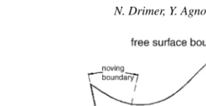
Fig. 1. Solution domain—definitions sketch. whereFis the velocity potential, satisfies Laplace’s equation:

∂2_Φ

∂y2 +

∂2_Φ

∂z2 =0 inΩ (2.2)

The solution domain,Ω, is bounded by boundaries which may be free surface, solid or artificial boundaries, as shown inFig. 1. A solid boundary may be fixed or moving. The free surface panicles satisfy the kinematic and dynamic boundary conditions:

Dx

Dt = ∇Φ, onΓf, (2.3)

DΦ

Dt = 1

2∇Φ· ∇Φ−gz, onΓf, (2.4)

wherexis the position vector (y,z) of a free surface particle andgis the gravity acceleration. The pressure above the free surface is assumed to be zero.

On a solid boundary, an impenetration boundary condition will be satisfied

∇Φ·n=Vs·n, onΓs (2.5)

wherenis a unit normal toΓ, positive out ofΩ, andVsis the local velocity of the solid boundary.

If the solution domainΩis not completely bounded by the free surfaceΓf, and the solid boundary,Γs, additional boundaries must be defined, on which boundary conditions must be formulated. Those are the artificial boundaries and some of the possible are listed below.

A simple and very popular possibility is to impose spatial periodicity, by the implementation of the boundary conditions:

Φ(0, z)=Φ(λ, z), (2.6)

∇Φ·n|(0,z)= −∇Φ·n|(λ,z), (2.7)

whereλis a pre-defined wavelength. Another possibility is to apply a linear radiation condition of the form _∂

∂t ∓Cn· ∇

Φ=0, (2.8)

on a vertical boundary.

Cis a given phase velocity and the sign∓defines a±ypropagation, respectively. The linear radiation condition is correct for a periodic wave with a known phase velocityC; but since for non-linear waves this is usually not the case; the artificial boundary will reflect some energy to the solution domain.

increasing, from the artificial boundary along the damping region. One disadvantage of the artificial damping method is the increase of computation time by adding elements. In order to absorb satisfactorily steep waves, the extension length has to be about one wavelength.

3. Numerical formulation

The initial boundary value problem is solved by a time stepping procedure, where in each time step a boundary value problem is solved in the instantaneous spatial domain. In an improved method for solving the boundary value problem is developed. The time stepping procedure is described in Section3.2.

3.1. Solution of the boundary value problem

The basis for the numerical evaluation ofΦis the familiar boundary element method. The direct formulation for a potential problem is used. According to the direct formulation a boundary integral equation is derived by the application of Green’s theorem to the velocity potentialΦand a simple source, over a closed contourΓ enclosingΩ. The resultant integral equation is:

αΦ(ξ, t)=

Γ[Φ(x, t)

∂

∂n(lnr)−lnr ∂

∂nΦ(x, t)]dΓ (3.1)

where

α=

2π, ξinΩ

Γ, ξonΓ(inner angle of the contourΓ) (3.2)

andris the distance betweenxandξ.

Then, an algebraic formulation is derived, by means of discretization of the boundaryΓ to finite elements, along which the unknown functions are approximated by their nodal values multiplying by interpolation functions (seeFig. 2):

Φ=Φ1ψ1+φ2ψ2, (3.3)

∂Φ ∂n = _∂Φ ∂n 1

ψ1+

_∂Φ

∂n

2

ψ2, (3.4)

x=x1ψ1+x2ψ2, (3.5)

where the local nodes 1 and 2 of elementjare the global nodesj,j+ 1, respectively, andψ1,ψ2are linear interpolation functions in the element region:

          

ψ1=

1 2(1−τ)

ψ1=

1 2(1−τ)

−1≤τ≤1

(3.6)

The arc length dΓ is, by definition:

dΓ =(dxdx)1/2=  

₂

k=1

ykψk 2

+

₂

k=1

zkψk 2

 1/2

dτ= 1

2Sjdτ (3.7)

whereSjis the length of the elementj, and () denotes derivative byτ.

The boundary integral in(3.1)is then approximated as a sum of integrals of the interpolation functionsψ1and

ψ2 (3.6)over the boundary elements, where the unknown values ofΦ and its gradient are left out of the integrals. Satisfying(3.1)for each of theNboundary nodes, results with a set ofNequations with 3Nunknowns

N

j=1

Aijφj−B(ij−) _∂Φ

∂n

(−) j −

B(+) ij _∂Φ ∂n (+) j

=0, i=1,2, . . . , N (3.8)

where

Aij =1 2Sj−1

ej₋1 ψ2

∂

∂n(lnr)dτ+

1 2Sj

ejψ1

∂

∂n(lnr)dτ−δijαj, (3.9)

        

B(−) ij =

1

2Sj−1

ej₋1

ψ2lnrdτ

B(+) ij =

1 2Sj

ejψ1lnrdτ

(3.10)

ris the distance between nodeiand nodejandejindicates integration along thejth element. In the geometry repre-sentation by linear elements, the unit normals,nj are constants along each element and non-continuous between the elements. Hence, care must be taken to distinguish between the unknowns

           _∂Φ ∂n (−) j = ∇

Φnj−1, x=xj _∂Φ

∂n

(+) j = ∇

Φnj, x=xj

(3.11)

The indexjshould be understood as an element index forSjandnj, and as a global node index for _∂Φ

∂n

j,Φjand

xj. The components of the unit normalnjare related to the element nodes’ location by

nj= _S1

In order to formulate a solution method which distinguish between the normal velocities, a compatibility condition relating∂Φ_∂n(_j−)and∂Φ_∂n(_j+)is required.

A tangential derivative, of any functionffollowing a free surface particle, may be computed by (finite difference central derivative)

∂f

∂s =

fj+1−fj−1

DSj , (3.13a)

DSj=

(yj+1−yj−1)2+(zj+1−zj−1)2 1/2

, (3.13b)

wherefj is the value offat the location of the jth particle. To the same degree of approximation the slope of the tangential velocity of thejth particle will be

∂y ∂z= _∂y ∂z ∂z ∂s

= yj+1−yj−1

zj+1−zj−1

. (3.14)

This is the slope of a line from nodej−1 to nodej+ l shown inFig. 2.

The true normal velocity of thejth particle is the velocity component, which is normal to the tangent defined by (3.14). Hence, the components of the truejth unit normal are

nj = 1

DSj(zj+1−zj−1, yj−1−yj+1). (3.15) Since the velocity vector of any particle is unique, the following compatibility conditions have to be satisfied

           _∂Φ ∂n (−) j =

cosβ(_j−) _∂Φ

∂n

j− sinβ(_j−)

_∂Φ ∂s j _∂Φ ∂n (+) j =

cosβ(_j+) _∂Φ

∂n

j+ sinβ(_j+)

_∂Φ

∂s

j

, (3.16)

whereβ_j(∓)is the angle betweenn_j(∓)andnjas shown inFig. 2. The tangential velocity of thejth particle is by(3.13a) _∂Φ

∂s

j=

Φj+1−Φj−1

DSj (3.17)

If the boundaryΓ is smooth at nodej(␣j=π), the compatibility condition is reduced to _∂Φ ∂n (−) j = _∂Φ ∂n (+) j = _∂Φ ∂n j . (3.18)

Hence, the normal velocity∂Φ_∂njshould not be split into∂Φ_∂nj(−),∂Φ_∂n(_j+)along the straight segments of the solid or artificial boundaries.

At the corners the free surface and the solid or artificial boundaries,∂Φ_∂njwill be split, but since at those corners two boundary conditions should be satisfied, the compatibility condition(3.16)is not needed.

Substituting the compatibility conditions for the internal free surface particles(3.16)in(3.8)we obtain

N

j=1

[AijΦj]−

j∈Γ j∈Γs

a

(B(_ij−)+B_ij(+)) _∂Φ ∂n j − jcorners

B(−) ij

_∂Φ

∂n

(−) j +

B(+) ij ∂Φ ∂n (+) j −

j∈Γ

B(n)_ij

_∂Φ

∂n

j+

B(s)_ij

_∂Φ

∂s

j

where

B_ij(n)=B(−)

ij cosB(j−)+Bij(+)cosβ(j+), (3.20)

B_ij(s)=B(−)

ij sinB(j+)+Bij(−)sinβ(j−). (3.21) Since ∂Φ_∂sj is related toΦj−1andΦj+1 by (3.17),(3.19)is a linear system of N algebraic equations with 2N unknowns. For a givenΦj or

_∂Φ ∂n

jat each nodal point (by the boundary conditions), at each time step, the system may be solved to find∂Φ_∂njorΦj, respectively.

3.2. The time stepping procedure

Similar procedures were used in previous works where the main differences are in the method of solution of the boundary value problem, the method of time integration, and the use of Lagrangian or Eulerian representation of the free surface. We use the formulation, a fourth order Runge–Kutta time integrating procedure, and the boundary value solver described in Section3.1. The time stepping procedure may be described by the following flow chart.

4. Results and discussion

First, the method is tested through some numerical examples, by comparison with previous results. In Section 4.1, the evaluation of a steep propagating wave is considered while in Section4.2a steep but steady standing wave is followed. These are two problems with quite different nature. In the first, the program is required to follow an extremely unstable wave, which breaks after about half a period. A plunging breaker with a thin jet is created which causes sharp angles between adjacent free surface elements. The standing wave is smooth, also steep, and here the program is tested to follow an exact (25th order) steady solution, during 100 periods.

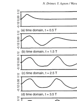
Fig. 3. Breaking of a steep sinusoidal wave. Comparing with Jansen[6]. Parameters of initial wave: wave steepnesska= 0.4084, water depth ka= 0.8168 (linear wave theory).

4.1. Breaking of steep sinusoidal wave

One very popular problem, treated by developers of methods for the evaluation of non-linear free surface flow, is the development of a plunging breaker from very steep sine wave. This situation is not very physical. However, it is proper for examining the performances of the different methods. Our results have been compared with previous simulations of overturning waves made using two different methods. The first model, presented by Jansen[6]used a method which is similar to that used for the present model, but without the new compatibility condition for the particles’ velocity. The second model, presented by New et al.[7]use an alternative numerical method. Both of the models make use of smoothing procedures to prevent numerical instabilities.

The problem is defined by Eqs.(2.2)–(2.7), and an initial solution which is a sine Stokes wave defined by a given steepnesska, and non-dimensional water depthkh, wherek,aandhare the wavenumber, wave amplitude and water depth, respectively.

Fig. 3a presents the free surface profile att= 0.38T, whereTis the linear wave period, for an initial wave parameter ka= 0.4084,kh= 0.8168. Jansen’s results, using 60 free surface particles are shown by a solid line, while results of the present model, using 90 free surface particles, are shown by dots representing particles. Shortly after this time Jansen’s calculations break down due to the high curvature at the tip of the jet. The calculations continued after a special treatment of two points at the tip of the jet, which, in addition to a smoothing procedure applied every five time steps, enabled to follow the free surface untilt= 0.46T, shown atFig. 3b. The improved method presented here enabled us to follow the free surface untilt= 0.46Twithout any definition of special points during the solution and with no use of any smoothing procedure. The improvement, formulated here, was guided by Jansen’s inspection of the instability problem, and his attempt to treat it by the special points. InTable 1, the error in energy conservation during the solution is presented for Jansen’s and for the present solution.

Fig. 4presents a solution of a similar problem which was evaluated for comparison with New et al.[7]; the parameters of the initial wave are:ka= 0.4191 andkh= 0.8375. As it may be seen, better agreement between the two models was achieved at this simulation. New et al.[7]presented the free profile att= 0.438Tand 0.477T. We present one more profile att= 0.567T, shortly before the numerical model broke down. Fifty-nine and 60 free surface particles were used by New et al.[7]and in the present simulation, respectively. The relative error in conservation of energy was 1.2%. 2.4% and 7% att= 0.438, 0.499 and 0.567, respectively.

Table 1

Error in energy conservation

t/T ET/1₄ρga2

0

Relative error [ET(t)−ET(0)]/ET(0)

Jansen Present model Jansen Present model

0.0 2.012 2.0120 0.0 0.0

0.14 2.012 2.0122 5.5×10−3 _9.9×10−5

0.28 2.033 2.0157 1.0×10−2 _1.8×10−3

0.37 2.036 2.0290 1.2×10−2 8.4×10−3

0.46 – 2.0688 – 2.8×10−2

4.2. Steep standing wave

Another verification problem is the simulation of standing wave in a rectangular basin. The model is tested to follow an “exact” solution developed by Schwartz and Whitney[11]up to 25th order in the wave steepness, for infinite water depth. The wave steepness was taken as the limit of convergence of the analytical solution,ka= 0.3. The wavelength and the basin length were set to 2π. The basin depth in the numerical model was set to 2πin order to approximate infinite depth. The free surface, basin bottom and each of the two vertical walls was divided into 32, 8 and 16 elements, respectively, i.e. 72 elements total. The time step was T0/32, where T0= 6.352456 is the period calculated by the analytical solution.

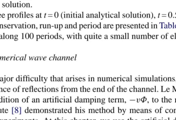
The free profiles att= 0 (initial analytical solution),t= 0.5T, 100Tand 100.5T, are presented inFig. 5. The errors in energy conservation, run-up and period are presented inTable 2. As may be seen, the numerical model keeps reasonable accuracy along 100 periods, with quite a small number of elements.

4.3. A numerical wave channel

One major difficulty that arises in numerical simulations, as well as in physical experiments, in a wave channel, is the existence of reflections from the end of the channel. Le Mehaute[8]presented a method to simulate wave absorber by the addition of an artificial damping term,−vΦ, to the right-hand side of the dynamic boundary condition(2.4). Le Mehaute[8] demonstrated his method by means of comparison between an analytical linear solution and wave channel experiments. At this chapter, we use the artificial damping term to simulate a wave absorber at the end of a

Fig. 5. Standing wave in a rectangular basin. Verification of the numerical solution’s ability to follow on analytical solution, which was developed by Schwartz and Whitney[11]up-to 25th order in the wave steepness. Parameters: unit wavenumberk= 1, basin lengthLk= 2π, basin depthhk= 2π (infinite), wave steepnessak= 0.3.

numerical wave channel. The wave channel simulator is tested to develop a solution comparable to first and second order analytical solutions to the wavemaker problem. As was indicated by Le Mehaute[8]in order to decrease the reflections caused by the wave absorber, the artificial damping coefficientvmust increase gently along the channel. After some numerical experiments we present the following example:

The channel is of unit depth (at rest)h= 1, and a total lengthL= 32. The piston wavemaker starts with harmonic motion att= 0. The piston displacement is given by

Yp=

−Ap, t≤0

−Apcos(ωt), t >0

(4.1)

whereApis the piston amplitude andωis the angular frequency.ωcorresponds to a wavelengthλ= 8, by the linear dispersion relation.

Table 2

Errors in the simulation of standing waves

Time step t/T0 No. of oscillations of the numerical solution Relative error

Period Run-up Energy

0 0.0 0 – – –

16 0.5 0.5 – – −3.0×10−4

3207 100.22 100.5 2.8×10−3 _5.0×10−3 _−2.4×10−3

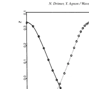
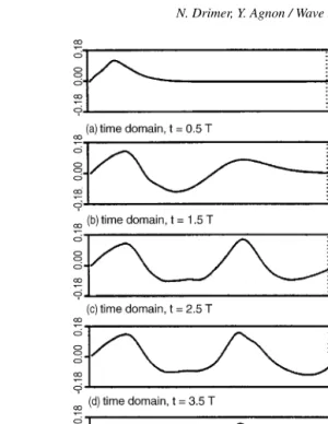
Fig. 6. A simulation of a wave channel with a piston wavemaker and an energy absorber. The development of the free surface in time, (a–e), up to a steady state, (f), which is compared to an analytical solution in the frequency domain, of second order, (g). Parameters:L/Ap/λ(linear)/h= 32/0.05/8/1.

Half of the channel,Yp<y< 16, is a physical region, while the other half, 16 <y< 32, is an energy absorbent region. The artificial damping coefficientvincreases fromv= 0, aty= 16 tov= 0.5ρωaty= 32, whereρis the fluid density. Fourfigures are presented (6, 7, 8 and 9)for four wavemaker amplitudes,Ap= 0.05, 0.1, 0.15 and 0.2, respectively. Each of the figures contains seven sub figures showing free surface profiles.

The upper five show the wave development, after the initiation of the wavemaker, atTis the wavemaker period. At the sixth sub figure, the free surface profiles at 0.5T, 1.5T, 2.5T, 3.5Tand 4.5Tare shown by a dotted line (each dot represents a particle in the numerical model), and a steady solution results of a second order analytical solution in the frequency domain, is shown by a solid line. The lowest sub figure presents first and second order analytical solutions by a dotted and a solid line, respectively. The second order solution was calculated by means of an eigenfunctions expansion, as described by Drimer and Agnon[12].

As may be seen, the solution became steady after about four periods. The waves are almost completely damped while propagating one way through the damping region. Some amount of reflection by the end may be attenuated on the way back, from the end wall to the between the physical region and the damping region.

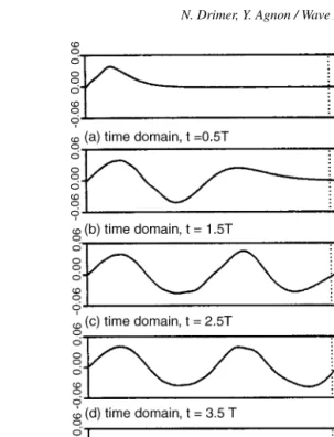
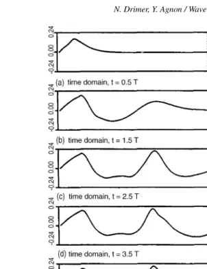
Fig. 7. A simulation of a wave channel with a piston wavemaker and an energy absorber. The development of the free surface in time, (a–e), up to a steady state, (f), which is compared to an analytical solution in the frequency domain, of second order, (g). Parameters:L/Ap/λ(linear)/h= 32/0.10/8/1.

it may be concluded that reflections from the damping region are quite small. While increasing the amplitude to 0.1, the non-linearity causes the crest to be and more pointed than the trough. Up to one wavelength away from the wavemaker the fully non-linear and the second order solution are very similar. Closer to the damping region small differences may be observed which may be caused by three reasons: some amount of reflections from the damping region, the analytical solution error by neglecting higher order terms and numerical error of the non-linear solution.

Further increasing of the wavemaker amplitude results in increasing the difference between the solutions, also good agreement is still achieved near the wavemaker.

For the largest amplitude,Ap= 0.2 (Fig. 9), a small crest develops at the center of the trough, due to the second order solution. This small crest is not confirmed by the non-linear solution and it may be cancelled by higher order terms.

The Shore Protection Manual presents a diagram by which a suitable wave theory may be chosen depending on the two parameters: _gTH2 and

h

gT2, whereHandhare the wave height and the water depth, respectively. In our example,

H

gT2 = 0.0017, 0.0033, 0.005 and 0.0067, forAp= 0.05, 0.1, 0.15 and 0.2, respectively. (Hwas calculated from the linear

transfer function of the piston wavemaker.)

Fig. 8. A simulation of a wave channel with a piston wavemaker and an energy absorber. The development of the free surface in time, (a–e), up to a steady state, (f), which is compared to an analytical solution in the frequency domain, of second order, (g). Parameters:L/Ap/λ(linear)/h= 32/0.15/8/1.

confirm the above recommendation except the possibility of using linear wave theory for the smallest amplitude (Fig. 6).

The numerical wave channel was divided into 142 elements, 80 on the free surface, 8 on the wavemaker board, 6 on the reflecting wall and 48 on the bottom. The time step wasT/32.

4.4. Wave shoaling

Fig. 9. A simulation of a wave channel with a piston wavemaker and an energy absorber. The development of the free surface in time, (a–e), up to a steady state, (f), which is compared to an analytical solution in the frequency domain, of second order, (g). Parameters:L/Ap/λ(linear)/h= 32/0.20/8/1.

The solitary wave is produced by a piston wavemaker, which processes the motion (Sugino et al.[13])

YpAptanh[Ω(t−t0)], where

Ap=0.6h0.

Ω=0.5

_g

h0

,

t0=5

h0

g,

andh0is the still water depth near the piston.

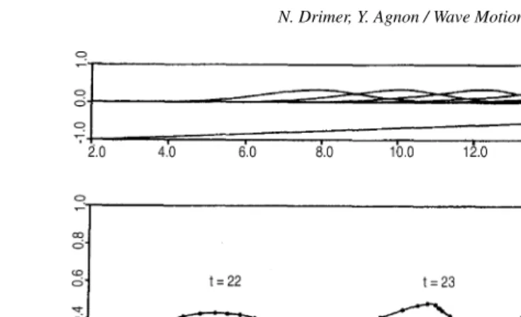
Fig. 10. Simulation of a solitary wave shoaling using a numerical wave channel. Free surface profiles at sequential times (t= 12, 14, 16, 18, 20, 21, 22, 23, 23.6, 24), until wave breaking. Units: lengthh0= 1, time (h0/g)1/2= 1.

The channel length,L= 22h0is composed of a horizontal interval of length2h0and an inclined interval of horizontal length 20h0and of slopeS= 0.04. The cannel is terminated by a reflecting wall.

Fig. 10presents successive free surface profiles up to a developed plunging breaker. The wave propagates until breaking while no significant energy is reflected by the quite close end wall.

This example also demonstrates the ability of the new formulation to follow the free surface up to the development of an angle of almost 180◦(a cusp) between elements, before a numerical instability occurs.

Since the piston is stopped, the total energy in the channel is to be conserved. The relative error in energy conservation att=24√h0/g(the last profile presented) is

E(t=24)−E(T =12)

E(t=12) =2.7×10

−3

For this example, the channel was divided into 121 elements, 80 on the free surface, 8 on the piston, 12 on the end wall, and 21 on the bottom. The time step wast= ₃₀1√h0/g.

The solitary wave is determined by two parameters wave height and water depth. Usually a design wave (in a deterministic approach) is determined by a given period and height at deep-water and its height variation versus the local depth relation is of interest. Since the design wave is one of a wave group the energy of the leading waves is to be absorbed. Numerical wave channel presented at Section4.3was used to demonstrate shoaling of a periodic wave group. The following parameters were chosen in order to compare with an experiment made by Hansen and Svendsen [14]:

deep water wave height H_∞= 37.5 mm deep water wave period T_∞=1.67 s sea bottom slope S=1 : 35

In order to reduce the time of calculations, the wave shoaling was evaluated up to a finite depthh0= 300 mm by linear wave theory according to which the wave height at depthh0isH0= 36.5 mm and the wavemaker periodT0is equalT_∞.

The wavemaker motion was

Fig. 11. Simulation of wave shoaling, using o numerical waves channel. Longitudinal cross-sections of the channel with free surface profiles, at sequential times.

wheret0is a time constant which controls the amplitude increase, which was set tot0=T0in this example. Assuming the second wave will break in the physical region, and to a linear solution of the piston wavemaker the correspondence wavemaker amplitude isAp= 0.092h0.

The wavelength ath0isλ0= 8.868, by linear theory. The numerical channel is composed of a section of uniform depthh0, of lengthλ0, a section of sloped bottom 1:35 of length 35 (h0−hmin), wherehmin= 0.21h0, and a damping region of uniform depthhminof lengthλ0. Along the damping region, the artificial damping coefficientvincreases linearly from 0 to 0.3.

Fig. 13. Wave shoaling. Wave’s height vs. water depth. Comparison among Hansen and Svendsen’s[14]experimental results, Stiassnie and Peregrine [15]theoretical results, and present model. Parameters: wave’s height at deep-water 37.5 mm, wave period 1.67 s, bench slope 1:35.

In scale longitudinal cross-sections of the channel, with free surface profiles at successive times are shown inFig. 11. The first generated wave is absorbed by the damping region, while the second wave is broken in the physical region. Fig. 12focuses on the breaker.

In Fig. 13, the wave height versus water depth curve is presented and compared to experimental and theoretical results. Results of Hansen and Svendsen’s[14]experiments were taken from Stiassnie and Peregrine[15]who used it to compare with theoretical results they developed by solving conservation equations, assuming gentle slope. Results of linear shoaling theory are also shown.

Up to depth of 200 mm an agreement exists between the numerical results, the theoretical results and the experimental results. This confirms the use we made of linear theory for transformation from deep-water to depthh0= 300 mm. At abouth= 200 mm the linear theory starts to differ from the reality while the finite amplitude theory of Stiassnie and Peregrine[15]and the present model continues to follow the experimental results. Ath= 100 mm the symmetric wave assumption of the gentle slope theory does not hold and the wave height is overestimated. The results of the present model continue to follow the experimental results almost until wave breaking. Close to breaking the calculated wave is higher than the measured wave, possibly due to neglecting of viscosity. The breaking is characterized by a prostration of the curve.

5. Conclusions

The application of a compatibility condition to the velocity of the free surface particles prevents numerical insta-bilities found in previous models, which used boundary element methods with linear elements. The source for the instabilities, as was detected by was non-uniqueness of the normal velocity at the nodal points, which breached the stability when the angle between the normals of two adjacent elements became greater than about 40◦. A definition of a unique normal at each nodal point enables the development of almost 180◦between two adjacent normals.

A new formulation, using the above compatibility condition, was derived and tested through some numerical examples.

An artificial damping term, which is added to the dynamic free surface boundary condition, may be used for the simulation of an energy absorber at the end of a numerical wave channel. This is demonstrated by comparison of the non-linear solution with first and second order solutions of the piston wavemaker problem.

Potential theory gives reasonable results for wave shoaling up to breaking. The use of an artificial energy absorber enables the simulation of shoaling of a periodic wave in a quite practical situation. This is demonstrated by a comparison of numerical results with published experimental results.

References

[2] J.W. Dold, An efficient surface-integral algorithm applied to unsteady gravity waves, J. Comp. Phys. 103 (1) (1992) 90–115. [3] T. Vinje, P. Brevig, Numerical simulation of breaking waves, Adv. Water Resour. 4 (1981) 77–82.

[4] J.W. Dold, D.H. Peregrine, An efficient boundary integral method for steep unsteady water waves, Numer. Methods Fluid Dyn. II (1986) 671–679.

[5] M.J. Cooker, A boundary-integral method for water wave motion over irregular beds, Eng. Anal. Boundary Elements 7 (4) (1990) 205–213. [6] P.C.M. Jansen, A Boundary Element Model for Non-Linear Free Surface Phenomena, Delft University of Technology, Report No. 86-2, 1986. [7] A.L. New, P. McIver, D.H. Peregrine, Computations of overturning waves, J. Fluid Mech. 150 (1985) 233–251.

[8] B. Le Mehaute, Progressive wave absorber, J. Hydraulic Res. 10 (2) (1972) 153–169.

[9] A.K. Otta, I.A. Svendsen, S.T. Grilli, The breaking and run-up of solitary waves on beaches, Coastal Eng. 112 (1992) 1461–1474. [10] J. Broeze, Computation of breaking waves with a panel method, J. Fluid Mech. 190 (1992) 141–163.

[11] L.W. Schwartz, A.K. Whitney, A semi-analytic solution for non-linear standing waves in deep water, J. Fluid Mech. 107 (1981) 147–171. [12] N. Drimer, Y. Agnon, A hybrid boundary element method for second-order wave–body interaction, Appl. Ocean Res. 16 (1994) 27–45. [13] R. Sugino, H. Kawabata, N. Tosaka, Nonlinear free surface flow problems by boundary element—Lagrangian solution procedure, in: Boundary

Element Methods, Pergamon Press, 1990.

[14] J.B. Hansen, I.A. Svendsen, Regular waves in shoaling water experimental data, Institute of Hydrodynamics and Hydraulic Engineering Technology, University of Denmark, Series Paper No. 21, 1979.

[15] M. Stiassnie, D.H. Peregrine, Shoaling of finite-amplitude surface waves on water of slowly varying depth, J. Fluid Mech. 97 (1980) 783–805. [16] M.L. Banner, D.H. Peregrine, Wave breaking in deep water, Ann. Rev. Fluid Mech. 25 (1993) 373–397.

[17] M. Perlin, J. He, L.P. Bernal, An experimental study of deep water plunging breakers, Phys. Fluids 8 (9) (1996) 2365–2374. [18] G. Chen, C. Kharif, Two-dimensional Navier–Stokes simulation of breaking waves, Phys. Fluids 11 (1) (1999) 121–133.

[19] H.A. Schaffer, P.A. Madsen, R. Deigaard, A Boussinesq model for waves breaking in shallow water, Coastal Eng. 20 (1993) 185–202. [20] S.T. Grilli, P. Guyenne, F. Dias, A fully non-linear model for three-dimensional overturning waves over an arbitrary bottom, Int. J. Num.

Methods Fluids 35 (7) (2001) 829–867.

[21] S.T. Grilli, R. Subramanya, Recent advances in the BEM modelling of nonlinear water waves, in: H. Power (Ed.), Boundary Element Applications in Fluid Mechanics, Advances in Fluid Mechanics Series, Computational Mechanics Publication, Southampton, UK, 1995, Chapter 4, pp. 91–122.

[22] C.H. Kim, A.H. Clement, K. Tanizawa, Recent research and development of numerical wave tank—a review, Int. J. Offshore Polar Eng. 9 (4) (1999) 241–256.

[23] P. Donescu, L.N. Virgin, An implicit boundary element solution with consistent linearization for free surface flows and non-linear fluid–structure interaction of floating bodies, Int. J. Num. Methods Eng. 5 (4) (2001) 379–412.

[24] J.-B. Song, M.L. Banner, On determining the onset and strength of breaking for deep water waves. Part I: unforced irrotational wave groups, J. Phys. Oceanogr. 32 (9) (2002) 2541–2558.

[25] M.L. Banner, J.-B. Song, On determining the onset and strength of breaking for deep water waves. Part II: influence of wind forcing and surface shear, J. Phys. Oceanogr. 32 (9) (2002) 2559–2570.