Fractional baud-length coding

(1)

Ann. Geophys., 29, 1189–1196, 2011 www.ann-geophys.net/29/1189/2011/ doi:10.5194/angeo-29-1189-2011

Annales

Geophysicae

Fractional baud-length coding

J. Vierinen

Sodankyl¨a Geophysical Observatory, Sodankyl¨a, Finland

Received: 24 March 2010 – Revised: 8 February 2011 – Accepted: 6 June 2011 – Published: 30 June 2011

Abstract. We present a novel approach for modulating radar transmissions in order to improve target range and Doppler estimation accuracy. This is achieved by using non-uniform baud lengths. With this method it is possible to increase sub-baud range-resolution of phase coded radar measurements while maintaining a narrow transmission bandwidth. We first derive target backscatter amplitude estimation error covari-ance matrix for arbitrary targets when estimating backscatter in amplitude domain. We define target optimality and dis-cuss different search strategies that can be used to find well performing transmission envelopes. We give several simu-lated examples of the method showing that fractional baud-length coding results in smaller estimation errors than con-ventional uniform baud length transmission codes when es-timating the target backscatter amplitude at sub-baud range resolution. We also demonstrate the method in practice by analyzing the range resolved power of a low-altitude meteor trail echo that was measured using a fractional baud-length experiment with the EISCAT UHF system.

Keywords. Radio science (Ionospheric physics; Signal pro-cessing; Instruments and techniques)

1 Introduction

We have previously described a method for estimating range and Doppler spread radar targets in amplitude domain at sub baud-length range-resolution using linear statistical inversion (Vierinen et al., 2008b). However, we did not use codes opti-mized for the targets that we analyzed. Also, we only briefly discussed code optimality. In this paper we will focus on optimal transmission codes for a target range resolution that is smaller than the minimum allowed baud-length. We will introduce a variant of phase coding called “fractional baud-length codes” that are useful for amplitude domain inversion

Correspondence to: J. Vierinen ([email protected])

of range and possibly Doppler spread targets, when a bet-ter resolution than the minimum allowed radar transmission envelope baud-length is required.

The method introduced in this study differs from the Frequency Domain Interferometry (FDI) (Kudeki and Stitt, 1987) method as it does not require the target scattering to originate from a very narrow layer within the radar scattering volume. Assuming that the target is indeed a narrow enough layer, the FDI method will probably perform better in terms of range resolution. However, it is feasible to combine frac-tional baud-length coding with FDI to obtain a shorter de-coded pulse before the interferometry step.

In radar systems there is a limit to the smallest baud length, which arises from available bandwidth due to transmission system or licensing constraints. However, the transmission envelope can be timed with much higher precision than the minimum baud length. For example, the EISCAT UHF and VHF mainland systems in Tromsø are currently capable of timing the transmission envelope at 0.1 µs resolution, but the minimum allowed baud length is 1 µs. Thus, it is possible to use transmission codes with non-uniform baud-lengths that are timed with 0.1 µs accuracy, as long as the shortest baud is not smaller than 1 µs. This principle can then be used to achieve high resolution (<1 µs) backscatter estimates with smaller variance than what would be obtained using a uni-form baud-length radar transmission code with baud lengths that are integer multiples of 1 µs.

(2)

1190 J. Vierinen: Fractional baud-length coding 2 Fractional baud-length code

We will treat the problem in discrete time. The measurement sample rate is assumed to be the same as the required target range resolution.

A transmission envelope can be described as a baseband sequence of L samples. If the transmission envelope has much less bauds NbL than samples, it is economical to represent the transmission code in terms of bauds. In this case, the envelope can be described in terms of the lengthslk∈0⊂N, phasesφk∈P⊂ [0,2π )and amplitudes

ak∈3⊂ [0,1] ⊂Rof the bauds. We can define an arbitrary transmission envelope as

t=

Nb X

j=1

[t∈Bj]ajeiφj, (1)

where[·]is the so called Iverson bracket, which evaluates to 1 if the logical expression is true – in this case when the index “t” is within the set of indicesBj= {1+Pj

−1

i=0li,2+ Pj−1

i=0li,···,lj+ Pj−1

i=0li}within baudj and zero otherwise (additionally, we definel0=0). In this study, the code power is always normalized to unityP∞

t=−∞|t|2=1, which means

that the variances are comparable between transmission en-velopes that deliver a similar amount of radar power. The codes can also be normalized otherwise, if comparison be-tween two envelopes of different total power is needed.

The transmission waveform definition is intentionally as general as possible. Radar specific constraints can be im-posed by defining the sets0, P, and3. These will be dis-cussed later on in Sect. 5.

3 Target estimation variance

The presentation here slightly differs from Vierinen et al. (2008b). Instead of a Fourier series, we will use B-splines to model the target backscatter.

Using discrete time and range, and assuming that our re-ceiver impulse response is sufficiently close to a boxcar func-tion that is matched to the sample rate, the direct theory for a signal measured from a radar receiver can be expressed as a sum of the range lagged transmission envelope multiplied by the target backscatter amplitude

mt=

X

r∈R

t−rζr,t+ξt. (2)

Heremt∈C is the measured baseband raw voltage signal,

R= {Rmin,...,Rmax} ⊂Nis the target range extent,t∈Cis the transmission modulation envelope,ζr,t∈Cis the range and time dependent target scattering coefficient andξt∈Cis measurement noise consisting of thermal noise and sky-noise from cosmic radio sources. The measurement noise is as-sumed to be a zero mean complex Gausian white noise with variance Eξtξt0=δ_t,t0σ2. Rangesrare defined in round-trip

2 J. Vierinen et al.: Fractional baud-length coding

2 Fractional baud-length code

We will treat the problem in discrete time. The measurement sample rate is assumed to be the same as the required target range resolution.

A transmission envelope can be described as a baseband sequence of L samples. If the transmission envelope has much less bauds Nb L than samples, it is economical to represent the transmission code in terms of bauds. In this case, the envelope can be described in terms of the lengths

lk ∈ Γ ⊂ N, phasesφk ∈ P ⊂ [0,2π) and amplitudes ak ∈ Λ ⊂[0,1] ⊂Rof the bauds. We can define an arbi-trary transmission envelope as

t= Nb

X

j=1

[t∈Bj]ajeiφj, (1)

where [·] is the so called Iverson bracket, which evaluates to1if the logical expression is true – in this case when the indextis within the set of indicesBj ={1 +Pj−1

i=0li,2 +

Pj−1

i=0li,· · ·, lj+P j−1

i=0li}within baudjand zero otherwise

(additionally, we definel0= 0). In this study, the code power

is always normalized to unity P∞

t=−∞|t|2 = 1, which means that the variances are comparable between transmis-sion envelopes that deliver a similar amount of radar power. The codes can also be normalized otherwise, if comparison between two envelopes of different total power is needed.

The transmission waveform definition is intentionally as general as possible. Radar specific constraints can be im-posed by defining the setsΓ,P, andΛ. These will be dis-cussed later on in section 5.

3 Target estimation variance

The presentation here slightly differs from (Vierinen et al., 2008b). Instead of a Fourier series, we will use B-splines to model the target backscatter.

Using discrete time and range, and assuming that our re-ceiver impulse response is sufficiently close to a boxcar func-tion that is matched to the sample rate, the direct theory for a signal measured from a radar receiver can be expressed as a sum of the range lagged transmission envelope multiplied by the target backscatter amplitude

mt=X r∈R

t−rζr,t+ξt. (2)

[image:2.595.312.546.64.175.2]

Here mt ∈ C is the measured baseband raw voltage sig-nal,R ={Rmin, ..., Rmax} ⊂ Nis the target range extent, t ∈ Cis the transmission modulation envelope, ζr,t ∈ C is the range and time dependent target scattering coefficient andξt∈Cis measurement noise consisting of thermal noise and sky-noise from cosmic radio sources. The measurement noise is assumed to be a zero mean complex Gausian white noise with varianceEξtξt0 =δt,t0σ2. Rangesrare defined

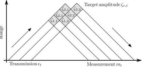
Fig. 1.Simplified range-time diagram of backscatter from a strong narrow region (notice that this is not in round-trip time). In this example there are two transmit samples and three ranges that cause backscatter. The gray area represents the area where the backscatter of one sample originates from, assuming boxcar impulse response. A longer impulse response will cause more range spreading.

in round-trip time at one sample intervals,talso denotes time in samples. By convention, we apply a range dependent con-stant₂rdelay, so that the range dependent backscatter ampli-tude isζr,tinstead ofζr,t−r

2. Fig. 1 depicts backscatter from three range gates probed with two transmission samples. To simplify matters, we use overlapping triangular range gates.

3.1 Coherent target

Now if the target backscatter is constantζr,t =ζr, the mea-surement equation becomes a convolution equation

mt =X r∈R

t−rζr+ξt, (3)

which is the most common measurement equation for radar targets. Assuming that the target is sufficiently extended, this can be solved by filtering the measurements with a filter that corresponds to the frequency domain inverse of the transmis-sion envelope (Sulzer, 1989;Ruprecht, 1989). However, for a finite range extent, the filtering approach is not always op-timal as it does not properly take into account edge effects, such measurements missing due to ground clutter or receiver protection. A sufficiently narrow range extent also results in smaller estimation errors. In these cases, one should use a linear theory matrix that explicitely defines the finite range extent. We will define this as a special case of the incoherent backscatter theory presented next.

3.2 Incoherent target

If the target backscatter is not constant, the range dependent backscatterζr,t has to be modeled in some way in order to

make the estimation problem solvable. One natural choice is to assume that the target backscatter is a band-limited sig-nal, which can be modeled using a B-spline (de Boor, 1978). Our model parameters will consist ofNscontrol points that

Fig. 1. Simplified range-time diagram of backscatter from a strong

narrow region (notice that this is not in round-trip time). In this example there are two transmit samples and three ranges that cause backscatter. The gray area represents the area where the backscatter of one sample originates from, assuming boxcar impulse response. A longer impulse response will cause more range spreading.

time at one sample intervals,t also denotes time in samples. By convention, we apply a range dependent constant r₂ de-lay, so that the range dependent backscatter amplitude isζr,t

instead ofζ_r,t−₂r. Figure 1 depicts backscatter from three

range gates probed with two transmission samples. To sim-plify matters, we use overlapping triangular range gates. 3.1 Coherent target

Now if the target backscatter is constantζr,t=ζr, the

mea-surement equation becomes a convolution equation

mt=

X

r∈R

t−rζr+ξt, (3)

which is the most common measurement equation for radar targets. Assuming that the target is sufficiently extended, this can be solved by filtering the measurements with a filter that corresponds to the frequency domain inverse of the transmis-sion envelope (Sulzer, 1989; Ruprecht, 1989). However, for a finite range extent, the filtering approach is not always op-timal as it does not properly take into account edge effects, such measurements missing due to ground clutter or receiver protection. A sufficiently narrow range extent also results in smaller estimation errors. In these cases, one should use a linear theory matrix that explicitely defines the finite range extent. We will define this as a special case of the incoherent backscatter theory presented next.

3.2 Incoherent target

If the target backscatter is not constant, the range dependent backscatterζr,t has to be modeled in some way in order to

make the estimation problem solvable. One natural choice is to assume that the target backscatter is a band-limited sig-nal, which can be modeled using a B-spline (de Boor, 1978). Our model parameters will consist ofNs control points that model the backscatter at each range of interest. The fre-quency domain characteristics are defined by the spacing of

(3)

J. Vierinen: Fractional baud-length coding 1191 the knots and the order of the splinen. Using the definition

of B-splines, the target backscatterζr,t is modeled using the

parametersPr,k∈Cas:

ˆ

ζr,t= Ns−1

X

k=0

Pr,kbk,n

_t₋₁

L−1

, (4)

wherebk,n(·)is the B-spline basis function and coefficients

Pr,k are the control points withk∈ {1,...,Ns}. We assume that the control points are evenly spaced and that the end-points contain multiple knots in order to ensure that the sec-ond order derivatives are zero at both ends ofζˆr,t. We also

define a special case of one spline control point asζˆr,t=Pr=

ζr. This corresponds to a completely coherent target.

When Eq. (4) is substituted into Eq. (2), we get

mt=

X

r∈R Ns−1

X

k=0

Pr,kt−rbk,n

_t₋₁

L−1

+ξt. (5)

This model is linear in respect to the parametersPr,kand one

can conveniently represent it in matrix form as

m=Ax+ξ, (6)

wherem= [m1,...,mN]T is the measurement vector, A is

the theory matrix containing the t−rbk,n(·) terms, x=

[P1,1,P1,2,...,PNr,Ns]

T _{is the parameter vector containing} the control points andξ= [ξ1,...,ξN]Tis the error vector with

the second moment defined as

Eξ ξH=6=diag(σ2,...,σ2). (7)

The number of parameters is the number of rangesNrtimes the number of B-spline control points Ns per range. The number of measurementsN=Nr+L−1 is a sum of target ranges and transmission envelope lengthL. As long asN≥

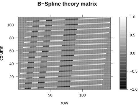
NrNsand the theory matrix has sufficient rank, the problem can be solved using statistical linear inversion. In practice, the number of model parameters that can be succesfully mod-eled with sufficiently small error bars depends on the signal to noise ratio. The estimation of strong range and Doppler spread echos is shown in Vierinen et al. (2008b). Figure 2 shows an example theory matrix for a target range extent

Nr=14 withNs=8 spline guide points per range. The trans-mission code is a uniform baud-length 13-bit Barker code with baud lengthlj=10.

The probability density for Eq. (6) can be written as:

p(m|x)∝exp

− 1

σ2km−Axk

2 ₍₈₎

and assuming constant valued priors, the maximum a poste-riori (MAP) estimate, i.e., the peak ofp(m|x)is

xMAP=(AHA)−1AHm (9)

and the a posteriori covariance is:

6p=σ2(AHA)−1. (10)

J. Vierinen et al.: Fractional baud-length coding 3

model the backscatter at each range of interest. The fre-quency domain characteristics are defined by the spacing of the knots and the order of the splinen. Using the definition of B-splines, the target backscatterζr,tis modeled using the

parametersPr,k∈Cas:

ˆ

ζr,t=

Ns−1 X

k=0

Pr,kbk,n

t−1

L−1

, (4)

wherebk,n(·)is the B-spline basis function and coefficients Pr,k are the control points with k ∈ {1, ..., Ns}. We

as-sume that the control points are evenly spaced and that the end-points contain multiple knots in order to ensure that the second order derivatives are zero at both ends of ζr,tˆ . We also define a special case of one spline control point as

ˆ

ζr,t = Pr = ζr. This corresponds to a completely coherent

target.

When equation 4 is substituted into equation 2, we get

mt= X

r∈R Ns−1

X

k=0

Pr,kt−rbk,n

t−1

L−1

+ξt. (5)

This model is linear in respect to the parametersPr,kand one can conveniently represent it in matrix form as

m=Ax+ξ, (6)

where m = [m1, ..., mN]T is the measurement vector, A

is the theory matrix containing the t−rbk,n(·) terms,x =

[P1,1, P1,2, ..., PNr,Ns]T is the parameter vector containing

the control points andξ = [ξ1, ..., ξN]T is the error vector

with the second moment defined as

EξξH=Σ= diag(σ2, ..., σ2). (7)

The number of parameters is the number of ranges Nr

times the number of B-spline control points Ns per range. The number of measurementsN =Nr+L−1is a sum of target ranges and transmission envelope lengthL. As long asN ≥NrNsand the theory matrix has sufficient rank, the

[image:3.595.309.549.61.244.2]

problem can be solved using statistical linear inversion. In practice, the number of model parameters that can be succes-fully modeled with sufficiently small error bars depends on the signal to noise ratio. The estimation of strong range and Doppler spread echos is shown in Vierinen et al. (2008b). Fig. 2 shows an example theory matrix for a target range ex-tentNr= 14withNs= 8spline guide points per range. The

transmission code is a uniform baud-length 13-bit Barker code with baud lengthlj = 10.

The probability density for Eq. 6 can be written as:

p(m|x)∝exp

− 1

σ2km−Axk 2

(8)

and assuming constant valued priors, the maximuma poste-riori(MAP) estimate, i.e., the peak ofp(m|x)is

B−Spline theory matrix

row

column

20 40 60 80 100

50 100

[image:3.595.308.508.439.476.2]

−1.0 −0.5 0.0 0.5 1.0

Fig. 2. A theory matrix for a range and Doppler spread target with

Nr = 14range gates andNs = 8B-spline guide points per range. The code is a simple 13-bit Barker code with 10 samples per baud.

and thea posterioricovariance is:

Σp=σ2(AHA)−1. (10)

3.3 Infinitely extended coherent target

In the special case of an infinitely extended coherent tar-get (Ns = 1), the matrixAbecomes a convolution opera-tor and the problem can be efficiently solved in frequency domain and numerically evaluated using FFT (Cooley and Tukey, 1965). This case has been extensively discussed by, e.g.,Lehtinen et al.(2008a);Vierinen et al.(2006);Lehtinen et al. (2004) and Ruprecht (1989). The covariance matrix will be an infinitely extended Toeplitz matrix with rows1:

Σt= lim M→∞

1

MF

−1 M

 

 FM

( _∞ X

τ=−∞

ττ−t

)!−1 

 .

This result is also a fairly good approximation for a suffi-ciently long finite range extent, differing only near the edges. However, this result is not valid for a sufficiently narrow fi-nite range extent or when the target also has Doppler spread. Also, it is not even possible to calculate the covariance matrix in this way for uniform length codes when the baud-length is larger than the target resolution. The reason for this is that for an infinitely extended target there will be zeros in the frequency domain representation of the transmission envelope and because of this, the covariance matrix is singu-lar. Even in the case of a finite range extent, all codes with

1

the indextrefers to the column of the matrix row. Operators FM and FM−1 are the forward and reverse discrete Fourier

trans-forms of lengthM. In practice the covariance can be approximated

Fig. 2. A theory matrix for a range and Doppler spread target with

Nr=14 range gates andNs=8 B-spline guide points per range.

The code is a simple 13-bit Barker code with 10 samples per baud.

3.3 Infinitely extended coherent target

In the special case of an infinitely extended coherent target (Ns=1), the matrix A becomes a convolution operator and the problem can be efficiently solved in frequency domain and numerically evaluated using FFT (Cooley and Tukey, 1965). This case has been extensively discussed by, e.g., Lehtinen et al. (2008); Vierinen et al. (2006); Lehtinen et al. (2004) and Ruprecht (1989). The covariance matrix will be an infinitely extended Toeplitz matrix with rows1:

6t= lim

M→∞

1

MF

−1

M

 

 FM

( _∞

X

τ=−∞

ττ−t

)!−1 



.

This result is also a fairly good approximation for a suffi-ciently long finite range extent, differing only near the edges. However, this result is not valid for a sufficiently narrow fi-nite range extent or when the target also has Doppler spread. Also, it is not even possible to calculate the covariance matrix in this way for uniform length codes when the baud-length is larger than the target resolution. The reason for this is that for an infinitely extended target there will be zeros in the frequency domain representation of the transmission envelope and because of this, the covariance matrix is singu-lar. Even in the case of a finite range extent, all codes with uniform baud-length result in a theory matrix with strong lin-early dependent components. An example of this is shown in Sect. 6. When using non-uniform baud-lengths the problem can be avoided, since in this way it is possible to form a code

1_{The index}_t_{refers to the column of the matrix row. Operators}

FM andF_M−1are the forward and reverse discrete Fourier

trans-forms of lengthM. In practice the covariance can be approximated

(4)

1192 J. Vierinen: Fractional baud-length coding without zeros in the frequency domain. This is somehwhat

similar to random alias-free sampling (Shapiro and Silver-man, 1960). Another analogy can be found in the use of ape-riodic radar interpulse periods to overcome range-Doppler ambiguities, e.g., (Farley, 1972; Uppala and Sahr, 1994; Pirt-til¨a and Lehtinen, 1999).

4 Code optimality

The performance of a certain code is determined by the tar-get parameter estimation errors. These on the other hand are determined by the a posteriori covariance matrix in Eq. (10). Because we assume uniform priors, the covariance matrix is fully determined by the target model (i.e., assumed target characteristics) in theory matrix A. The theory matrix A con-tains the transmission envelope and therefore it affects the covariance matrix. The task of code optimization is to find a covariance matrix that produces the best possible estimates of the target.

In terms of the theory of comparison of measurements (Pi-iroinen, 2005), a code1is in every situation better than some other code2only if the difference of their corresponding co-variance matrices62−61is positive definite. Even though it might be feasible use this as a criterion in a code search, we chose a more pragmatic approach where we construct a function that maps the the covariance matrix to a real number

:_RNp×Np_→

Rwhile still retaining some of the informa-tion contained in the covariance matrix. One such map is the trace of the covariance matrix(6)=tr(6), which is called A-optimality in terms of optimal statistical experiment de-sign. This has the effect of minimizing the average variance of the model parameters. We will use this criterion through-out this paper. Refer to, e.g., Pukelsheim (1993) for more discussion on optimization criteria.

For infinitely extended fully coherent targets, the trace of the covariance matrix is infinite, but one can use the diagonal value of one row of the covariance matrix. Because it is of Toeplitz form, all diagonal values are the same, and this will correspond to A-optimality.

5 Code search

The transmission envelope consisting ofNb bauds is fully described by the baud lengthslk∈0⊂N, phases φk∈P⊂

[0,2π )and amplitudesak∈3⊂ [0,1] ⊂R. These form the set of parameters to optimize

(lk,φk,ak)⊂0Nb×PNb×3Nb. (11)

In addition to this, the number of baudsNbin a code of length

L need not be fixed, as this depends on the lengths of the individual baudslk.

For reasonably short codes with sufficiently small num-ber of phases it might be possible to perform an exhaustive

J. Vierinen et al.: Fractional baud-length coding 5

Randomize code

Split random

baud

Change random baud length

Change random baud phase

Yes

Accept change Save

result changeReject

No

Yes

Code improved?

No

Number of iterations reached?

1 2

4

Random {1,2,3,4}

Remove random

baud

[image:4.595.354.501.55.284.2]

3

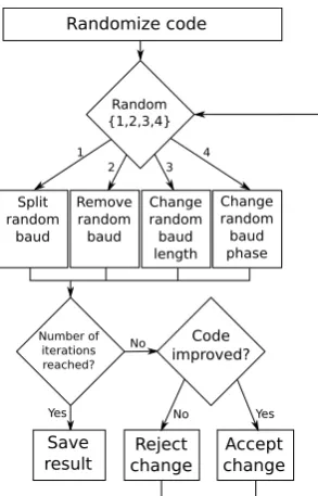
Fig. 3.Simplified block diagram of the optimization algorithm.

3. Change the length of a baud. Increase the length of one randomly selected baud and decrease the length of an-other randomly selected baud to maintain code length.

4. Change random baud phase and amplitude. Select an arbitrary baud and slightly change phase and amplitude.

These incremental changes are designed in a way that they always conform to the criteria imposed on the transmission code. If this is not possible (i.e., if it is not possible to add a new baud), the code remains unchanged. The imple-mentation ofslight changedepends on the constrains placed on the code. E.g., in the case of binary phase codes with constant amplitude, a 180◦ phase flip would correspond to a slight phase change, while the amplitudes would remain unchanged. For a polyphase code, the slight change in phase could be a small random change in the original phase

φ0_k=φk+φ, whereφwould be a small random number.

In order to initially randomize a code, we start with any phase code that conforms with the constraints of baud lengths, phases and amplitudes. This can be hard coded. We then perform a certain number of the same incremen-tal changes that we use in the optimization procedure, except that we accept all of the changes.

6 Example: Range spread coherent target

To demonstrate the performance of non-uniform baud-length codes when estimating a target at sub-baud resolution, we

simulatedan echo using a constant amplitude binary phase non-uniform length code and traditional uniform baud-length constant amplitude binary phase code of the same

length. In this example, we analyze a 10 sample wide target at the resolution of one sample. The non-uniform baud-length code was an optimized 11-bit code with baud lengths{12,12,12,12,10,13,10,11,11,15,12}and phases

{1,−1,1,−1,1,−1,1,−1,1,−1,−1}. The smallest al-lowed baud-length was10samples. For comparison we used the well known13-bit Barker code with a baud-length of10

samples. Both simulations had the same instance of mea-surement noiseSNR = 3 and the same target amplitudes, which in this case was an instance of the complex Gaussian randomN_C(0,1)process.

The results are shown in figure 4. It is evident that the non-uniform baud-length code performs better in terms of estimation errors. It is also evident that the Barker code suf-fers from the fact that every baud is the same length – if the range extent would have been infinite, the covariance matrix would have been singular. Now the covariance matrix is only near-singular. This is seen as large off-diagonal stripes in the 13-bit Barker code covariance matrix and correlated errors. In the case of the 11-bit fractional code the off-diagonal ele-ments are more uniform and the variance is also smaller.

7 Example: meteor echo structure

During the 15-19.11.2009 Leonid meteor campaign, we used a set of 53 optimized fractional baud-length codes with 0.5

µs fractional resolution and 5µs minimum baud length. The transmission pulse length was 371 µs. The data was sam-pled at samsam-pled at 2 MHz sample rate. The large number of pulses, together with the fairly long baud-length allowed simultaneous analysis of space debris and the ionosphere, while not sacrificing too much in terms of meteor head echo parameter estimation accuracy. We used the EISCAT UHF radar located in Tromso, with the 32 m antenna beam pointed approximately 99 km above Peera, Finland, giving a zenith angle of about 42◦. The radar peak power was approximately 1.4 MW.

During this campaign, one of the observed “strange” me-teor echos was an echo at approximately 60 km. The meme-teor head (or the dense cloud of plasma) is first seen decelerat-ing from about 1 km/s to 0 km/s. After this, several disjoint trail-like structures persist for nearly 2 seconds.

The meteor head echo was detected by searching for the maximum likelihood parameters for a single echo moving point-target model

mt =σt−R0exp{iωt}+ξt, (12)

whereσis the backscatter amplitude,ωis the Doppler shift and R0 is range (ξt denotes receiver noise). The

maxi-mum likelihood parameters were obtained using a grid search of the likelihood function resulting from the measurement model. This is necessary as the Doppler shift is usually sig-nificant for meteor head echos at 929 MHz with such a long pulse.

Fig. 3. Simplified block diagram of the optimization algorithm.

search. This consists of first determining all the different ways to divide a code of lengthL into bauds of lengthslk.

After this, all unique orderings of the baud-lengths and per-mutations of phases and amplitudes need to be traversed. The problem of determining the different combinations of baud lengths amounts to the problem of generating all integer par-titions forL (Kelleher and O’Sullivan, 2009). When addi-tional constraints to baud lengths are applied, the problem is called the multiply restricted integer partitioning problem (Riha and James, 1976). An efficient algorithm for iterating through restricted partitions has been described by Riha and James (1976).

The exhaustive approach fails already for reasonably small problems due to the catastrophic growth of the search space. Therefore we have to resort to some optimization method in order to find optimal codes. Optimization methods have been previously used for code searches at least by Sahr and Grannan (1993), and Nikoukar (2010). Our approach for finding optimal codes is based on the simulated annealing method (Kirkpatrick et al., 1983).

The optimization procedure that we have developed can be used to find well performing non-uniform baud-length codes, given a set of constraints. The constraints are given as the set of allowed baud lengths0, the set of allowed phases P and the set of allowed amplitudes3. We have previously used a similar algorithm to optimize codes for infinitely extented coherent targets and lag-profile inversion of incoherent scat-ter radar (Vierinen et al., 2006, 2008a).

The main principle of the algorithm is very simple. We first randomize a code E0≡(lk,φk,ak,Nb)that meets the given constraints. Next, for a certain number of iterations we incrementally attempt to improve this code with small

(5)

J. Vierinen: Fractional baud-length coding 1193 random changesE0=δEi. Hereδis an operator that slightly

modifiesEin some way, while conforming to the constraints imposed on the code. If any of these changes results in a code that is better, we then save these parametersEi+1=E0 and continue to the next iteration. In order to reduce the chance of the algorithm from getting stuck in a local minima, we also sometimes (by a small random chance) allow changes that do not improve the code. In order to achieve convergence, the magnitude of the random changesδEis decreased as the iteration advances. The algorithm is depicted in Fig. 3. The small incremental changes that we use are:

1. Split random baud. Select a long enough baud in the code and split it into two bauds. Retain the original am-plitude and phase on one of these bauds and slightly randomly modify them on the other baud.

2. Remove a random baud. Increase a randomly selected baud length.

3. Change the length of a baud. Increase the length of one randomly selected baud and decrease the length of an-other randomly selected baud to maintain code length. 4. Change random baud phase and amplitude. Select an

arbitrary baud and slightly change phase and amplitude. These incremental changes are designed in a way that they always conform to the criteria imposed on the transmission code. If this is not possible (i.e., if it is not possible to add a new baud), the code remains unchanged. The im-plementation of “slight change” depends on the constrains placed on the code. E.g., in the case of binary phase codes with constant amplitude, a 180◦_{phase flip would correspond}

to a slight phase change, while the amplitudes would re-main unchanged. For a polyphase code, the slight change in phase could be a small random change in the original phase

φ_k0=φk+φ, whereφwould be a small random number.

In order to initially randomize a code, we start with any phase code that conforms with the constraints of baud lengths, phases and amplitudes. This can be hard coded. We then perform a certain number of the same incremen-tal changes that we use in the optimization procedure, except that we accept all of the changes.

6 Example: range spread coherent target

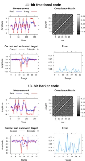
To demonstrate the performance of non-uniform baud-length codes when estimating a target at sub-baud resolution, we simulated an echo using a constant amplitude binary phase non-uniform length code and traditional uniform baud-length constant amplitude binary phase code of the same length. In this example, we analyze a 10 sample wide target at the resolution of one sample. The non-uniform baud-length code was an optimized 11-bit code with baud lengths {12,12,12,12,10,13,10,11,11,15,12} and phases

{1,−1,1,−1,1,−1,1,−1,1,−1,−1}. The smallest allowed baud-length was 10 samples. For comparison we used the well known 13-bit Barker code with a baud-length of 10 sam-ples. Both simulations had the same instance of measure-ment noise SNR=3 and the same target amplitudes, which in this case was an instance of the complex Gaussian random N_C(0,1)process.

The results are shown in Fig. 4. It is evident that the non-uniform baud-length code performs better in terms of esti-mation errors. It is also evident that the Barker code suf-fers from the fact that every baud is the same length – if the range extent would have been infinite, the covariance matrix would have been singular. Now the covariance matrix is only near-singular. This is seen as large off-diagonal stripes in the 13-bit Barker code covariance matrix and correlated errors. In the case of the 11-bit fractional code the off-diagonal ele-ments are more uniform and the variance is also smaller.

7 Example: meteor echo structure

During the 15–19 November 2009 Leonid meteor campaign, we used a set of 53 optimized fractional baud-length codes with 0.5 µs fractional resolution and 5 µs minimum baud length. The transmission pulse length was 371 µs. The data was sampled at sampled at 2 MHz sample rate. The large number of pulses, together with the fairly long baud-length allowed simultaneous analysis of space debris and the iono-sphere, while not sacrificing too much in terms of meteor head echo parameter estimation accuracy. We used the EIS-CAT UHF radar located in Tromso, with the 32 m antenna beam pointed approximately 99 km above Peera, Finland, giving a zenith angle of about 42◦_{. The radar peak power}

was approximately 1.4 MW.

During this campaign, one of the observed “strange” me-teor echos was an echo at approximately 60 km. The meme-teor head (or the dense cloud of plasma) is first seen decelerating from about 1 km s−1to 0 km s−1. After this, several disjoint trail-like structures persist for nearly 2 s.

The meteor head echo was detected by searching for the maximum likelihood parameters for a single echo moving point-target model

mt=σ t−R0exp{iωt} +ξt, (12)

whereσ is the backscatter amplitude,ωis the Doppler shift and R0 is range (ξt denotes receiver noise). The

maxi-mum likelihood parameters were obtained using a grid search of the likelihood function resulting from the measurement model. This is necessary as the Doppler shift is usually sig-nificant for meteor head echos at 929 MHz with such a long pulse.

(6)

1194 J. Vierinen: Fractional baud-length coding

6 J. Vierinen et al.: Fractional baud-length coding

11−bit fractional code

Correct and estimated target

Range Amplitude −2.0 −1.5 −1.0 −0.5 0.0 0.5

0 5 10 15 20 25 30 Correct Estimate ●

●●●●●●●_●●● ● ● ● ●● ● ● ● ● ● ●●●●●●●●●● ●●●●●●●●●●●● ● ●● ● ●● ● ● ●●●●●●●●●● Covariance Matrix row column 5 10 15 20 25

5 10 15 20 25

−0.02 0.00 0.02 0.04 0.06 Measurement Time Amplitude −4 −2 0 2 4

0 50 100 150 Real Imag Error Range 0.01 0.02 0.03 0.04 0.05

0 5 10 15 20 25 30

13−bit Barker code

Range Amplitude −2.0 −1.5 −1.0 −0.5 0.0 0.5

● ●●●●●● ● ● ● ● ● ● ●● ● ● ● ● ● ● ●●●●●●●● ● ●●●● ● ● ●●●● ● ●● ● ● ●● ● ● ● ●●●●● ●● ●● ● Covariance Matrix row column 5 10 15 20 25

5 10 15 20 25

−0.10 −0.05 0.00 0.05 0.10 0.15 Measurement Time Amplitude −4 −2 0 2 4

[image:6.595.156.432.53.572.2]

0 5 10 15 20 25 30

Fig. 4.

Simulated coherent echo from a 11-bit non-uniform baud-length code that is

13 µ

s long and the smallest baud-length is

1 µ

s. When

compared to the performance of a uniform baud-length

13 -bit Barker code with

1 µ

s baud length, the performance is again better. The

simulated target length is

10 µ

s and

SNR = 3

.

The detected echo was then analyzed using a

coher-ent spread target model (Eq. 3), which assumes that the

backscatter comes from an extended region with a uniform

Doppler shift. The analysis resulted in the generalized linear

least-squares parameter estimate for range dependent

com-plex backscatter amplitude, which in other words is a range

sidelobe-free estimate of the target backscatter. The range

resolution was 0.5

µ

s, even though the minimum baud-length

of the code was 5

µ

s. The Doppler shift obtained from the

point-target estimate was used in the spread-target estimate –

although this correction was not significant after the first 0.2

s of the echo as the Doppler shift was very close to 0.

The results in of the moving point and spread target

esti-mates are shown in Fig. 5. The moving point-model

indi-cates that after the initial deceleration, the trails have nearly

zero Doppler shift. The spread target results show that there

are up to seven different layers separated in altitude. The

strongest layer also shows range spread up to 500 m. Had

a uniform baud length code with 5

µ

s bauds been used, the

a posteriori variance would have been approximately twice

larger.

This is the first time that such echos have been seen in

EIS-CAT UHF observations. As micrometeoroids do not reach

such a low altitude, one possible explanation is that this is a

larger object. Perhaps a bolide. Because the altitude of this

mono-static detection was obtained assuming that the target

was within the main lobe of the antenna, another possible

ex-plantion is that this is a far side lobe detection of a combined

meteor head and specular trail echo directly above the radar

at approximately 85-90 km altitude. However, this would

require the target to be approximately 45

◦

off axis.

Meteor trail echos are not typically observed in EISCAT

UHF observations as the high latitude location does not

al-low observing magnetic field-aligned irregularities. Also, the

trail electron density is typically too small to be observed at

UHF frequencies, making observation of specular trail echos

unlikely.

Recent observations at Jicamarca (

Malhotra and Mathews

,

2009) have indicated a new type of scattering mechanism that

does not yet have a physical explanation. These so called

Low Altitude Trail Echos (LATE) seem to have no preference

to the angle between the magnetic field and radar beam. They

also have different characteristics than specular trail echos as

they are typically observed only at low altitudes, usually

to-gether with head echos. Malhotra and Mathews (2009)

sug-gest that these echos are produced as a by-product of

frag-mentation. Our results show that there are at least seven

dis-tinct layers, which is an indication that the meteor has

frag-mented multiple times. However, this event is different from

those described by Malhotra and Mathews in the sense that

this trail is at a much lower altitude (60-65 km) and also the

trail is more long lasting. So it is difficult to say if the same

scattering mechanism applies here.

8 Conclusions

In this paper, we first describe the statistical theory of

es-timating coherent and incoherent radar targets in amplitude

domain. We then study target amplitude domain estimation

variance for different codes. Using these results, we show

6 J. Vierinen et al.: Fractional baud-length coding

11−bit fractional code

Range Amplitude −2.0 −1.5 −1.0 −0.5 0.0 0.5

●●●●●●●_●●● ● ● ● ●● ● ● ● ● ● ●●●●●●●●●● ●●●●●●●●●●●● ● ●● ● ●● ● ● ●●●●●●●●●● Covariance Matrix row column 5 10 15 20 25

5 10 15 20 25

−0.02 0.00 0.02 0.04 0.06 Measurement Time Amplitude −4 −2 0 2 4

0 5 10 15 20 25 30

13−bit Barker code

Range Amplitude −2.0 −1.5 −1.0 −0.5 0.0 0.5

● ●●●●●● ● ● ● ● ● ● ●● ● ● ● ● ● ● ●_●●●●●●● ● ●●●● ● ● ●●●●_●●● ● ● ●● ● ● ● ●●●●● ●● ●● ● Covariance Matrix row column 5 10 15 20 25

5 10 15 20 25

−0.10 −0.05 0.00 0.05 0.10 0.15 Measurement Time Amplitude −4 −2 0 2 4

0 5 10 15 20 25 30

Fig. 4.

Simulated coherent echo from a 11-bit non-uniform baud-length code that is

13 µ

s long and the smallest baud-length is

1 µ

s. When

compared to the performance of a uniform baud-length

13 -bit Barker code with

1 µ

s baud length, the performance is again better. The

simulated target length is

10 µ

s and

SNR = 3

.

The detected echo was then analyzed using a

coher-ent spread target model (Eq. 3), which assumes that the

backscatter comes from an extended region with a uniform

Doppler shift. The analysis resulted in the generalized linear

least-squares parameter estimate for range dependent

com-plex backscatter amplitude, which in other words is a range

sidelobe-free estimate of the target backscatter. The range

resolution was 0.5

µ

s, even though the minimum baud-length

of the code was 5

µ

s. The Doppler shift obtained from the

point-target estimate was used in the spread-target estimate –

although this correction was not significant after the first 0.2

s of the echo as the Doppler shift was very close to 0.

The results in of the moving point and spread target

esti-mates are shown in Fig. 5. The moving point-model

indi-cates that after the initial deceleration, the trails have nearly

zero Doppler shift. The spread target results show that there

are up to seven different layers separated in altitude. The

strongest layer also shows range spread up to 500 m. Had

a uniform baud length code with 5

µ

s bauds been used, the

a posteriori variance would have been approximately twice

larger.

This is the first time that such echos have been seen in

EIS-CAT UHF observations. As micrometeoroids do not reach

such a low altitude, one possible explanation is that this is a

larger object. Perhaps a bolide. Because the altitude of this

mono-static detection was obtained assuming that the target

was within the main lobe of the antenna, another possible

ex-plantion is that this is a far side lobe detection of a combined

meteor head and specular trail echo directly above the radar

at approximately 85-90 km altitude. However, this would

require the target to be approximately 45

◦

off axis.

Meteor trail echos are not typically observed in EISCAT

UHF observations as the high latitude location does not

al-low observing magnetic field-aligned irregularities. Also, the

trail electron density is typically too small to be observed at

UHF frequencies, making observation of specular trail echos

unlikely.

Recent observations at Jicamarca (

Malhotra and Mathews

,

2009) have indicated a new type of scattering mechanism that

does not yet have a physical explanation. These so called

Low Altitude Trail Echos (LATE) seem to have no preference

to the angle between the magnetic field and radar beam. They

also have different characteristics than specular trail echos as

they are typically observed only at low altitudes, usually

to-gether with head echos. Malhotra and Mathews (2009)

sug-gest that these echos are produced as a by-product of

frag-mentation. Our results show that there are at least seven

dis-tinct layers, which is an indication that the meteor has

frag-mented multiple times. However, this event is different from

those described by Malhotra and Mathews in the sense that

this trail is at a much lower altitude (60-65 km) and also the

trail is more long lasting. So it is difficult to say if the same

scattering mechanism applies here.

8 Conclusions

In this paper, we first describe the statistical theory of

es-timating coherent and incoherent radar targets in amplitude

domain. We then study target amplitude domain estimation

variance for different codes. Using these results, we show

Fig. 4. Simulated coherent echo from a 11-bit non-uniform baud-length code that is 13 µs long and the smallest baud-length is 1 µs. When

compared to the performance of a uniform baud-length 13-bit Barker code with 1 µs baud length, the performance is again better. The

simulated target length is 10 µs and SNR=3.

shift. The analysis resulted in the generalized linear least-squares parameter estimate for range dependent complex backscatter amplitude, which in other words is a range sidelobe-free estimate of the target backscatter. The range resolution was 0.5 µs, even though the minimum baud-length of the code was 5 µs. The Doppler shift obtained from the

point-target estimate was used in the spread-target estimate – although this correction was not significant after the first 0.2 s of the echo as the Doppler shift was very close to 0.

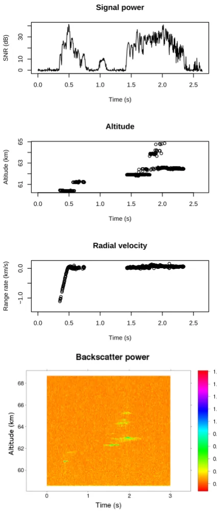
The results in of the moving point and spread target esti-mates are shown in Fig. 5. The moving point-model indicates that after the initial deceleration, the trails have nearly zero

(7)

J. Vierinen: Fractional baud-length coding 1195 Doppler shift. The spread target results show that there are up

to seven different layers separated in altitude. The strongest layer also shows range spread up to 500 m. Had a uniform baud length code with 5 µs bauds been used, the a posteriori variance would have been approximately twice larger.

This is the first time that such echos have been seen in EIS-CAT UHF observations. As micrometeoroids do not reach such a low altitude, one possible explanation is that this is a larger object. Perhaps a bolide. Because the altitude of this mono-static detection was obtained assuming that the target was within the main lobe of the antenna, another possible ex-plantion is that this is a far side lobe detection of a combined meteor head and specular trail echo directly above the radar at approximately 85–90 km altitude. However, this would re-quire the target to be approximately 45◦_{off axis.}

Meteor trail echos are not typically observed in EISCAT UHF observations as the high latitude location does not al-low observing magnetic field-aligned irregularities. Also, the trail electron density is typically too small to be observed at UHF frequencies, making observation of specular trail echos unlikely.

Recent observations at Jicamarca (Malhotra and Mathews, 2009) have indicated a new type of scattering mechanism that does not yet have a physical explanation. These so called Low Altitude Trail Echos (LATE) seem to have no preference to the angle between the magnetic field and radar beam. They also have different characteristics than specular trail echos as they are typically observed only at low altitudes, usually to-gether with head echos. Malhotra and Mathews (2009) sug-gest that these echos are produced as a by-product of frag-mentation. Our results show that there are at least seven dis-tinct layers, which is an indication that the meteor has frag-mented multiple times. However, this event is different from those described by Malhotra and Mathews in the sense that this trail is at a much lower altitude (60–65 km) and also the trail is more long lasting. So it is difficult to say if the same scattering mechanism applies here.

8 Conclusions

In this paper, we first describe the statistical theory of es-timating coherent and incoherent radar targets in amplitude domain. We then study target amplitude domain estimation variance for different codes. Using these results, we show that when sub baud-length resolution is needed, a transmis-sion code that has non-uniform baud length results smaller estimation variance than a traditional code with uniform baud lengths. We then discuss a numerical method for finding suitable constrained transmission codes. The principles are demonstrated using simulated and real coherent radar echos. The main application of non-uniform baud-length coding will be in cases where there is good SNR and sufficient receiver bandwidth, but a limited transmission bandwidth. Although the examples in this study only deal with

coher-8 J. Vierinen et al.: Fractional baud-length coding

0.0 0.5 1.0 1.5 2.0 2.5

0

10

30

Signal power

Time (s)

SNR (dB)

● ●●●●●●●●●●●●●●●●●●●●●●●●●●●●●●●●●●●●●●●●●●●●●●●●●●●●●●●●●●●

●●●

● ●●● ● ● ●●●●●●●●●●●●●●●●●●●●●●●●●●

● ● ● ●●●●●●●●●●●●●●●●●●●●●●●●●●●●●●●●●●●●●●●●●●●●●●●●●●●●●●

● ● ● ●●●●●●●●●●●●●

● ●● ● ● ● ● ●●●●●●●●●

● ●●●● ● ● ● ●● ● ●●●●●●●●●

●

● ● ● ●●

● ●

● ● ● ●●●●●

● ● ● ●

● ● ● ● ●●● ● ● ● ●

● ● ● ● ● ●

●●●●● ● ● ●●●● ● ● ●

● ●

● ●●● ●

● ● ●

● ● ● ●●●●●●●●●

●

●●●●●●●●●●●●●●●●●●●●●●●●●●●●●●●●●●●●●●●●●●●●●●●●●●●●●●●●●●●●●●●●●●●●●●●●●●●●●●●●●●●●●

0.0 0.5 1.0 1.5 2.0 2.5

61

63

65

Altitude

Time (s)

Altitude (km)

● ●●●●● ● ●●●●●●●

●●●●●●●●●●●●●●●●●●●●●●●●●●●●●●●●●●●●●●●●●●●●●●●●●●●●●_● ●

●●●●●●●●●●●●●●●●●_●●●●_●●●●● ●●●●●●●●●●●●●●●●●●●●●●●●●●●●●●●●●●●●●●●●●●●●●●●●●●●●●●●●●●●●●●●●● ● ●

●●●●●●●●●●●_●●●●●●●●●●●●●●●●●●●●●●●●●●●●●●●●●●●●●●●●_●●●●●●●●●●●●_●●●●●●●●●●●●●●●●●●●●●●●●●●●●●●●●●●●●●●●●●●●●●●●●●●●●●●●●●●●●●●●●●●●●●●●●●●●_●●●●●●●●●●●●●●●●●●●●●●●●●●●●●●●●●●●●●●●●●●●●●●●●●●●●●●●●●●●●●●●

0.0 0.5 1.0 1.5 2.0 2.5

−1.0

0.0

Radial velocity

Time (s)

[image:7.595.318.531.72.580.2]

Range rate (km/s)

Fig. 5.A low-altitude meteor echo at 60 km seen with the EISCAT UHF radar on 19.11.2009 at 5:16 UT during a low-elevation meteor experiment. The meteor echo can been decelerating from 1 km/s down to 0, and then then echos from a trail-like structure are seen for a while. The three top panels show the results from a moving point-target model that determines the most likely range, Doppler shift and power of a point target. The fourth panel shows the range resolved backscatter power from a spread target model. After the initial head echo, many layers appear at altitudes above the initial detection. Most of the layers show 100-400 m range spread. Fig. 5. A low-altitude meteor echo at 60 km seen with the

EIS-CAT UHF radar on 19 November 2009 at 05:16 UT during a low-elevation meteor experiment. The meteor echo can been

decelerat-ing from 1 km s−1down to 0, and then then echos from a trail-like

(8)

1196 J. Vierinen: Fractional baud-length coding ent targets, the considerations also apply for amplitude

do-main estimation of strong range and Doppler spread (inco-herent) echos, such as the ones described in Vierinen et al. (2008b). Examples of practical use cases include Lunar mea-surements, range spread meteor trail studies, and artificial ionospheric heating induced enhanced ion- and plasma-line echos.

Non-uniform baud-lengths are also advantageous for multi-purpose high power large aperture radar experiments where one mainly observes targets that benefit from longer baud lengths (e.g., ionospheric plasma or space debris), but where one would still want to be able to analyze strong tar-gets at sub-baud resolution.

Although we have only studied the non-uniform baud-length coded transmission envelope performance in the case of amplitude domain target estimation, the same principles can also be applied to find optimal high resolution transmis-sion codes for lag-profile invertransmis-sion (Virtanen et al., 2008c) using estimation variance calculations that can be found e.g., in Lehtinen et al. (2008).

Acknowledgements. Editor-in-Chief M. Pinnock thanks J. Sahr and another anonymous referee for their help in evaluating this paper.

References

Cooley, J. W. and Tukey, J. W.: An algorithm for the machine cal-culation of complex fourier series, Math. Comput., 19, 297–301, 1965.

de Boor, C.: A Practical Guide to Splines, 114–115 pp., Springer-Verlag, 1978.

Farley, D. T.: Multiple-pulse incoherent-scatter correlation function measurements, Radio Sci., 7(6), 661–666, 1972.

Kelleher, J. and O’Sullivan, B.: Generating all partitions: A com-parison of two encodings, CoRR, abs/0909.2331, 2009. Kirkpatrick, S., Gelatt, C. D., and Vecchi, M. P.:

Optimiza-tion by Simulated Annealing, Science, 220(4598), 671–680, doi:10.1126/science.220.4598.671, 1983.

Kudeki, E. and Stitt, G. R.: Frequency domain interferometry: A high resolution radar technique for studies of atmospheric turbu-lence, Geophys. Res. Lett., 14(3), 198–201, 1987.

Lehtinen, M. S., Damtie, B., and Nygr´en, T.: Optimal binary phase codes and sidelobe-free decoding filters with applica-tion to incoherent scatter radar, Ann. Geophys., 22, 1623–1632, doi:10.5194/angeo-22-1623-2004, 2004.

Lehtinen, M. S., Virtanen, I. I., and Vierinen, J.: Fast comparison of IS radar code sequences for lag profile inversion, Ann. Geophys., 26, 2291–2301, doi:10.5194/angeo-26-2291-2008, 2008.

Malhotra, A., and Mathews, J. D.: Low-altitude meteor trail echoes, Geophys. Res. Lett., 36, L21106, doi:10.1029/2009GL040558, 2009.

Nikoukar, R.: Near-optimal inversion of incoherent scatter radar measurements: coding schemes, processing techniques, and experiments, PhD thesis, University of Illinois at Urbana-Champaign, 2010.

Piiroinen, P.: Statistical measurements, experiments and applica-tions, Academia Scientiarum Fennica, 2005.

Pirttil¨a, J. and Lehtinen, M.: Solving the range-doppler dilemma with ambiguity-free measurements developed for incoherent scatter radars, COST 75, Advanced Weather radar systems, In-ternational seminar, pp. 557–568, 1999.

Pukelsheim, F.: Optimal Design of Experiments, John Wiley & Sons, 1993.

Riha, W. and James, K. R.: Algorithm 29 efficient algorithms for doubly and multiply restricted partitions, Computing, 16, 163– 168, doi:10.1007/BF02241987, 1976.

Ruprecht, J.: Maximum-Likelihood Estimation of Multipath Chan-nels, PhD thesis, Swiss federal institute of technology, 1989. Sahr, J. D. and Grannan, E. R.: Simulated annealing searches for

long binary phase codes with application to radar remote sensing, Radio Sci., 28(6), 1053–1055, doi:10.1029/93RS01606, 1993. Shapiro, H. S. and Silverman, R. A.: Alias-free sampling of random

noise, Journal of the Society for Industrial and Applied Mathe-matics, 8(2), 225–248, 1960.

Sulzer, M. P.: Recent incoherent scatter techniques, Adv. Space Res., 9, 153–162, 1989.

Uppala, S. V. and Sahr, J. D.: Spectrum estimation of moderately overspread radar targets using aperiodic transmitter coding, Ra-dio Sci., 29, 611–623, 1994.

Vierinen, J., Lehtinen, M. S., Orisp¨a¨a, M., and Damtie, B.: Gen-eral radar transmission codes that minimize measurement error of a static target, arxiv:physics/0612040v1, published on-line at arxiv.org, 2006.

Vierinen, J., Lehtinen, M. S., Orisp¨a¨a, M., and Virtanen, I. I.: Transmission code optimization method for incoherent scatter radar, Ann. Geophys., 26, 2923–2927, doi:10.5194/angeo-26-2923-2008, 2008a.

Vierinen, J., Lehtinen, M. S., and Virtanen, I. I.: Amplitude do-main analysis of strong range and Doppler spread radar echos, Ann. Geophys., 26, 2419–2426, doi:10.5194/angeo-26-2419-2008, 2008b.

Virtanen, I. I., Lehtinen, M. S., Nygrén, T., Orispää, M., and Vieri-nen, J.: Lag profile inversion method for EISCAT data analysis, Ann. Geophys., 26, 571–581, doi:10.5194/angeo-26-571-2008, 2008c.