Speech signal modeling using multivariate distributions

R E S E A R C H

Open Access

Speech signal modeling using multivariate

distributions

Ali Aroudi

, Hadi Veisi

, Hossein Sameti

and Zahra Mafakheri

Abstract

Using a proper distribution function for speech signal or for its representations is of crucial importance in statistical-based speech processing algorithms. Although the most commonly used probability density function (pdf) for speech signals is Gaussian, recent studies have shown the superiority of super-Gaussian pdfs. A large research effort has focused on the investigation of a univariate case of speech signal distribution; however, in this paper, we study the multivariate distributions of speech signal and its representations using the conventional distribution functions, e.g., multivariate Gaussian and multivariate Laplace, and the copula-based multivariate distributions as candidates. The copula-based technique is a powerful method in modeling non-Gaussian multivariate distributions with non-linear inter-dimensional dependency. The level of similarity between the candidate pdfs and the real speech pdf in different domains is evaluated using the energy goodness-of-fit test.

In our evaluations, the best-fitted distributions for speech signal vectors with different lengths in various domains are determined. A similar experiment is performed for different classes of English phonemes (fricatives, nasals, stops, vowels, and semivowel/glides). The evaluation results demonstrate that the multivariate distribution of speech signals in different domains is mostly super-Gaussian, except for Mel-frequency cepstral coefficient. Also, the results confirm that the distribution of the different phoneme classes is better statistically modeled by a mixture of Gaussian and Laplace pdfs. The copula-based distributions provide better statistical modeling of vectors representing discrete Fourier transform (DFT) amplitude of speech vectors with a length shorter than 500 ms.

Keywords:Multivariate distribution of speech signal, Copula-based multivariate distribution, Mel-frequency cepstral coefficient (MFCC), Discrete cosine transform (DCT), Discrete Fourier transform (DFT), Linear predictive coefficient (LPC), Goodness-of-fit (GOF) test

1 Introduction

Statistical-based speech processing algorithms have attracted wide interests during the last three decades in numerous applications, e.g., speech coding [1], speech recognition [2, 3], speech synthesis [4], and speech enhancement [5]. In all statistical-based speech process-ing algorithms, a probability density function (pdf ) is assumed for the signal or its representation. Therefore, it is not surprising that proper selection of the pdf has been one of the challenges persistently addressed in this area [6–8].

Most of the statistical-based speech processing algo-rithms assume Gaussian probability distribution density

for speech signals [2, 9–13]. The simplicity of the formu-lations and the semi-support of the central limit theorem are the main motivations for using Gaussian pdf [14]. Recently, a number of researchers have studied the distribution of speech signal more precisely using goodness-of-fit (GOF) test [15, 16] in time domain and transformed domains, e.g., discrete cosine transform (DCT) and discrete Fourier transform (DFT). In this regard, Gazor et al. [14], Martin [6], Shin et al. [7], Chen and Loizou [17], and Erkelens et al. [18] have shown that speech signals in various domains are modeled more accurately by super-Gaussian pdfs than by Gaussian pdf. Their evaluation results have demonstrated that the pdf of speech signals for time and DCT features are closer to Laplace [14], for jointly amplitude and phase of DFT features are closer to complex Laplace [17], for ampli-tude of DFT features are closer to Rayleigh [18], and for * Correspondence:[email protected]

2_{Faculty of New Sciences and Technologies, University of Tehran, Tehran,}

Iran

Full list of author information is available at the end of the article

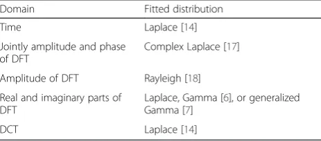
real or imaginary parts of DFT features are individually closer to either Laplace or Gamma [6]. In addition, Shin et al. [7] have reported that generalized Gamma pdf models the distribution of real parts of DFT features more accurately compared to the Gaussian pdf. Table 1 summarizes the results of the published evaluations in this field.

All aforementioned publications have aimed to address the issue of modeling univariate pdf of speech signals for algorithms using univariate pdf. However, there are many statistical-based algorithms that take advantage of multivariate distribution of speech signals, and therefore, studying the multivariate distribution of speech to ex-ploit a more proper pdf is a key issue for those speech processing algorithms too. There are typically several challenges in the studying and modeling of speech signals in the multivariate distribution case, e.g., the non-linear or linear inter-dimensional dependency, and the sparsity and complexity of the multidimensional space. These issues may have caused to mostly focus on the investigation of univariate distribution during the last two decades, and a small progress has been made in the multivariate distribution study of speech signal. The earlier studies on multivariate distribution of speech signal, performed by Brehm et al. [19] and LeBlancin et al. [20], suggested the multivariate Gaussian pdf for speech frames with a length of 5 ms. As the frame length and the process domain may vary the distribution [14], the multivariate Gaussian pdf may not be an appropriate choice for the algorithms using frame length other than 5 ms, e.g., 10 to 35 ms or exploiting process domain other than the time domain, e.g., DFT or DCT. In re-cent studies, Gazor et al. [14] and Jensen et al. [21] have used the moment test and have shown that Laplace multivariate distribution models speech signal or its representations are better than the Gaussian multi-variate distribution. However, in these studies, the moment test as a GOF test was applied to each dimension individually and the possible contribution of inter-dimensional dependency to the multivariate distribution was not considered.

In this paper, we investigate multivariate distribution of speech signal in the time and transformed domains. We consider new plausible distribution candidates to tackle the multivariate distribution modeling challenges. Among the candidates, copula-based distributions are also proposed which are able to model the high-dimensional non-Gaussian distribution with non-linear inter-dimensional dependency [22]. The copula-based distributions have been popular over the last decade in the statistical fields, e.g., climate research, econometrics, risk management [22, 23], and finance [24, 25]. The other possible pdf candidates of speech including multi-variate Gaussian, multimulti-variate Laplace, the mixture of Gaussian, and the mixture of Laplace distributions are investigated in this paper too. We employ the goodness-of-fit test [15, 16, 26] to evaluate the degree of similarity between the candidate distribution and the real speech signal distribution. The GOF test is a tractable three-step approach to investigate distribution of data. In the first step, a number of candidates are assumed as the pdf of the real data. Next, an estimator, e.g., maximum likeli-hood (ML) is exploited to fit the candidates to the real data, and finally, the GOF test is performed to quantify the level of similarity between the fitted candidates and the real data. It is noted that although a wide number of GOF tests have been proposed, the most appropriate GOF test is the one that can highly cover underlying problem conditions, e.g., in our case study is high dimensionality of spaces. We briefly present a number of GOF tests, a summary of their strengths and deficien-cies, and finally choose the one that has been reported as the most appropriate for high-dimensional space.

In general, speech processing algorithms using multi-variate distribution exploit different feature types to process speech signals. For instance, traditional hidden Markov model (HMM)-based speech recognition and synthesis algorithms [3, 27] exploit Mel-frequency cepstral coefficients (MFCC); HMM-based speaker recognition [13] systems exploit either linear predictive coding (LPC) or MFCC; HMM-based speech enhancement algorithms use LPC, time, DCT, MFCC, or DFT [7, 9, 10]; and codebook-driven-based speech enhancement algorithms [28] employ LPC. However, all these algorithms assume the multivariate Gaussian pdf for extracted features of speech signals. As the feature type may influence the distribution [14], the multivariate distribution of the different feature types including DFT, DCT, time, LPC, and MFCC is studied in this paper. It is noted that a number of speech processing algorithms, e.g., proposed by Martin [6], Shin et al. [7], model the real and imaginary parts of DFT separately. Thus, we study the real and imaginary parts of DFT features separately. The whole study of multivariate distribution in this paper is concen-trated on clean speech signals.

Table 1Proposed super-Gaussian univariate distribution of speech signal in different domains

Domain Fitted distribution

Time Laplace [14]

Jointly amplitude and phase of DFT

Complex Laplace [17]

Amplitude of DFT Rayleigh [18]

Real and imaginary parts of DFT

Laplace, Gamma [6], or generalized Gamma [7]

The remainder of this paper is structured as follows. In Section 2, the copula-based distributions are pre-sented including their formulations and parameter esti-mation. In Section 3, the GOF tests are briefly reviewed and among them, the energy test is selected as the most appropriate one for the multivariate distribution study of high-dimensional space. Section 4 elaborates candidates’ formulations, their parameter estimation, and an algo-rithm for exploring the best-fitted candidate. Section 5 presents the evaluation setup and experimental results. Finally, Section 6 concludes the work.

2 Copula-based distribution

A copula is defined as a multivariate probability distribu-tion where the marginal probability distribudistribu-tion of each variable is uniform and is used to describe the depend-ency between random variables [22, 29–33]. As all the multivariate joint distributions can be written in terms of a copula and univariate marginal pdfs [29], copulas are used as a popular statistical tool for modeling multi-variate distributions. In this regard, copulas allow to easily model the distribution of multivariate random variables by estimating only marginal pdfs and copulas. A copula-based distribution can capture important char-acteristics of a vector, e.g., the appropriate pdf for mar-gins and the appropriate correlation structure with a possibly simple form.

The purpose of this section is to briefly review the basic definition of the copula and a number of the most commonly used estimation methods for fitting the copula to the real data.

2.1 Copula model

The mathematical basis of the copula was proposed by Sklar [29] and Hoeffding [33]. To define a copula model, let x be a d-dimensional random vector x= {x1,…,xj,…,xd}. Sklar [29] showed that the joint cumulative distribution function (CDF) ofx,FX(x), can be expressed as a function of marginal CDFs uj¼FXj xj ; j¼1:d, as shown in Eq.

(1), where CX: [0, 1]d→[0, 1] denotes copula function. Based on Sklar’s theorem [29], any arbitrary multivariate pdffX(x) can be expressed as the product of two terms: the marginal pdf of dimensions fXj xj ; j¼1:d and the

copula density functioncX(.) as shown in Eq. (2). The cop-ula density functioncX(.) can be derived from the copula function as given in Eq. (3). As the copula density function characterizes the inter-dimensional dependencies, it is also called correlation structure in literature [22].

FXð Þ ¼x CX u1;…;uj;…;ud

ð1Þ

fXð Þ ¼x Yd

j¼1 fXj xj

!

:cX u1;…;uj;…;ud

ð2Þ

cX u1;…;uj;…;ud

_¼ Yd

j¼1

∂ ∂uj

!

:CX u1;…;uj;…;ud

ð3Þ

The two most used parametric forms forcX(.) are ellip-tical and Archimedean [22, 30]. The Archimedean-based copulas are mostly used in the bivariate form and they are not practically usable for high-dimensional spaces due to its high-computational cost [22, 34]. In contrast to the Archimedean, the elliptical-based copulas, includ-ing Gaussian and Student-t copula, can be used for spaces with any number of dimensions [22]. We there-fore briefly review the Gaussian and Student-t copulas in the following sections.

2.2 Gaussian copulas

Let us assume the marginal CDFs, uj, are known. Each

ujcan be transformed to a standard distributed random variable yj, by using the inverse of univariate Gaussian CDFF−1

Nð0;1Þð Þ: as shown in the following equation,

yj¼F−N1ð0;1Þ uj ¼F−N1ð0;1Þ

FXj xj eNð0;1Þ: ð4Þ

As a consequence, the set y= {y1,…,yj,…,yd} has a multivariate Gaussian distribution N(0,ΣCopula), where

ΣCopula denotes a symmetric, diagonal, positive definite matrix with unit diagonal elements. The joint CDF of y can therefore be expressed by Eq. (5), which can be interpreted as the copula function ofxusing terminology of Eq. (1). By using Eqs. (3) and (5), the copula density can be derived as shown in Eq. (6), whereIdenotes an identity matrix and Tr denotes transpose operator. For further details on this topic, see [22] and [31].

FXð Þ ¼x CX u1;…; :uj; ::;ud

¼FNð0;ΣCopulaÞðy1;…;yj;…;ydÞ ð5Þ

cXðu1;…;udÞ ¼ 1

ΣCopula

0:5 exp −

1 2 y Σ

−1 Copula−I

yTr

ð6Þ

2.3 Student-t copulas

The Student-t copula is defined analogously to the Gaussian copula; however, the transformed variables yj are obtained using univariate Student-t CDF inverse F−1

t vð Þ uj , wheret(v) is a univariate Student-t distribution

the Student-t copula density then is computed as shown in Eq. (8). For further details, see [22] and [31].

CXðu1;…;udÞ ¼Ftðv;ΣCopulaÞ F

−1

t vð Þð Þu1 ;…;F−_{t v}ð Þ1 ð Þud

ð7Þ

cXðu1;…;udÞ ¼ΣCopula−0:5

Γ vþd 2

Γ v 2

d

Γ vþ1 2 d Γ v 2 1þ 1 vyΣ−

1 Copulayt

−vþd

2

Yd

j¼1 1þy

2

v

−vþ1

2

ð8Þ

2.4 Fit a copula model

There are several estimation methods proposed for copula parameters [22, 35–37]. Among them, maximum likelihood (ML), inference functions for margins (IFM), and canonical maximum likelihood (CML) techniques are used more frequently than others [22]. Generally, these estimators maximize the log-likelihood function of Eq. (2) with respect toΘ¼fθ;αgin different ways, where α denotes a set of parameters concerning the copula density function, e.g.,ΣCopula, andθ= {θ1,…,θj,…,θd} de-notes a set of parameters concerning the marginal pdfs, fXj xj . The log-likelihood function is derived as shown in

Eq. (9) [31] where xN

n¼1¼fx1;…;xn;…;xNg denotes a

set ofNobservation vectors of real data andxn

j represents jth component of vectorxn.

lð Þ ¼Θ

∑

n¼1

N Xd

j¼1 lnfXj x

n j;θj

þXN

n¼1

lnc FX1 x

n

1;θ1

;…;FXj x n j;θj

;…;FXd x n d;θd

;α

h i

ð9Þ

The ML approach estimates the parameters of mar-ginal pdfs and copula density function jointly using numerical optimization [22]. This is the only way to estimate all the parameters consistently [22].

The IFM method is the most used method. It esti-mates by maximizing Eq. (9) in two steps. First, the parameters of the marginsθare individually estimated as shown in Eq. (10). It is noted that the type of marginal distributions, e.g., Laplace or Gamma, are assumed to be determined in advance. The copula parameters αare then derived as shown in Eq. (11) by using the estimatedθ^.

^

θj¼ arg max XN

n¼1

lnf_Xj xn j;θj

ð10Þ

^

α¼arg max X N

n¼1

lnc FX1 x n

1; ^θ1

;…;FXj x

n j; ^θj

;…;FXd x

n d; ^θd

;α

" #

ð11Þ

The CML method first empirically estimates fXj x n j

and _FXj xnj , denoted as f^Xj x n

j and F^Xj xnj , using

non-parametric methods, e.g., kernel smoothing density estimator [38]. Thus, it is not needed to determine the type of marginal distributions in advance, in contrast to the IFM method. The parameters of copula are then estimated using Eq. (12).

^

α¼arg max X

N

n¼1

lnc F^X1 x

n

1 ;…;F^Xj x n

j ;…;F^Xd x n d ;α

" #

ð12Þ

In order to estimate the parameters of the copula-based distribution using one of the discussed methods, the following issues should be considered:

– The ML method is used for spaces with a small number of dimensions due to the numerical complexity issue.

– The IFM method ends up a sub-optimal solution for parameter estimation since the log-likelihood function is maximized in two individual steps [31].

– The IFM and CML methods result in closed-form formulas only for Gaussian copula case [31].

– When one of the values of off-diagonal compo-nents of the covariance matrix ΣCopula of either the Student-t or Gaussian copulas takes 1 or −1, the estimation procedure of the copula parame-ters using CML method may fail [39]. It is due to Cholesky decomposition performed in CML methods.

In this paper, the parameters of copula-based dis-tributions are estimated using IFM method and Gaussian copula density function that result in closed-form formulas and avoid failing in the esti-mation procedure. To estimate α=ΣCopula of Gauss-ian given a vector sequence yN

n¼1¼fy1;…;yn;…;yNg

^ ΣCopula¼

1 N

XN

n¼1 yn

ð ÞT r_yn _ð13Þ

3 Goodness-of-fit test

A wide number of goodness-of-fit (GOF) tests depend-ing on underlydepend-ing conditions of the case study have been proposed. In our study, high dimensionality and possible non-linear inter-dimensional dependency are the most crucial issues. Although various GOF tests are proposed for one-dimensional space, only some of them are extendable for high-dimensional space. As the number of space dimensions increases, the tests become ineffi-cient [26]. For instance, the extension of χ2 test [15] to higher dimensions suffers from the curse of dimension-ality [40] caused by the space sparsity unless the sample sizes are large enough.

There are several GOF tests particularly proposed for the multivariate case, e.g., the nearest neighbor test which exploits the nearest neighbors [41], Mardia test which exploits the skewness and kurtosis [42] and Freidman– Rafsky test which exploits the minimum spanning tree [43]. In this regard, the energy test has also recently been proposed by Zach and Aslan [44]. The performance superiority of the energy test has been demonstrated compared to Mardia, nearest neighbor,χ2, and Friedman– Rafsky tests. Accordingly, the energy test is selected as a more appropriate GOF for underlying conditions of the study in this paper to evaluate candidates. In the follow-ing, the energy test is discussed.

3.1 Energy test

Given a candidate pdf _fX0ð Þx and a sequence of obser-vation vectors xN

n¼1¼fx1;…;xi;…;xNg which follow

an unknown pdf fX(x), the energy statistic for the hypothesis H0:fXð Þ ¼x f_X0ð Þx against H1:fXð Þx ≠f_X0ð Þx is

computed by

ϕNM¼

1 N Nð −1Þ

X

t>i

Rxi−xt

þ 1

M Mð −1Þ

X

j>n

R q n_−qj

− 1

NM

XN

i¼1

XM

j¼1

Rxi−qj

ð14Þ

where qM_j¼1¼fq1;…;qj;…;qMg denotes a sequence of Mobservation vectors followingfX0ð Þx and generated by

Monte–Carlo simulation [45] and R denotes a continu-ous, monotonically decreasing function, i.e.,R(r) =−ln(r). In the limit N→∞ and M→∞, the statistic ϕNM ap-proaches minimized value, near zero, ifxN_i¼1 and qMj¼1 are

from the same distribution [44]. For further details, see theAppendix.

The required steps for performing the energy test are summarized:

1. The real dataset is segmented, resulting inNvectors each of lengthd,xNi¼1¼fx1;…;xi;…;xNg.

Depending on the process domain,_xirepresents the segmented real data in that process domain, e.g., time, DFT, and DCT.

2. A possible candidate pdf_fX0ð Þ_x , e.g., either copula-based or conventional distributions, is hypothesized and fitted to the real data vectorsxNi¼1.

3. The number_Mof simulated data vectors following fitted pdffX0ð Þx is generated using Monte–Carlo.

4. The energy test statistic is computed using Eq. (14) to determine the level of similarity between the distributions of real data vectorsxNi¼1and simulated

data vectorsqMj¼1.

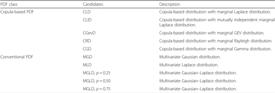
4 Multivariate distribution candidates

To study the multivariate distribution of speech features, two classes of pdfs are considered as the candidates in this paper: (1) copula-based distributions and (2) con-ventional distributions. The first pdf class includes five distributions:

1. Copula-based Laplace distribution (CLD) 2. Copula-based Laplace distribution with mutually

independent dimensions (CLID), i.e.,cX(.) = 1

3. Copula-based generalized extreme value distribution (CGevD)

4. Copula-based Rayleigh distribution (CRD) 5. Copula-based Gamma distribution (CGD).

As formerly mentioned, the IFM method is used to fit the copula-based distributions to real data. In this re-gard, marginal distributions of each candidate should be first determined. The following univariate pdfs are used as the marginal distributions for each candidate: univari-ate Laplace pdf as shown in Eq. (15) [14] for CLD and CLID, univariate generalized extreme value pdf as shown in Eq. (16) [46] for CGevD, univariate Rayleigh pdf as shown in Eq. (17) for CRD, and univariate Gamma pdf as shown in Eq. (18) [21] for CGD. In these equations, μj and αj denote the location parameters, bj, ξj, and σj denote the scale parameters, and kj and γjrepresent the shape parameters. As a consequence, CLD is a copula-based distribution with marginal distributions of Laplace and its parametersΘCLD= {θLaplace,αCopula} are estimated using the IFM method given an observation set of vectors xN

fXj;Laplace xj ; j¼1:d and is estimated using Eqs. (19)

and (20). The parameter of Gaussian copula density αCopula is estimated using Eq. (13). Similarly, θRayleigh = {νj} is estimated using Eq. (21) and θGamma= {γj,ξj} is estimated using Eqs. (22) and (23) [47], where

s¼ ln 1

N XN

n¼1

xn j ! −1 N: XN

n¼1 ln xn

j . It is noted that CGD and

CRD both model one-side distributions and are therefore proposed as candidates for modeling one-side distributed random vector, e.g., the amplitude of DFT feature. For estimation of CGevD parameters θGEV= {σj,αj,kj} using the IFM, as it results in no closed-form solution [48], the MATLAB function “fminsearch”, which employs numerical method of Lagarias [49], is employed.

fXj;Laplace xj ¼

1

2bj:exp −

xj−μj bj 0 @ 1

A ð15Þ

fXj;GEVxj ¼

1 σj :exp −

1þkjxj_σ−αj j

−1

kj!

: 1þkj

xj−μj

σj 0 @ 1 A −1−1 kj

ð16Þ

fXj;Rayleigh xj ¼

x

ν2

j

:exp −x 2

2ν2

j !

ð17Þ

fXj;Gamma xj ¼

xj γj−

1

ξj

γ_j

Γ γj

:exp −_ξxj

j

ð18Þ

^

μ_j¼median xnj ð19Þ

^

bj¼

1 N:

XN

n¼1 xnj−μj

ð20Þ

^ νj≈

ffiffiffiffiffiffiffiffiffiffiffiffiffiffiffiffiffiffiffiffiffiffiffiffiffiffiffiffiffi

1 2N:

XN

n¼1 xn_j 2

v u u

t _ð21Þ

^ γj≈

3−sþ

ffiffiffiffiffiffiffiffiffiffiffiffiffiffiffiffiffiffiffiffiffiffiffiffiffiffiffi

s−3

ð Þ2_þ

24s

q

12s

ffiffiffiffiffiffiffiffiffiffiffiffiffiffiffiffiffiffiffiffiffiffiffiffiffiffiffiffiffi

1 2N:

XN

n¼1 xnj

2

v u u

t _ð22Þ

^

ξj¼

1

γjN :XN

n¼1

xnj ð23Þ

The following steps summarize the estimation proced-ure of Gaussian copula.

1. A marginal distribution, e.g., one of Eqs. (15)–(18), is accounted forfXj xj ; j¼1:dand parameter set is

accordingly estimated.

2. The corresponding CDF offXj xj is derived to

computeuj¼FXj xj ; j¼1:dandyj¼F−N1ð0;1Þ uj

as shown in Eq. (4).

3. The parameter of Gaussian copula density

αCopula=ΣCopula is estimated using Eq. (13).

The second class of candidate distributions, i.e., con-ventional distributions, includes five concon-ventional pdfs: multivariate Laplace (MLD), multivariate Gaussian (MGD), and three multivariate Gaussian–Laplace mix-tures (MGLD). The MGD is considered as shown in Eq. (24) where the full covariance matrixΣand mean vector μ are estimated using the maximum likelihood method [16]. Regarding MLD, as the ultimate purpose is to compute the energy test statistic using simulated vectors following MLD, the required vectors si

Laplace are generated using Eq. (25) [50] wherexi_Gaussian andwidenote simulated vector following MGD of Eq. (24) and simulated sample following univariate exponential distribution of Eq. (26),

Table 2Multivariate distribution candidates considered for experimental setup

PDF class Candidates Description

Copula-based PDF CLD Copula-based distribution with marginal Laplace distribution.

CLID Copula-based distribution with mutually independent marginal

Laplace distribution.

CGevD Copula-based distribution with marginal GEV distribution.

CRD Copula-based distribution with marginal Rayleigh distribution.

CGD Copula-based distribution with marginal Gamma distribution.

Conventional PDF MGD Multivariate Gaussian distribution.

MLD Multivariate Laplace distribution.

MGLD,p= 0.25 Multivariate Gaussian–Laplace distribution.

MGLD,p= 0.50 Multivariate Gaussian–Laplace distribution.

respectively. For MGLD observations, the simulated vectors are generated using Eq. (27) where siLaplace and xi

Gaussian denote the simulated vectors following distribu-tions of Eqs. (25) and (24), respectively. In this equation, variable pshows the amount of contribution of Laplace distribution compared with Gaussian distribution in generating zi. Three multivariate Gaussian–Laplace mixtures are considered with corresponding values of p∈{0.25, 0.50, 0.75}, denoted as MGLD with p= 0.25, MGLD with p= 0.50, and MGLD with p= 0.75, for the experimental evaluations.

f_X;Gaussianð Þ ¼x 1

ffiffiffiffiffiffiffiffiffiffiffiffiffiffiffiffiffi Σ

j jð Þ2π d

q :exp −1

2ðx−μÞΣ

−1_ðx−μÞt

ð24Þ

si Laplace ¼

ffiffiffiffiffi

wi

p xi

Gaussian ð25Þ

fExponentialð Þ ¼wi

1

λ exp

−wi

λ

ð26Þ

zi_¼psi

Laplaceþð1−pÞxi_Gaussian ð27Þ

Consequently, eight candidates are considered for multivariate distribution study of speech features, ex-cept for amplitude of DFT feature. For the amplitude of DFT feature, two additional candidates CGD and CRD resulting in total ten candidates are considered. Table 2 summarizes the candidates.

5 Evaluation results

In this section, the experimental evaluation results of the multivariate speech distribution study are presented. To perform the evaluations, 100 sentences, uttered by 11 male and female native English speakers (with New York City dialect region), with sampling rate of 16 kHz from TIMIT database [51] were randomly selected (see Additional file 1). Two experimental setups were considered for eval-uations. For the first experimental setup, all speech infor-mation of 100 sentences was exploited for computing the statistic of the energy test. For the second experimental setup, phoneme-based evaluations were performed, i.e., five classes of English phonemes were used (fricatives, na-sals, stops, vowels, and semivowel/glides). For each phon-eme class, the relevant information was first extracted from the 100 sentences used in the first experimental setup and then concatenated to produce one file. As a re-sult, five output files for five phoneme classes were pro-duced. Table 3 shows the content and the number of extracted phonemes of each of the five files. The evalu-ation results of the second experimental setup benefit the statistical-based speech recognition and synthesis algo-rithms statistically modeling phoneme classes. As non-speech information (silence interval) may influence the distribution [14], it was removed for both experimental setups. The total duration of the first setup data after excluding silence intervals was 337.84 s. For the second setup, the duration of each file is represented in Table 3.

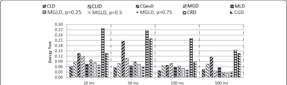
Fig. 1Values of the energy test for different multivariate distributions (candidates) resulted from ADFT features with frame lengths of 20, 30, 100, and 500 ms

Table 3The data set of the second setup of evaluations

File Phoneme class # of phonemes Duration (s) # of frames for each phoneme class (N)

20 ms 30 ms 100 ms 500 ms

1 Semivowel/glide 460 29.77 1489 993 298 60

2 Vowel 1240 125.39 6270 4180 1254 251

3 Nasal 298 18.57 929 620 186 38

4 Fricative 482 46.16 2309 1539 462 93

a

b

c

d

e

f

Prior to performing evaluation, the datasets of both setups were segmented in frames with lengths of 20, 30, 100, and 500 ms. For the first setup, the number of frames, N, corresponding to the segment lengths of 20, 30, 100, and 500 ms were 13936, 9291, 2788, and 558, respectively. For the second setup, the number of frames, N, corresponding to the segment lengths for each phoneme class is shown in Table 3.

The experimental evaluations were performed for time features (T), amplitude of DFT (ADFT), real parts of DFT (RDFT), imaginary parts of DFT (IDFT), DCT, LPC, and MFCC features. Regarding the LPC and MFCC, 10 and 12 coefficients were extracted from frames, respectively. The MFCC vectors were extracted from 23 Mel-frequency filter banks. To set up the energy test, the value of M was taken equal to N. All the reported energy test values were computed at a signifi-cant level of 0.01 using a bootstrap method [44, 52].

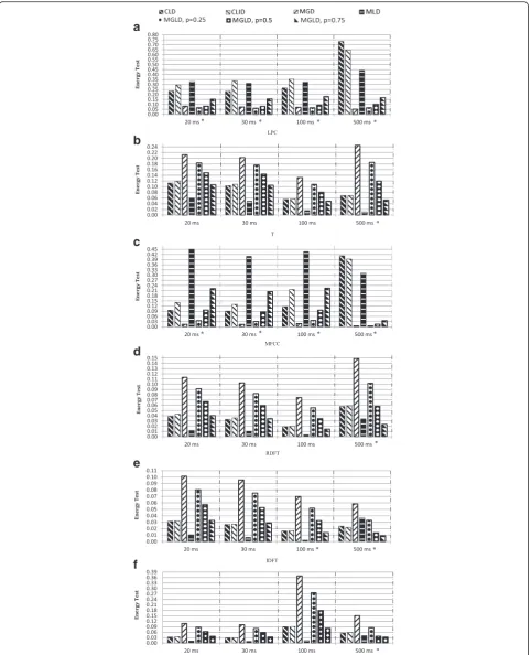
Figure 1 represents the experimental results of the energy test for ADFT features, concerning the first setup. Fig. 2 illustrates the experimental results of the energy test for other features including LPC, T, MFCC, RDFT, IDFT, and DCT features. Regarding Fig. 2, as the energy test values of some cases were much lower in comparison with the others, they were scaled up ten times to be illustrated better and punctuated by * on the right side of frame length of horizontal axis, e.g., 500 ms *. Moreover, as the energy test values of CGevD for all features were far greater than the others, they were schematically removed from Fig. 2 to have a more com-parative demonstration for the small energy test values.

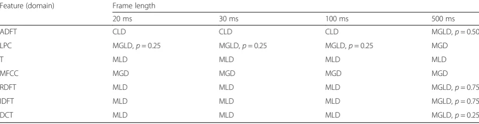
Table 4 summarizes the best-fitted candidate for differ-ent speech features and frame lengths according to Figs. 1 and 2 evaluation results. According to Figs. 1 and 2 and Table 4, the following conclusions are conducted:

– The best-fitted candidate in the sense of the energy test for the T, RDFT, IDFT, and DCT features with frame length of 20, 30, and 100 ms is MLD, despite the often used assumption of multivariate Gaussian distribution in the speech enhancement

algorithms [8–10], but consistent with the univariate Laplace distribution proposed by Martin [6] and Gazor et al. [14].

– The univariate Rayleigh distribution has been

proposed for ADFT feature with a short frame length. Maybe as a consequence, it was expected that multivariate Rayleigh distribution (CRD) would be superior in modeling the multivariate distribution of ADFT; however, the energy test evaluation results proposed the CLD as the best-fitted candidate for frame lengths shorter than 500 ms.

– Regarding statistical modeling of ADFT features with short frame length, although CLD and CLID are both Laplace-based distribution, CLD was proposed as the best-fitted candidate. As the copula density functioncX(.), which models inter-dimensional

dependency, is non-unit for CLD and unit for CLID, the superiority of CLD over CLID shows how the modeling of inter-dimensional dependency contributes to the proper multivariate statistical modeling.

– Increasing frame length to 500 ms caused the best-fitted candidate corresponding to ADFT, RDFT, IDFT, and DCT features to be shifted from either CLD or MLD toward MGLD. This finding suggests that the Gaussian distribution contributed to the actual multivariate distribution of those domains when the frame length sufficiently increased, which is also supported by the central limit theorem. Similarly, varying the best-fitted distribution for LPC features from MGLD (withp= 0.25) to MGD verifies this contribution, too.

– The best-fitted candidate for the MFCC with different frame lengths is MGD, consistent with the assump-tion of multivariate Gaussian distribuassump-tion used in most speech recognition algorithms [2,3]. Table 4Best-fitted multivariate distribution in the sense of energy test for different features and frame lengths of speech signals

Feature (domain) Frame length

20 ms 30 ms 100 ms 500 ms

ADFT CLD CLD CLD MGLD,p= 0.50

LPC MGLD,p= 0.25 MGLD,p= 0.25 MGLD,p= 0.25 MGD

T MLD MLD MLD MLD

MFCC MGD MGD MGD MGD

RDFT MLD MLD MLD MGLD,p= 0.75

IDFT MLD MLD MLD MGLD,p= 0.75

DCT MLD MLD MLD MGLD,p= 0.25

A: First best-candidate B: Second best-candidate

C= Energy test value of A D= Energy test value of B

According to the conclusions, representative frames of speech signals containing T, RDFT, IDFT, or DCT features that are often used in statistical model-based speech enhancement algorithms [9, 10, 28] can be better statistically modeled by the MLD than MGD distribu-tion. Furthermore, if the statistical-based algorithm exploits MFCC and ADFT, the energy test proposes MGD and ADFT, respectively.

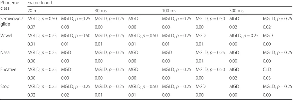
Tables 5, 6, 7, 8, 9, 10, and 11 present the evaluation re-sults of the energy test for the second experimental setup. In each table, there are 15 blocks surrounded by bold lines belonging to each phoneme class with a determined frame length. Each block in these tables contains four cells, as shown by Fig. 3. The A and B cells show the first and the second best-fitted candidates, respectively, and C and D cells indicate the energy test value cor-responding to the first and the second best-fitted can-didates, respectively.

According to Tables 5, 6, 7, 8, 9, 10, and 11, the fol-lowing conclusions are conducted:

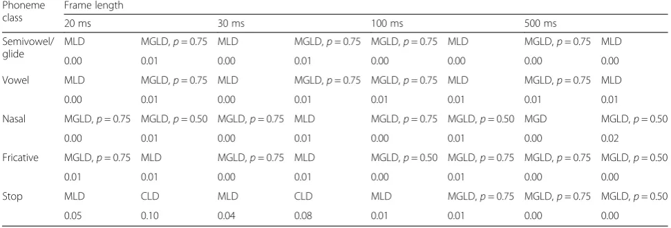
– The univariate Rayleigh distribution has been proposed for statistical univariate modeling of ADFT feature. Maybe as a consequence, it was expected that multivariate Rayleigh distribution (CRD) would be also superior in modeling multivariate

distribution of ADFT; however, the evaluation results proposed MGLD, CGD, or CGevD as the best-fitted candidates.

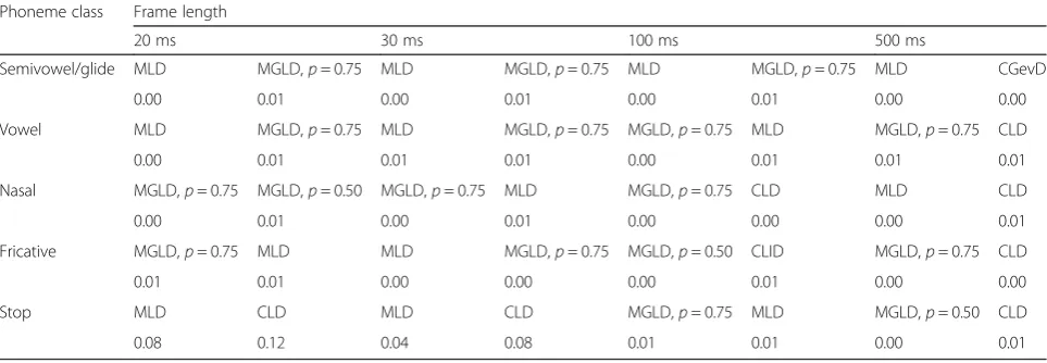
– The best-fitted candidate in the sense of the energy test for all phoneme classes in T, RDFT, IDFT, and DCT features with different frame lengths was either MLD or MGLD (withp∈{0.25, 0.50, 0.75}). In particular for frame lengths of 20 and 30 ms, which are mostly exploited in speech processing, either MLD or MGLD withp= 0.75 dominated. As a

Table 6Best-fitted multivariate distribution based on the energy test for LPC coefficients of five phoneme classes in different frame lengths

Phoneme class

Frame length

20 ms 30 ms 100 ms 500 ms

Semivowel/ glide

MGLD,p= 0.50 MGLD,p= 0.25 MGLD,p= 0.25 MGD MGLD,p= 0.25 MGLD,p= 0.50 MGD MGLD,p= 0.25

0.07 0.08 0.00 0.00 0.00 0.00 0.02 0.02

Vowel MGLD,p= 0.25 MGLD,p= 0.50 MGLD,p= 0.25 MGLD,p= 0.50 MGLD,p= 0.25 MGD MGLD,p= 0.25 MGD

0.01 0.01 0.01 0.01 0.01 0.01 0.00 0.00

Nasal MGLD,p= 0.25 MGD MGLD,p= 0.25 MGD MGD MGLD,p= 0.25 MGD MGLD,p= 0.25

0.00 0.00 0.00 0.00 0.00 0.01 0.00 0.00

Fricative MGLD,p= 0.25 MGD MGLD,p= 0.25 MGD MGLD,p= 0.25 MGLD,p= 0.50 MGD CLD

0.00 0.00 0.00 0.00 0.00 0.00 0.02 0.03

Stop MGLD,p= 0.25 MGLD,p= 0.25 MGLD,p= 0.25 MGLD,p= 0.50 MGLD,p= 0.25 MGD MGD MGLD,p= 0.25

0.02 0.02 0.01 0.01 0.00 0.00 0.00 0.00

Table 5Best-fitted multivariate distribution based on the energy test for ADFT coefficients of five phoneme classes in different frame lengths

Phoneme class

Frame length

20 ms 30 ms 100 ms 500 ms

Semivowel/ glide

MGLD,p= 0.75 MGLD,p= 0.50 MGLD,p= 0.75 MGLD,p= 0.50 MGLD,p= 0.50 MGLD,p= 0.25 CGevD CGD

0.05 0.06 0.03 0.04 0.02 0.02 0.00 0.01

Vowel MGLD,p= 0.75 MGLD,p= 0.50 MGLD,p= 0.75 MGLD,p= 0.50 CGevD MGLD,p= 0.75 MGLD,p= 0.50 MGLD,p= 0.25

0.04 0.05 0.04 0.05 0.03 0.04 0.02 0.02

Nasal MGLD,p= 0.50 CGevD MGLD,p= 0.50 MGLD,p= 0.75 MGLD,p= 0.25 MGD MGLD,p= 0.25 MGLD,p= 0.50

0.04 0.04 0.02 0.02 0.03 0.03 0.00 0.00

Fricative MGLD,p= 0.75 CGD MGLD,p= 0.50 MGLD,p= 0.25 MGLD,p= 0.50 MGLD,p= 0.25 MGD MGLD,p= 0.25

0.04 0.04 0.02 0.02 0.03 0.03 0.00 0.00

Stop CGD CGevD CGD CGevD MGLD,p= 0.50 MGLD,p= 0.75 MGLD,p= 0.25 MGLD,p= 0.50

consequence, the Laplace distribution contributes more compared to the Gaussian distribution in the statistical multivariate modeling of T, RDFT, IDFT, and DCT features with short frame lengths.

– The best-fitted candidates for different phoneme classes with LPC feature was mostly MGD or MGLD with p= 0.25. As a consequence, the Gaussian distribution contributed more in the statistical multivariate modeling of LPC feature compared to the Laplace distribution.

– As the first or second best-fitted candidates for different process domains of a phoneme class with a fixed frame length mostly varied between MLD and MGLD (withp∈{0.25, 0.50, 0.75}), the statistical modeling of phonemes with a mixture of Gaussian and Laplace distributions is proposed.

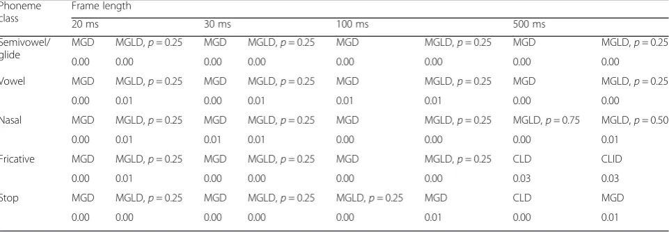
– The best-fitted candidate for most phoneme classes with MFCC features extracted from frames of length less than 500 ms is MGD, consistent with the

assumption of multivariate Gaussian distribution used in most speech recognition algorithms [2,3].

– The only copula-based distribution proposed by the energy test evaluation results was CGD for statistical modeling of the stop phoneme class in ADFT domain with frame lengths of 20 and 30 ms, and CGevD for semivowel/glide with frame length of 500 ms.

– Based on the evaluation results, in the sense of the energy test, the copula-based distributions using IFM method were mostly overcome by conventional distributions in the second experimental setup. As only one of parameter estimation methods of copula-based distribution, IFM method, was taken into account in the experimental evaluation, and the IFM method ends up a sub-optimal solution for parameter estimation, it is difficult to have a generic conclusion on copula-based distribution’s benefit in statistical modeling of speech frame. Table 7Best-fitted multivariate distribution based on the energy test for time coefficients of five phoneme classes in different frame lengths

Phoneme class

Frame length

20 ms 30 ms 100 ms 500 ms

Semivowel/ glide

MLD MGLD,p= 0.75 MLD MGLD,p= 0.75 MLD MGLD,p= 0.75 MGLD,p= 0.25 MGLD,p= 0.50

0.01 0.02 0.01 0.02 0.00 0.01 0.00 0.00

Vowel MLD MGLD,p= 0.75 MLD MGLD,p= 0.75 MLD MGLD,p= 0.75 MGLD,p= 0.75 MGLD,p= 0.50

0.01 0.02 0.00 0.02 0.00 0.01 0.00 0.01

Nasal MGLD,p= 0.75 MGLD,p= 0.50 MGLD,p= 0.75 MGLD,p= 0.50 MGLD,p= 0.50 MGLD,p= 0.50 MLD MGLD,p= 0.25

0.00 0.01 0.01 0.02 0.00 0.00 0.00 0.01

Fricative MLD MGLD,p= 0.75 MLD MGLD,p= 0.75 MLD MGLD,p= 0.75 MGLD,p= 0.25 MGLD,p= 0.50

0.00 0.01 0.00 0.01 0.00 0.00 0.00 0.00

Stop MLD CLD MLD CLD MGLD,p= 0.75 MLD MLD MGLD,p= 0.25

0.08 0.12 0.05 0.08 0.01 0.01 0.00 0.00

Table 8Best-fitted multivariate distribution based on the energy test for MFCC coefficients of five phoneme classes in different frame lengths

Phoneme class

Frame length

20 ms 30 ms 100 ms 500 ms

Semivowel/ glide

MGD MGLD,p= 0.25 MGD MGLD,p= 0.25 MGD MGLD,p= 0.25 MGD MGLD,p= 0.25

0.00 0.00 0.00 0.00 0.00 0.00 0.00 0.00

Vowel MGD MGLD,p= 0.25 MGD MGLD,p= 0.25 MGD MGLD,p= 0.25 MGD MGLD,p= 0.25

0.00 0.01 0.00 0.01 0.01 0.01 0.00 0.00

Nasal MGD MGLD,p= 0.25 MGD MGLD,p= 0.25 MGD MGLD,p= 0.25 MGLD,p= 0.75 MGLD,p= 0.50

0.00 0.01 0.01 0.01 0.00 0.00 0.00 0.01

Fricative MGD MGLD,p= 0.25 MGD MGLD,p= 0.25 MGD MGLD,p= 0.25 CLD CLID

0.00 0.01 0.00 0.00 0.00 0.00 0.03 0.03

Stop MGD MGLD,p= 0.25 MGD MGLD,p= 0.25 MGLD,p= 0.25 MGD CLD MGD

One of future work perspective might therefore be to study the power of statistical modeling of copula-based distribution of speech frame using optimal parameter estimation methods.

– In some cases, where the energy test values of the first and second best-fitted candidates are almost the same, there is almost no superiority in the sense of energy test between the first or sec-ond best-fitted distributions, e.g., the case of frica-tive phoneme in time domain with different frame lengths in Table 7.

6 Conclusions

In this paper, the multivariate distribution of speech features in various domains, e.g., time, DFT, DCT, MFCC, and LPC, was studied and a framework was proposed for exploring the best-fitted distribution among different candidates. Ten plausible candidates including five conventional distributions, e.g., the multi-variate Gaussian, multimulti-variate Laplace, and the mixture

of Gaussian–Laplace distributions (in three forms), and five copula-based distributions with marginal Laplace, independent marginal Laplace, Rayleigh, Gamma, and generalized extreme value (GEV) distributions were con-sidered to explore the effect of feature type, phoneme class (for English language), and frame length on the distribution.

The evaluation results of the test energy showed that the multivariate Laplace distribution statistically better models time and DFT features of speech signals compared to the multivariate Gaussian dis-tribution. For the amplitude of DFT features, the copula-based distribution with marginal Laplace dis-tribution was proposed as the best-fitted candidate. For the MFCC features, the best-fitted candidate was MGD, consistent with the assumption of multivariate Gaussian distribution used in most speech recogni-tion algorithms. For multivariate statistical modeling of different phoneme classes, the first or second best-fitted candidates for different domains (and also

Table 9Best-fitted multivariate distribution based on the energy test for RDFT coefficients of five phoneme classes in different frame lengths

Phoneme class

Frame length

20 ms 30 ms 100 ms 500 ms

Semivowel/ glide

MLD MGLD,p= 0.75 MLD MGLD,p= 0.75 MLD MGLD,p= 0.75 MGLD,p= 0.75 CLD

0.00 0.01 0.00 0.01 0.00 0.01 0.00 0.00

Vowel MLD MGLD,p= 0.75 MLD MGLD,p= 0.75 MLD MGLD,p= 0.75 MGLD,p= 0.75 MLD

0.00 0.01 0.00 0.01 0.00 0.00 0.00 0.00

Nasal MGLD,p= 0.75 MLD MGLD,p= 0.75 MGLD,p= 0.50 MGLD,p= 0.75 MGLD,p= 0.50 MGLD,p= 0.75 CGevD

0.00 0.01 0.00 0.01 0.00 0.00 0.01 0.01

Fricative MGLD,p= 0.75 MLD MGLD,p= 0.75 MLD MGLD,p= 0.75 MGLD,p= 0.50 MGLD,p= 0.50 MGD

0.01 0.01 0.00 0.01 0.00 0.00 0.00 0.00

Stop MLD CLID MLD CLD MGLD,p= 0.75 MLD MGLD,p= 0.25 MLD

0.06 0.10 0.04 0.08 0.01 0.01 0.00 0.00

Table 10Best-fitted multivariate distribution based on the energy test for IDFT coefficients of five phoneme classes in different frame lengths

Phoneme class Frame length

20 ms 30 ms 100 ms 500 ms

Semivowel/glide MLD MGLD,p= 0.75 MLD MGLD,p= 0.75 MLD MGLD,p= 0.75 MLD CGevD

0.00 0.01 0.00 0.01 0.00 0.01 0.00 0.00

Vowel MLD MGLD,p= 0.75 MLD MGLD,p= 0.75 MGLD,p= 0.75 MLD MGLD,p= 0.75 CLD

0.00 0.01 0.01 0.01 0.00 0.01 0.01 0.01

Nasal MGLD,p= 0.75 MGLD,p= 0.50 MGLD,p= 0.75 MLD MGLD,p= 0.75 CLD MLD CLD

0.00 0.01 0.00 0.01 0.00 0.00 0.00 0.01

Fricative MGLD,p= 0.75 MLD MLD MGLD,p= 0.75 MGLD,p= 0.50 CLID MGLD,p= 0.75 CLD

0.01 0.01 0.00 0.00 0.00 0.01 0.00 0.00

Stop MLD CLD MLD CLD MGLD,p= 0.75 MLD MGLD,p= 0.50 CLD

for different frame sizes) mostly varied between MLD and MGLD (with p∈{0.25, 0.50, 0.75}), i.e., a mixture of Gaussian and Laplace distributions. The future work of this study can lead toward the development of statistical speech processing algorithms exploiting Laplace, mixture of Laplace and Gaussian, or copula-based multivariate distribution, depending on the fea-ture type, phoneme class, and frame length.

Although the copula-based distribution was pro-posed as the best-fitted distribution for the modeling of amplitude of DFT, it is not the case for other features. It means that the copula-based approach requires more investigation in numbers of ways. First, the practical issues, e.g., the computational cost and the lack of sufficient amount of data for parameter estima-tion of some phoneme classes, e.g., stops, are needed to be considered. Second, as the IFM method used for parameter estimation of copula-based distribution ends up in a sub-optimal estimate, developing an optimal par-ameter estimation method for large vector dimensions is needed to have a fair evaluation of the copula-based distri-bution power in the statistical modeling of speech signals, e.g., compared to the optimal parameter estimation method used for MLD and MGD.

7 Appendix

The quantity ϕ, the energy, is defined as the difference between two pdfsfX0ð Þx andfX(x) by

ϕ¼1 2

Z Z

f xð Þ−f0ð Þx

f x′ −f0 x

′ _{R x ;x}′_dxdx′

¼1 2

Z Z

f xð Þf x′ þf₀ð Þxf₀ x′ −2f xð Þf₀ x′ R x ;x′dxdx′

ð28Þ

where the weight functionRis a monotonically decreas-ing function of Euclidian distance and the integrals

extend over the full variable space [44]. As the product of same distribution occurs in the first and second terms, it is not necessary to draw two different samples of the same pdf, and thereby, the first two terms can be neglected. The remaining third term has the form of expectation value of R and can be computed from the mean of all combinationsxN

i¼1¼fx1;…;xi;…;xNgfollowing

an unknown pdf f(x) and simulated Monte–Carlo sam-ples qN_j¼1¼fq1;…;qj;…;qMg following f0(x), thus the

energy statistic can be given by Eq. (29).

ϕNM¼ 1 N Nð −1Þ

X

t>i

Rxi_−xt

þ 1 M Mð −1Þ

X

j>n

R q n_−qj

− 1

NM

XN

i¼1

XM

j¼1

Rxi−qj

ð29Þ

It is noted that since the evaluation of ϕ requires a summation over integrals, which is typically difficult,f0is preferred to be represented by a set of samples generated through a Monte–Carlo simulation.

8 Additional file

Additional file 1:List of speakers and sentences from TIMIT dataset used in the evaluations.

Competing interests

The authors declare that they have no competing interests.

Authors’contributions

In this paper, AA and HV developed the concept and designed experiments. Also, AA and HV prepared the first draft of the paper. AA implemented the algorithms and did the simulations. HS supervised the project and edited the manuscript. The final design of copula-based technique and also analysis of the related experiments were done by ZM. HV and AA prepared the revisions of the paper, and ZM edited the revisions. All authors discussed the final

Table 11Best-fitted multivariate distribution based on the energy test for DCT coefficients of five phoneme classes in different frame lengths

Phoneme class

Frame length

20 ms 30 ms 100 ms 500 ms

Semivowel/ glide

MLD MGLD,p= 0.75 MLD MGLD,p= 0.75 MGLD,p= 0.75 MLD MGLD,p= 0.75 MLD

0.00 0.01 0.00 0.01 0.00 0.00 0.00 0.00

Vowel MLD MGLD,p= 0.75 MLD MGLD,p= 0.75 MGLD,p= 0.75 MLD MGLD,p= 0.75 MLD

0.00 0.01 0.00 0.01 0.01 0.01 0.01 0.01

Nasal MGLD,p= 0.75 MGLD,p= 0.50 MGLD,p= 0.75 MLD MGLD,p= 0.75 MGLD,p= 0.50 MGD MGLD,p= 0.50

0.00 0.01 0.00 0.01 0.00 0.01 0.00 0.02

Fricative MGLD,p= 0.75 MLD MGLD,p= 0.75 MLD MGLD,p= 0.50 MGLD,p= 0.75 MGLD,p= 0.75 MGLD,p= 0.50

0.01 0.01 0.00 0.01 0.00 0.01 0.00 0.00

Stop MLD CLD MLD CLD MLD MGLD,p= 0.75 MGLD,p= 0.75 MGLD,p= 0.50

results. HV is the corresponding author of the paper. All authors read and approved the final manuscript.

Author details

1_{Department of Medical Physics and Acoustics, University of Oldenburg,}

Oldenburg, Germany.2_{Faculty of New Sciences and Technologies, University} of Tehran, Tehran, Iran.3_{Department of Computer Engineering, Sharif} University of Technology, Tehran, Iran.4Department of Statistics, Shiraz University, Shiraz, Iran.

Received: 14 August 2014 Accepted: 29 November 2015

References

1. DY Zhao, Model based speech enhancement and coding, Ph.D., Royal Institute of Technology, KTH (2007)

2. L Rabiner, A tutorial on hidden Markov models and selected applications in speech recognition. Proc. IEEE77, 257–286 (1989)

3. Huang, X, Acero, A, and Hon, H-W, Spoken language processing: a guide to theory, algorithm, and system development, Prentice Hall PTR, 2001 4. H Zen, K Tokuda, AW Black, Statistical parametric speech synthesis. Speech

Comm.51, 1039–1064 (2009)

5. Z Xin, P Jancovic, L Ju, M Kokuer, Speech signal enhancement based on map algorithm in the ICA space. Signal Processing, IEEE Transactions on56, 1812–1820 (2008)

6. R Martin, Speech enhancement based on minimum mean-square error estimation and super-Gaussian priors. Speech and Audio Processing, IEEE Transactions on13, 845–856 (2005)

7. J-W Shin, J-H Chang, NS Kim, Statistical modeling of speech signals based on generalized Gamma distribution. Signal Processing Letters, IEEE12(3), 258_–261 (2005)

8. A Aroudi, H Veisi, and H Sameti, Hidden Markov Model-based Speech Enhancement Using Multivariate Laplace and Gaussian Distributions, IET Signal Processing,9(2), 177–185, 2015, (doi:10.1049/iet-spr.2014.0032) 9. H Veisi, H Sameti, Speech enhancement using hidden Markov models in

Mel-frequency domain. Speech Commun.55, 205_–220 (2013)

10. Y Ephraim, A Bayesian estimation approach for speech enhancement using hidden Markov models. Trans. Sig. Proc.40, 725–735 (1992)

11. Y Ephraim, D Malah, Speech enhancement using a minimum-mean square error short-time spectral amplitude estimator.

Acoustics, Speech and Signal Processing, IEEE Transactions on32, 1109–1121 (1984)

12. R McAulay, M Malpass, Speech enhancement using a soft-decision noise suppression filter. Acoustics, Speech and Signal Processing, IEEE Transactions on28, 137–145 (1980)

13. A Fazel, S Chakrabartty, An overview of statistical pattern recognition techniques for speaker verification. Circuits and Systems Magazine, IEEE11, 62–81 (2011)

14. S Gazor, Z Wei, Speech probability distribution. Signal Processing Letters, IEEE10, 204–207 (2003)

15. Allen, AO, Probability, statistics, and queueing theory with computer science applications, Academic Press, Inc., 1978

16. Papoulis, A, Probability, random variables and stochastic processes, McGraw-Hill Companies, 1991

17. B Chen, PC Loizou, A Laplacian-based MMSE estimator for speech enhancement. Speech Commun.49, 134–143 (2007)

18. JS Erkelens, J Jensen, R Heusdens, Speech enhancement based on rayleigh mixture modeling of speech spectral amplitude distributions, European Signal Proc. Conf. EUSIPCO, 2007

19. H Brehm, W Stammler, Description and generation of spherically invariant speech-model signals. Signal Process.12, 119–141 (1987)

20. JP LeBlanc, PL De Leon, Speech separation by kurtosis maximization, in

Acoustics, Speech and Signal Processing, 1998. Proceedings of the 1998 IEEE International Conference on, 1998

21. J Jensen, I Batina, RC Hendriks, R Heusdens, A study of the distribution of time-domain speech samples and discrete fourier coefficients, Proc. IEEE First BENELUX/DSP Valley Signal Processing Symposium, 2005 22. C Schölzel, P Friederichs, Multivariate non-normally distributed random

variables in climate research; introduction to the copula approach. Nonlin. Processes Geophys.15, 761–772 (2008)

23. T Ané, C Kharoubi, Dependence structure and risk measure. J. Bus.76, 411_–438 (2003)

24. JC Rodriguez, Measuring financial contagion: a copula approach. Journal of Empirical Finance14, 401–423 (2007)

25. C Genest, M Gendron, M Bourdeau-Brien, The advent of copulas in finance. European Journal of Finance15, 609_–618 (2009)

26. G Palombo, Multivariate goodness of fit procedures for unbinned data: an annotated bibliography,arXiv, 2011, 1102.2407v1.

27. AW Black, H Zen, K Tokuda, Statistical parametric speech synthesis, in

Acoustics, Speech and Signal Processing, 2007. ICASSP 2007. IEEE International Conference, 2007

28. S Srinivasan, J Samuelsson, WB Kleijn, Codebook-based Bayesian speech enhancement for nonstationary environments. Audio, Speech, and Language Processing, IEEE Transactions on15, 441_–452 (2007)

29. A Sklar, Fonctions de Répartition à n Dimensions et Leurs Marges. Publications Inst. Statist. Univ. Paris8, 229–231 (1959)

30. RB Nelsen,An introduction to copulas(Springer, New York, 2006) 31. E Bouye, VD, A Nikeghbali, G Riboulet, and T Roncalli,,_‘Copulas for

finance: a reading guide and some applications’, Working Paper. Groupe de Recherche Operationnelle, Credit Lyonnais, Available at http://ssrn.com/abstract=1032533, Nov. 2013.

32. Joe, H, Multivariate Models and Dependence Concepts, Chapman and Hall, 1997

33. W Hoeffding, Scale—invariant correlation theory, inThe Collected Works of Wassily Hoeffding, ed. by NI Fisher, PK Sen (Springer, New York, 1994) 34. P Embrechts, F Lindskog, and A McNeil,_‘Modelling Dependence with

Copulas and Applications to Risk Management’,Handbook of Heavy Tailed Distributions in Finance, Rachev, S. (ed), Elsevier, 329–38 2001

35. X Chen, Y Fan, Estimation of copula-based semiparametric time series models, Vanderbilt University Department of Economics, 2004. 36. G Biau, M Wegkamp, A note on minimum distance estimation of copula

densities. Statistics & Probability Letters73, 105–114 (2005) 37. BVM Mendes, EFL De Melo, RB Nelsen, Robust fits for copula models.

Communications in Statistics: Simulation and Computation36, 997_–1017 (2007) 38. Bowman, AW and Azzalini, A., Applied smoothing techniques for

data analysis: the kernel approach with S-plus illustrations, Clarendon Press, 1997

39. J Yan, Enjoy the joy of copulas: with a package copula. J. Stat. Softw.21, 1–21 (2007)

40. Bellman, R.E, Adaptive control processes: a guided tour, Princeton University Press, 1961

41. PJ Clark, FC Evans, Generalization of a nearest neighbor measure of dispersion for use in K dimensions. Ecology60, 316–317 (1979)

42. KV Mardia, Measures of multivariate skewness and kurtosis with applications. Biometrika57, 519–530 (1970)

43. JH Friedman, LC Rafsky, Multivariate generalizations of the Wald-Wolfowitz and Smirnov two-sample tests. Ann. Stat.7, 697–717 (1979)

44. B Aslan, G Zech, Statistical energy as a tool for binning-free, multivariate goodness-of-fit tests, two-sample comparison and unfolding. Nuclear Instruments and Methods in Physics Research, Section A: Accelerators, Spectrometers, Detectors and Associated Equipment537, 626–636 (2005) 45. V Schmidt, E James, Gentle: random number generation and Monte Carlo

methods. Metrika64, 251–252 (2006)

46. G Muraleedharan, C.G.S.a.C.L., Characteristic and Moment Generating Functions of Generalized Extreme Value Distribution,Sea Level Rise, Coastal Engineering, Shorelines and Tides, Nova Science Publishers, 269–276 2011. 47. Minka, TP,‘Estimating a Gamma distribution’, http://research.microsoft.com/

en-us/um/people/minka/papers/minka-gamma.pdf, Dec. 2012. 48. Paul Embrechts, CK, Thomas Mikosch, Modelling extremal events: for

insurance and finance, Springer, 1997

49. JC Lagarias, JA Reeds, MH Wright, PE Wright, Convergence properties of the Nelder_–Mead simplex method in low dimensions.

SIAM J. on Optimization9, 112–147 (1998)

50. K Fragiadakis, SG Meintanis, Goodness-of-fit tests for multivariate Laplace distributions. Math. Comput. Model.53, 769–779 (2011)

51. Garofolo, JS, Lamel, LF, Fisher, WM, Fiscus, JG, Pallett, DS, and Dahlgren, NL, Acoustic phonetic continuous speech corpus, NIST, 1993

52. Efron, B. and Tibshirani, R.J., An introduction to the Bootstrap, CRC press, 1994 53. B Aslan, and G Zech,A New Class of Binning Free, Multivariate Goodness-of-Fit