Adaptive Virtual Partitioning for OLAP Query Processing in
a Database Cluster
Alexandre A. B. Lima1, Marta Mattoso1, Patrick Valduriez2
1 Computer Science Department, COPPE, Federal University of Rio de Janeiro – Brazil
{assis, marta}@cos.ufrj.br 2 INRIA and LIRMM, Montpellier – France
Abstract. OLAP queries are typically heavy-weight and ad-hoc thus requiring high storage capacity and processing power. In this paper, we address this problem using a database cluster which we see as a cost-effective alternative to a tightly-coupled multiprocessor. We propose a solution to efficient OLAP query processing using a simple data parallel processing technique called adaptive virtual partitioning which dynamically tunes partition sizes, without requiring any knowledge about the database and the DBMS. To validate our solution, we implemented a Java prototype on a 32 node cluster system and ran experiments with typical queries of the TPC-H benchmark. The results show that our solution yields linear, and sometimes super-linear, speedup. In many cases, it outperforms traditional virtual partitioning by factors superior to 10.
Categories and Subject Descriptors: Information Systems [Miscellaneous]: Databases Keywords: Parallel Databases, Database Cluster, Query Processing
1. INTRODUCTION
On-Line Analytical Processing (OLAP) applications typically access large databases using heavy-weight read-intensive queries. Updates may occur but at specific predefined times. This is illustrated in the TPC-H Benchmark [TPC 2004], representative of OLAP systems. Out of twenty-four database queries, there are twenty-two complex heavy-weight read-only queries and two updates. Furthermore, OLAP queries have an ad-hoc nature. As users get more experienced about their OLAP systems, they demand more efficient ad-hoc query support [Gorla 2003].
The efficient execution of ad-hoc heavy-weight OLAP queries is still an open problem, mainly when efficiency means as fast as possible. Traditionally, high-performance of database management has been achieved with parallel database systems [Valduriez 1993], using tightly-coupled multiprocessors and data partitioning and replication techniques. Although quite effective, this solution requires the database system to have full control over the data and is expensive in terms of hardware and software. Clusters of PC servers appear as a cost-effective alternative. Recently, the database cluster ap-proach has gained much interest for various database applications ([Akal et al. 2002], [Gançarski et al. 2002], and [Röhm et al. 2000]). A database cluster [Akal et al. 2002] is a set of PC servers intercon-nected by a dedicated high-speed network, each one having its own processor(s) and hard disk(s), and running an off-the-shelf DBMS. Similar to multiprocessors, various cluster system architectures are possible: shared-disk, shared-cache and shared-nothing [Özsu and Valduriez 1999]. Shared-nothing (or distributed memory) is the only architecture that does not incur the additional cost of a special interconnect. Furthermore, shared-nothing can scale up to very large configurations. In this paper,
Work partially funded by CNPq, CAPES, INRIA and COFECUB.
we strive to exploit a shared-nothing architecture as in PowerDB [Schek et al. 2000] and Leg@Net [Gançarski et al. 2002]. Each cluster node can simply run an inexpensive (non parallel) DBMS. In our case, we use the PostgreSQL [PostgreSQL 2004] DBMS, which is freeware. Furthermore, the DBMS is used as a "black-box" component [Gançarski et al. 2002]. In other words, its source code is not available and cannot be changed or extended to be "cluster-aware". Therefore, extra functionality like parallel query processing capabilities must be implemented via middleware.
OLAP query processing in a database cluster is addressed in [Akal et al. 2002]. The approach which we refer to as simple virtual partitioning (SVP) consists in fully replicating a database along a set of sites, and breaking each query in sub-queries by adding predicates. Each DBMS receives a sub-query and is forced to process a different subset of data items. Each subset is called a virtual partition. Such strategy allows for greater flexibility on node allocation for query processing than physical (static) data partitioning [Özsu and Valduriez 1999]. A preventive replication protocol [Coulon et al. 2004], which scales up well in cluster systems, could be used to keep copy consistency. However, SVP presents some problems. First, determining the best virtual partitioning attributes and value ranges can be a complex task since assuming uniform value distribution is not very realistic [Akal et al. 2002]. Second, some DBMSs perform full table scans instead of indexed access when retrieving tuples from large intervals of values. This reduces the benefits of parallel disk access since one node could incidentally read all pages of a virtually partitioned table. It makes SVP more dependent on the underlying DBMS query capabilities. Third, as a query cannot be externally modified while being executed, load balancing is difficult to achieve and depends on the good initial partition design.
To overcome these problems, we proposed fine-grained virtual partitioning (FGVP) [Lima et al. 2004]. As SVP, FGVP employs sub-queries to obtain virtual partitions. Unlike SVP, FGVP uses a large number of sub-queries instead of one per DBMS. Working with small, light-weight sub-queries avoids full table scans and makes query processing less vulnerable to DBMS idiosyncrasies. Our preliminary experimental results showed that FGVP outperforms SVP for some representative OLAP queries. However, we used a simplistic method for partition size determination, based on database statistics and query processing time estimates. In practice, these estimates are hard to obtain with black-box DBMSs which makes it difficult to build a DBMS-independent cluster query processor.
In this paper, we address the partition size determination problem by using an adaptive approach that dynamically tunes partition sizes. We proposeadaptive virtual partitioning(AVP) which is
com-pletely DBMS-independent and uses neither database statistics nor query processing time estimates. AVP avoids full table scans on huge database tables in addition to parallel processing. It is also easy to implement. To validate our approach, we implemented AVP in a Java prototype and ran experiments on a 32-node cluster running PostgreSQL. The results show that linear and sometimes super-linear speedup is obtained for many tested OLAP queries. In the worst cases, almost linear speedup is achieved, which is excellent considering the simplicity of the techniques. AVP also shows much better performance than SVP in most cases. In all cases, it is more robust.
This paper is organized as follows. Section 2 introduces the general principle of simple virtual partitioning and describes our adaptive algorithm for dynamic determination and tuning of parti-tion sizes. Secparti-tion 3 describes our query processor architecture. Secparti-tion 4 describes our prototype implementation and our experimental results. Section 5 concludes.
2. ADAPTIVE VIRTUAL PARTITIONING
2.1 SVP and FGVP
The goal of Simple Virtual Partitioning (SVP) [Akal et al. 2002] is to achieve intra-query parallelism in OLAP query processing. Considering a database cluster with full database replication over all cluster nodes, SVP limits the amount of data processed by each DBMS by adding predicates to incoming queries. Doing so, it forces each DBMS to process a different subset of data items. For example, let us consider query Q6, taken from TPC-H Benchmark [TPC 2004], which accesses its largest fact table (Lineitem):
Q6: select sum(l_extendedprice * l_discount) as revenue from Lineitem
where l_shipdate≥date ’1994-01-01’
and l_shipdate<date ’1994-01-01’ + interval ’1 year’ and l_discount between .06 - 0.01 and .06 + 0.01 and l_quantity<24;
Q6 is a typical OLAP query. It has an aggregation function and accesses a huge table (in TPC-H smallest configuration, Lineitem has 6,001,215 tuples). For simplicity, we chose a query that contains no joins. Using SVP, this query would typically be rewritten by adding the predicate “and l_orderkey
≥:v1 and l_orderkey<:v2” to the “where” clause of Q6. The rewritten query can then be submitted to the nodes that participate on Q6 processing. Lineitem’s primary key is formed by the attributes l_orderkey and l_linenumber. Since there is a clustered index on the primary key and l_orderkey has a large range of values, l_orderkey has been chosen as the virtual partitioning attribute. Each node receives the same query, but with different values for v1 and v2, so that the whole range of l_orderkey is scanned. This technique allows great flexibility for node allocation during query processing: any set of nodes in the cluster can be chosen for executing any query.
Simplicity is one of SVP most appealing characteristics. However, its efficiency depends on some factors. First of all, there must be a clustered index associated to the partitioning attribute. Making each cluster node to process a different subset of tuples does not guarantee that only a subset of the disk pages associated to the partitioned table will be read by each node. Occasionally, one node could read all of them. If tuples are physically ordered according to the partitioning attribute, full-table reading can be avoided if a clustered index is available.
Having a clustered index is necessary but it is not enough. The clustered index must be used by the underlying DBMSs during sub-query processing. Some DBMSs do not use indexes to access a table if they estimate that the number of accessed tuples is greater than some threshold. In this case, they perform a full table scan, which hurts the basic goal of SVP.
Uniform value distribution on the partitioning attribute is another requirement for SVP good perfor-mance. SVP is a static decomposition technique, requiring partition limits determined before query execution. Once submitted, sub-queries cannot be dynamically changed when black-box DBMSs are employed. Such characteristic prevents a cluster query processor from performing dynamic load balancing among cluster nodes since task reassignment cannot be done. In order to avoid load unbal-ancing, one approach could be to consider information concerning value distribution during virtual partition size determination, at the very beginning of the process.
accessed tuples. Thus, our proposal was to have an initial number of virtual partitions greater than the number of participating nodes which is the main difference with SVP. Instead of one (possibly) heavy-weight query, FGVP makes each cluster node to process a set of small, light-weight sub-queries. These sub-queries are produced in the same way as SVP does: through query predicate addition.
Some advantages can be immediately obtained from the FGVP approach. First, if sub-queries are small enough, i.e., if they access small amounts of partitioned table data, DBMSs will effectively use clustered indexes, thus avoiding full table scans. This makes our technique more robust, as it is less vulnerable to the underlying DBMS idiosyncrasies. When considering join queries, FGVP can also be more attractive than SVP. Some join processing techniques, like hash-join and merge-join [Graefe 1993], require temporary disk-based structures when processing data that do not fit in main memory. Using small sub-queries, such structures are no longer necessary since only small amounts of data need to be processed by each sub-query at a time. In addition, having many sub-queries allows for dynamic load balancing. At the beginning of query processing, FGVP assigns each node a different virtual partition. Each node processes its partition through many sub-queries. If node N1 finishes before node N2, some non-processed N2 sub-queries can be re-assigned to N1.
Of course, some problems can arise. The most obvious problem concerns the size of each virtual partition. Such size is directly related to the number of sub-queries. The smaller the virtual partitions are, the more sub-queries we have. Having many sub-queries can degrade performance, especially if many non-partitioned tables are accessed. In [Lima et al. 2004], we adopted a simplistic method based on database statistics and query processing time estimates. Such estimates are very hard to obtain from black-box DBMSs. It makes it difficult the task of constructing a cluster query processor that should perform well no matter the DBMS being used.
2.2 AVP
One of the fundamental issues in FGVP is how to determine virtual partition sizes, i.e., how to find out value intervals to be used by each sub-query. The total processing cost of a query is determined by a number of components [Özsu and Valduriez 1999]. Before starting accessing data, there is the cost incurred by the generation of a query execution plan (QEP) for query parsing, translation and optimization. Then there is the query processing initialization cost, e.g. memory allocation and temporary data structures creation. After initialization, data can be read and the query processed. When there are no more data to process, the results must be sent to the requester and the system resources released. These are roughly the query processing phases.
The amount of data accessed by a query does not affect these phases in the same way. The time required for QEP generation for example is much more related to the query statement complexity than to the number of bytes read from disk. On the other hand, resource releasing can be more or less expensive depending on the amount of data processed and operations performed. How does this affect FGVP? If we work with too many small sub-queries, operations whose costs are not affected by the number of processed tuples (like QEP generation) will predominate and we will obtain poor performance. On the other hand, a small number of large queries could yield all the aforementioned problems (full table scans on the partitioned table, temporary disk-based structures, etc.). These problems could be even worse for FGVP than for SVP due to the greater number of sub-queries the former demands.
access structures and which algorithms would be effectively employed during query execution. We would have to guess some things and expect these “guessings” to be correct. Besides, for all such effort to be valid, we should try to answer the following questions: “Is there a ‘best’ size that should be used for all sub-queries during one query execution? If there is, what is the cost of finding it?”
Instead of addressing all these issues, we opted for a simpler, more dynamic approach which led to AVP. The AVP algorithm runs independently in each participating cluster node, avoiding inter-node communication (for partition size determination). At the beginning, each node receives an interval of values to work with. These intervals are determined exactly as for SVP. Then, each node performs the following steps:
(1) Start with a very small partition size beginning with the first key value of the received interval; (2) Execute a sub-query with this interval;
(3) Increase the partition size and execute the corresponding sub-query while the increase in execution time is proportionally smaller than the increase in partition size;
(4) Stop increasing. A stable size has been found;
(5) Monitor query execution time to detect performance deterioration;
(6) If deterioration is confirmed, i.e., there were consecutive worse executions, decrease size and return to Step 2.
These main steps of the algorithm illustrate some of our basic principles. Starting with a very small partition size avoids full table scans at the very beginning of the process. Otherwise, we would have to know the threshold after which the DBMS does not use clustered indexes and starts performing full table scans. Such information would have to be given by the database administrator.
When we increase partition size, we monitor query execution time. This allows us to determine after which point the query processing phases that are data-size independent do not influence too much total query execution time. If, for example, we double the partition size and we get an execution time that is almost twice the previous one, we have found such point. Thus we stop increasing the size.
System performance can deteriorate due to DBMS data cache misses and/or overall system load increase. It may happen that the size being used is too large and has benefited from previous data cache hits. In this case, it may be better to shrink partition size. That is precisely what step 6 does. It gives a chance to go back and inspect smaller partition sizes. On the other hand, if performance deterioration was due to a casual and temporary increase on system load or to data cache misses, keeping a small partition size can lead to poor performance. To avoid such situation, we go back to step 2 and restart increasing sizes.
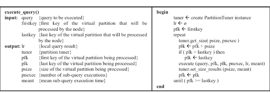
The general algorithm for query execution is shown in Figure 1. In our architecture, sub-query execution is performed by a Query Executor component (which executes the algorithm in Figure 1) and partition size determination and tuning is performed by a component called Partition Tuner. As Figure 1 shows, Query Executor and Partition Tuner interact to implement AVP. Basically, the Query Executor demands a partition size to the Partition Tuner; executes one or more sub-queries according to its instructions; and gives it feedback. This process restarts until the entire node assigned interval has been processed.
Fig. 1. Algorithm for sub-query execution.
the Partition Tuner goes to the “restarting” state. The partition size is decreased and the Partition Tuner goes back to “searching” state to restart size increasing.
In some states, the Partition Tuner determines that more than one sub-query will be executed with the same partition size. This is to try to diminish temporary system load influence when evaluating partition sizes performance. In such cases, the considered execution time is in fact the mean sub-query execution time. Avoiding potential system load fluctuations is also the goal of the performance deterioration verification carried on when the Partition Tuner is in “tuned” state.
In [Stöhr et al. 2000], small database partitions are also used for OLAP query processing with good results. The parallel architecture employed was shared-disk [Özsu and Valduriez 1999] but the authors claim that their technique can easily be used in other architectures. A data fragmentation technique is proposed, called multi-dimensional hierarchical fragmentation (MDHF). MDHF physically fragments the fact table. Its success solely depends on a good fragmentation. Fragmentation guidelines are given in [Stöhr et al. 2000]. Some depend on the query profile while others depend on the system, e.g. main memory or disk storage space. AVP does not depend on any of these factors. Partition sizes are obtained according to the dynamic query behavior. With respect to the architecture, as AVP is being used in a shared-nothing context with fully replicated databases, it can be directly used in shared-disk architectures.
3. QUERY PROCESSOR ARCHITECTURE
In this section, we show how query processing is carried out in our architecture. Figure 2 illustrates the global process.
Query processing starts when the Client Proxy receives a query from a client application. The query is then passed on to the Cluster Query Processor (CQP). CQP creates a new object, named Global Query Task (GQT), in a separate thread, to deal with the new query. GQT gets metadata from the Catalog and, with such information, determines the partitioning attributes. OLAP queries usually have aggregation and/or duplicate tuple elimination operations. Virtual partitioning requires extra steps after sub-queries completion in order to produce correct final results. In our architecture, the Global Result Collector (GRC) is responsible for such steps at a global level. GQT creates a new GRC in a separate thread. Afterwards, GQT sends the QEP to the Node Query Processor (NQP) of each participating node.
Fig. 2. Query processing - global components.
Fig. 3. Query processing - node components.
sends the response to the appropriate client application.
We now describe what happens at each cluster node during query processing. Figure 3 illustrates the main node components and their interaction. The main components that run in each cluster node are the Node Query Processor (NQP), the DBGateway (DBG) and the DBMS instance with the local database. When NQP receives a QEP, it creates a Local Query Task (LQT) object in a separate thread. LQT is responsible for one client query execution. Each different QEP received will generate a different LQT object. The QEP is sent to LQT, which creates a PartitionTuner object and, in a different thread, a Local Result Collector (LRC) object. Our goal with LRC creation is to avoid an occasional bottleneck that could appear in our architecture if all intermediate query results were directly sent to Global Result Collector. So, LRC performs the same tasks as Global Result Collector but in a node level. Afterwards, LQT creates a Query Executor (QE), also in a different execution thread. The QE role is to prepare final SQL queries that will be submitted by DBGateway to the DBMS. During query processing, QE communicates with PartitionTuner, which dynamically calculates and adjusts partition sizes using the adaptive algorithm proposed on section 2. Their interaction implements AVP. When QE is created, LQT gives it a range of keys to work with and a parameterized query. Then, each QE starts submitting SQL queries to DBGateway, each one corresponding to a different virtual partition.
repeated until there are no more virtual partitions to be processed. Then, QE sends LQT a message indicating its work is done. Afterwards, LQT receives the final local result from LRC and sends it to NQP. NQP takes two actions: sends the result to Global Result Collector and notifies Global Query Task that its work is finished.
In the next section, we give implementation details of our prototype. We also describe some exper-imental results.
4. EXPERIMENTAL VALIDATION
To validate our solution, we implemented a prototype on a cluster system and ran experiments with the TPC-H benchmark. In this section, we first present our prototype implementation and the exper-imental setup. Then we discuss the queries used in our experiments and the partitioning strategies for these queries. Finally, we report on speedup experiments for AVP and performance comparisons with SVP.
4.1 Experimental Setup
Our cluster system has 32 nodes, each with 2 Intel Xeon 2.4 GHz processors, 1 GB main memory, and a disk capacity of 20 GB. We use the PostgreSQL 7.3.4 DBMS running on Linux. We used the TPC Benchmark H because it is a decision support benchmark that “consists of a suite of business orientedad-hoc queries” [TPC 2004]. We generated the TPC-H database as specified in [TPC 2004],
using a scale factor of 5 which produced a database of approximately 11 GB. The fact tables (Orders and Lineitem) have clustered indexes on their primary keys. We also built indexes for all foreign keys of all fact and dimension tables. After data generation and indexes creation, database statistics were updated in order to be used by DBMS query optimizer. As our goal is to deal with ad-hoc queries,
no other optimization was performed. The database is replicated at each cluster node.
Our prototype is implemented in Java. Some components are implemented as Java RMI objects: Cluster- and NodeQueryProcessor, DBGateway, Global- and LocalQueryTask, Global- and LocalRe-sultComposer. Our implementation uses multi-threading. Each instance of Global- and LocalQuery-Task, Global- and LocalResultComposer and QueryExecutor runs in a different execution thread. Result composition is done in parallel at each node. Only the final global result composition is done by GRC in one of the participating nodes. To maximize system throughput and avoid bottlenecks, sub-query submission and result composition are processed by separate threads.
4.2 TPC-H Queries
To help understanding queries, we give a brief description of the TPC-H database structure. Eight tables are defined: six dimensions (Region, Nation, Supplier, Part, Customer and Partsupp) and two fact tables (Orders and Lineitem). Region and Nation are very small dimensions with 5 and 25 tuples respectively. This number is fixed and independent of the scale factor used for database generation. Let SF be the scale factor, the cardinalities of the other tables are: |Supplier|=SF*10,000;
|Customer|= SF*150,000; |Part|= SF*200,000; |Partsupp|= SF*800,000; |Orders|= SF*1,500,000; and |Lineitem| = SF*6,000,000. Lineitem is the largest table, followed by Orders, with 25% of its size. Lineitem tuples reference Orders tuples through a foreign key (l_orderkey) that is also part of its primary key.
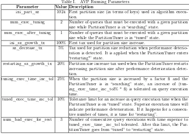
Table I. AVP Running Parameters
Parameter Value Description
ini_part_sz 1024 First partition size (in terms of keys) used in algorithm execu-tion.
num_exec_tuning 2 Number of queries that must be executed with a given partition size while PartitionTuner is in “searching” state.
num_exec_after_tuning 1 Number of queries that must be executed with a given partition size while the PartitionTuner is in “tuned” state.
ini_sz_growth_tx 100% First tax used for partition size increase.
sz_decrease_tx 5% Tax used for partition size reduction when performance deterio-ration is detected. It is applied when the PartitionTuner enters “restarting"’ state.
restarting_sz_growth_tx 20% Partition size increase tax used when the PartitionTuner restarts increasing partition size after performance deterioration detec-tion.
tuning_exec_time_inc_tol 25% When the partition size is increased by a factor fi and the PartitionTuner is in “searching” state, an increase of (tun-ing_exec_time_inc_tol% * fi) is tolerated on query execution time.
tuned_exec_time_inc_tol 10% Tolerance limit for an increase in query execution time when the PartitionTuner is on “tuned” state. Superior execution times will indicate performance deterioration. If it happens for a consecu-tive number of times, it is time for “restarting”.
num_bad_exec_for_rest 3 Number of consecutive query executions with time superior to tuned_exec_time_inc_tol tolerated. After this limit, the Par-titionTuner goes from “tuned” to “restarting” state.
aggregate operation and its “where” predicate is more selective, retrieving only 1.9% of tuples. Q14 joins Lineitem and Part. Q18 joins one dimension (Customer) and the two fact tables. Its main characteristic is that it also contains one sub-query on Lineitem table. This sub-query performs an aggregation and has no predicate to restrict Lineitem tuples being processed. Thus, these five queries were chosen because we believe they are quite representative of OLAP applications.
The virtual partitioning strategy employed is similar to that in [Akal et al. 2002]. For Q1 and Q6, it is based on l_orderkey since it is the first primary key attribute of Lineitem and has few tuples for each value. For Q5 and Q18, we use primary virtual fragmentation for the Orders table based on primary key o_orderkey and derived virtual fragmentation for the Lineitem table based on foreign key l_orderkey. For Q18, we also add a virtual fragmentation predicate to the sub-query as it does not affect query results. For Q14 we employ the same strategy as for Q1 and Q6, leaving the Part table not fragmented.
4.3 Speedup Experiments with AVP
We now describe results of experiments performed to analyze the speedup characteristics of AVP. Queries were executed using different numbers of nodes. Each one was run several times. Our graphics show mean query execution times. The AVP implementation uses some running parameters. Table I gives a brief description of each one and shows the values we used during our experiments.
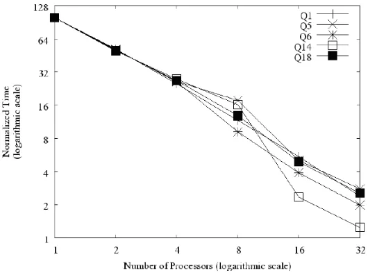
Fig. 4. Query execution times with AVP.
except for the very small tables Region and Nation on query Q5. Furthermore, all joins were processed through indexed nested-loop join algorithm [Graefe 1993], which needs no temporary disk structures. Merge- and hash-join algorithms, which may need such structures [Graefe 1993], were not employed in spite of being available. As the amount of data processed by each sub-query is small, some sort operations could be processed using main memory structures. This shows AVP efficacy in keeping sub-queries as fast as possible, avoiding extra disk access.
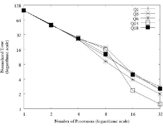
The results from our experiments are shown in Figure 4. We show normalized mean query execution times for an increasing number of nodes. Times were normalized by dividing each mean response time by the greatest mean response time of its associated query. In order to ease reading and analysis, we use logarithmic scales.
One characteristic of AVP is that partition sizes used by sub-queries are independent of interval sizes assigned to nodes at the beginning of the process. Thus, we expect that large intervals will require more sub-queries than small ones. As stated before, some query processing operations (parsing and optimization, for example) are not impacted by virtual partitioning. So, having many sub-queries is expected to reduce the overall AVP performance. This explains why all queries present sub-linear speedup with 2 and 4 nodes (in spite of being very close to linear speedup).
With 8 processors, queries Q1 and Q6 start having super-linear speedup. This is due to the reduction in the number of sub-queries and to the fact that they access only the virtually partitioned table Lineitem. Q18 has execution time only 6.9% higher than the expected time (in absolute terms, 0.98 seconds) because it accesses a non-partitioned dimension table (Customer). Even then the speedup is very good because the query time is dominated by sub-query processing, which accesses a partitioned table (Lineitem). The worst speedups for this configuration are for queries Q5 and Q14. Both access non-partitioned tables and the large number of sub-queries hurts AVP performance. For 16 and 32 nodes all queries have super-linear speedup. As fewer sub-queries are processed by each node in these configurations, the effect of partition size-independent operations and of accessing non-partitioned tables is negligible.
4.4 AVP versus SVP
Fig. 5. SVP versus AVP.
from 1 to 32, plotted in logarithmic scale. To explain the figure, we analyzed execution plans generated by PostgreSQL for each query. First, we analyzed execution plans for ordinary sequential execution, i.e., executions with one node and no virtual partitioning. Then, we analyzed execution plans for virtually partitioned queries with different partition sizes. It facilitates understanding how and when virtual partitioning influences QEP generation.
For the sequential execution of query Q1, PostgreSQL generates a plan that performs a full table scan on Lineitem. The retrieved tuples are then sorted for grouping. As Q1 presents a “where” predicate which is not very selective, such sorting operation is very expensive. Sub-queries generated by SVP in all cases (from 1 to 32 nodes) have partition sizes that are not small enough to avoid full table scans. Also, from 1 to 4 nodes the number of tuples retrieved is high, thereby requiring expensive sorting. From 8 to 32 nodes, sorting is not so expensive. As AVP sub-queries require neither full table scans nor expensive sorting, Q1 presents better performance with AVP than with SVP in all configurations. With 32 nodes, AVP performs 6.36 times better than SVP.
The sequential execution plan for Q5 shows sequential scans for accessing all tables. This is the same plan generated when SVP is used with only 1 node. With 2 and 4 nodes, the partitioning strategy starts being effective and the fact tables are accessed through clustered indexes. In fact, we noticed that the predicate added for derived partitioning (on the Lineitem table) has no practical effect. This is because Lineitem is joined to Orders through an indexed nested-loop algorithm. All other tables are fully scanned. This explains why AVP presents better performance than SVP with 1, 2 and 4 nodes. With 8 nodes, the Supplier table is accessed through an index and this is the case for almost all tables with 16 and 32 nodes (the exceptions are the very small dimensions Region and Nation). These executions with no full scans together with the fact that with SVP only one sub-query is processed by each node, explain the good performance of SVP relative to AVP. With 32 nodes, SVP outperforms AVP by a factor of 1.84. But the worst case is with 8 nodes when SVP outperforms AVP by a factor of 5.41 which is due to the high number of queries with AVP.
aggregation functions explains it. In all other configurations (2 to 32 nodes), AVP outperforms SVP. With 32 nodes, AVP is 28.72 times faster than SVP.
The sequential QEP for query Q14 also shows full table scan operations for retrieving tuples from both tables (Lineitem and Part). SVP sub-queries for 1, 2, 4 and 8 nodes are processed in the same way. With 16 and 32 nodes, the Part table is accessed through an index but the Lineitem table keeps being fully scanned. The predicate added for partitioning has only a marginal effect on overall query processing as it allows this indexed access to Part table. Due to the high number of sub-queries associated to the access to a non-partitioned table, SVP outperforms AVP with 1 and 2 nodes by a factor of 3.09 and 1.56, respectively. However, from 4 to 32 nodes, AVP outperforms SVP. From Figure 5, we see that this difference rises very sharply when we go from 8 to 16 nodes. It goes from 2.06 to 11.60. And it almost doubles when we go from 16 to 32 nodes (22.10). The reason is the use of a merge-join algorithm, which requires a sort operation on Lineitem tuples. As, with AVP, the tables are joined through an indexed nested-loop, the performance differences become very high.
Query Q18 is evaluated in a very inefficient way by PostgreSQL. Looking at the query statement, we see that its sub-query result is constant and does not depend on the tuples being processed in the outer query. It could be evaluated once at the beginning of query processing and joined to outer tuples as they were being produced. But this is not what happens. In fact, the QEP shows that the sub-query is re-evaluated for each outer tuple. The outer query has a join among the Customer, Orders and Lineitem tables and no restrictive predicates. This means that the sub-query is re-evaluated for each tuple in the Orders fact table. Besides, all the tables are fully scanned. This explains why this query takes a very long time to execute. The partitioning strategy includes a predicate on the sub-query. AVP outperforms SVP for Q18 in all configurations by factors that vary from 4.22 (with 2 nodes) to 36.68 (with 1 node). The curve associated to Q18 shows very interesting characteristics. First, we can notice a sharp decrease from 1 to 2 nodes. This is due to the fact that the query generated by SVP for execution with 1 node performs a full scan on the Orders table while for 2 nodes the clustered index is used, yielding a reduction of 50% on the number of sub-query executions. So, SVP shows a good performance improvement. Another interesting characteristic is that the curve decreases when we go from 16 to 32 nodes. In this case, the factor drops from 18.89 to 16.85. This is also due to the reduction in the number of Orders tuples being processed. It is important to say that the derived partitioning of Lineitem is only effective with 16 and 32 nodes for SVP. With less than 16 nodes, the Lineitem table is always fully scanned. On the other hand, for SVP, the predicate added to the sub-query never avoids full table scans. For AVP, no table scans are performed in any case.
In general, the results obtained for SVP in our experiments were very different from those shown in [Akal et al. 2002]. In that work, another DBMS was employed. We believe that this explains the differences observed. With PostgreSQL, SVP showed poor performance in the majority of cases. On the other hand, AVP performed very well, appearing to be more robust.
We did not experience problems related to load unbalancing among cluster nodes. This is due to TPC-H value distribution for partitioning attributes. Roughly, all nodes had to process the same amount of data. It does not affect our results in the sense that the same data and partitioning criteria were used for SVP experiments.
5. CONCLUSION
easy to implement.
To validate our solution, we implemented AVP in a 32-node database cluster that has a shared-nothing cluster architecture to provide for scale up to large configurations. It supports black-box DBMSs using non intrusive, simple techniques implemented by Java middleware. Thus, it can support any kind of relational DBMS. We ran experiments with typical queries of the TPC-H benchmark. The results show that in many cases AVP yields linear and super-linear speedup. Experiments with 16 and 32 cluster nodes showed super-linear speedup for all tested queries, in spite of their different characteristics. This is a very desirable behavior for a technique implemented on top of a highly scalable shared-nothing architecture.
Our experiments also compared AVP and SVP performances. In many cases, AVP outperforms SVP by factors superior to 10 (28, in the best case). By analyzing query execution plans generated by PostgreSQL, we noticed that AVP sub-queries are not influenced by the number of cluster nodes used for query processing. Thus, it can provide for consistent improvement in query processing in small and large cluster configurations. On the other hand, execution plans associated to SVP sub-queries are very different when considering the number of cluster nodes. It happens because with SVP the amount of data processed by each sub-query is directly proportional to the number of nodes employed. AVP proved to be very robust since it is extremely efficient for heavy-weight queries and yields good performance for light-weight queries with small and large cluster configurations.
6. ACKNOWLEDGEMENTS
Alexandre A. B. Lima would like to thank CAPES and Unigranrio University for their support while visiting the University of Nantes during his doctoral studies.
REFERENCES
Akal, F.,Böhm, K.,and Schek, H.-J.Olap query evaluation in a database cluster: A performance study on intra-query parallelism. InProceedings of the 6th East European Conference on Advances in Databases and Information Systems. London, UK, pp. 218–231, 2002.
Coulon, C.,Pacitti, E.,and Valduriez, P. Scaling up the preventive replication of autonomous databases in cluster systems. InProceedings of the International Conference on High Performance Computing for Computational Science. Valencia, Spain, pp. 170–183, 2004.
Gançarski, S.,Naacke, H.,Pacitti, E.,and Valduriez, P. Parallel processing with autonomous databases in a cluster system. InProceedings of the Confederated International Conferences DOA, CoopIS and ODBASE. Springer-Verlag, London, UK, pp. 410–428, 2002.
Gorla, N. Features to consider in a data warehousing system. Commun. ACM 46 (11): 111–115, 2003.
Graefe, G. Query evaluation techniques for large databases. ACM Comput. Surv.25 (2): 73–169, 1993.
Lima, A. A. B.,Mattoso, M.,and Valduriez, P. Olap query processing in a database cluster. InProceedings of the International Euro-Par Conference on Parallel Processing. pp. 355–362, 2004.
Özsu, T. M. and Valduriez, P.Principles of Distributed Database Systems (2nd Edition). Prentice Hall, 1999.
PostgreSQL. http://www.postgres.org, 2004.
Röhm, U.,Böhm, K.,and Schek, H.-J.Olap query routing and physical design in a database cluster. InProceedings of the 7th International Conference on Extending Database Technology. London, UK, pp. 254–268, 2000.
Schek, H.-J.,Bohm, K.,Grabs, T.,Rohm, U.,Schuldt, H.,and Weber, R. Hyperdatabases. InProceedings of the First International Conference on Web Information Systems Engineering. Hong Kong, China, pp. 14–23, 2000.
Stöhr, T.,Märtens, H.,and Rahm, E. Multi-dimensional database allocation for parallel data warehouses. In
Proceedings of the 26th International Conference on Very Large Data Bases. Cairo, Egypt, pp. 273–284, 2000.
TPC. TPC Benchmark H (Decision Support).http://www.tpc.org/tpch, 2004.