Parallelizing Spectrally Regularized Kernel Algorithms
Nicole M¨ucke [email protected]
Institute of Stochastics and Applications, University of Stuttgart Pfaffenwaldring 57
70569 Stuttgart, Germany
Gilles Blanchard∗ [email protected]
Institute of Mathematics, University of Potsdam Karl-Liebknecht-Strae 24-25
14476 Potsdam, Germany
Editor:Ingo Steinwart
Abstract
We consider a distributed learning approach in supervised learning for a large class of spec-tral regularization methods in an reproducing kernel Hilbert space (RKHS) framework. The data set of size n is partitioned into m = O(nα), α < 1
2, disjoint subsamples. On
each subsample, some spectral regularization method (belonging to a large class, includ-ing in particular Kernel Ridge Regression, L2-boosting and spectral cut-off) is applied.
The regression functionf is then estimated via simple averaging, leading to a substantial reduction in computation time. We show that minimax optimal rates of convergence are preserved ifmgrows sufficiently slowly (corresponding to an upper bound forα) asn→ ∞, depending on the smoothness assumptions onf and the intrinsic dimensionality. In spirit, the analysis relies on a classical bias/stochastic error analysis.
Keywords: Distributed Learning, Spectral Regularization, Minimax Optimality
1. Introduction
Distributed learning (DL) algorithms are a standard tool for reducing computational burden in machine learning problems where massive datasets are involved. Assuming a complexity cost (for time and/or memory) of O(nβ) (β > 1, β ∈ [2,3] being common) of the base learning algorithm without parallelization, dividing randomly data of cardinality n into
m disjoint, equally-sized subsamples and processing them in parallel using the same base learning algorithm has therefore complexity cost of O(m.(n/m)β) =O(nβ/mβ−1), roughly
∗. Financial support by the DFG via Research Unit 1735 “Structural Inference in Statistics” as well as SFB
1294 “Data Assimilation” is gratefully acknowledged.
c
gaining a factor mβ−1 (for time and memory) compared to the single machine approach. The final output is obtained from averaging the individual outputs.
Recently, DL was studied in several machine learning contexts. In point estimation (Li et al., 2013), matrix factorization (Mackey et al., 2011), smoothing spline models and testing (Cheng and Shang, 2016), local average regression (Chang et al., 2017), in classification (Hsieh et al., 2014; Guo et al., 2015), and also in kernel ridge regression (Zhang et al., 2013; Lin et al., 2017; Xu et al., 2016).
In this paper, we study the DL approach for the statistical learning problem
Yi :=f(Xj) +i, j = 1, . . . , n , (1)
at random i.i.d. data pointsX1, . . . , Xn drawn according to a probability distributionν on
X, where j are independent centered noise variables. The unknown regression function f
is real-valued and belongs to some reproducing kernel Hilbert space with bounded kernel
K. We partition the given data set D={(X1, Y1), . . . ,(Xn, Yn)} ⊂ X ×R intom disjoint
equal-size subsamples D1, . . . , Dm. On each subsample Dj, we compute a local estimator
ˆ
fDλ
j, using a spectral regularization method. The final estimator for the target function f
is obtained by simple averaging: ¯fDλ := m1 Pm
j=1fˆDλj.
The non-distributed setting (m = 1) has been studied in the recent paper of Blanchard and M¨ucke (2017), building the root position of our results in the distributed setting, where weak and strong minimax optimal rates of convergence are established. Our aim is to extend these results to distributed learning and to derive minimax optimal rates. We again apply a fairly large class of spectral regularization methods, including the popular kernel ridge regression (KRR),L2-boosting and spectral cut-off. Using the same notation as Blanchard
and M¨ucke (2017), we let
T :f ∈ HK 7→
Z
f(x)K(x,·)dν(x)∈ HK
denote the kernel integral operator associated toKand the sampling measureν. We denote ¯
T = κ−2T, with κ2 the upper bound of K. Our rates of convergence are governed by a
source conditionassumption onf of the form
Ω(r, R) :={f ∈ HK :f = ¯Trh, khkH
K ≤R}
for some constantsr, R > 0 as well as by theill-posednessof the problem, as measured by an assumed power decay of the eigenvalues of T with exponent b > 1 . We show that for
s∈[0,12] in the sense of p-th moment (p≥1) expectation
T¯
s(f−f¯λn
D )
HK
.R
σ2 R2n
(r+s) 2r+1+1/b
, (2)
for an appropriate choice of the regularization parameterλn, depending on the global sample
prediction error (i.e., L2(ν)-norm). The symbol. means that the inequality holds up to a multiplicative constant that can depend on various parameters entering in the assumptions of the result, but not on n,m,σ, nor R. An important assumption is that the inequality
q≥r+sshould hold, whereq is thequalification of the regularization method, a quantity defined in the classical theory of inverse problems (see Section 2.3 for a precise definition) . Basic problems are the choice of the regularization parameter on the subsamples and, most importantly, the proper choice ofm, since it is well known that choosingm too large gives a suboptimal convergence rate in the limitn→ ∞(see, e.g., Xu et al., 2016).
Our approach to this problem is based on a relatively classical bias-variance decomposition principle. Choosing the global regularization parameter as the optimal choice for a single
sample of sizenresults in a bias estimate which is identical for all subsamples, is unchanged by averaging, and is straightforward from the single-sample analysis. On the other hand, the reduced sample size of each of the m individual subsamples causes an inflation of variance. However, since the m subsamples are independent, so are the outputs of the learning algorithm applied to each one of them; as a consequence averaging reduces the inflated variance sufficiently to get minimax optimality. We can write the variance as a sum of independent random variables, allowing to successfully apply a Rosenthal’s inequality in the Hilbert space setting due to Pinelis (1994). The technical “limiting factors” in this argument give rise to the limitation on the number of subsamples m; for mlarger than the allowed range, some remainder terms are no longer negligible using our proof technique, and rate optimality is not guaranteed any longer.
The outline of the paper is as follows. Section 2 contains notation and the setting. Section 3 states our main result on distributed learning. Section 4 presents numerical studies. A concluding discussion in Section 5 contains a more detailed comparison of our results with related results available in the literature. Section 6 contains the proofs of the theorems.
2. Notation, statistical model and distributed learning algorithm
In this section, we specify the mathematical background and the statistical model for (dis-tributed) regularized learning. We have included this section for self sufficiency and reader convenience. It essentially repeats the setting in Blanchard and M¨ucke (2017) in summa-rized form.
2.1 Kernel-induced operators
We assume that the input space X is a standard Borel space endowed with a probability measureν , the output space is equal toR. We letK be a real-valued positive semidefinite
kernel on X × X which is bounded by κ2. The associated reproducing kernel Hilbert space will be denoted by HK. It is assumed that all functions f ∈ HK are measurable and bounded in supremum norm, i.e. kfk∞ ≤ κkfkH
K for all f ∈ HK. Therefore, HK is
a subset of L2(X, ν) , with S : H
kSk ≤κ. The adjoint operator S∗ :L2(X, ν)−→ HK is identified as
S∗g= Z
X
g(x)Kx ν(dx),
where Kx denotes the element of HK equal to the function t 7→ K(x, t). The covariance
operatorT :HK −→ HK is given by
T = Z
X
h·, KxiHKKxν(dx),
which can be shown to be positive self-adjoint trace class (and hence is compact). The empirical versions of these operators, corresponding formally to taking the empirical distri-bution bνn= n1
Pn
i=1δxi in place ofν in the above formulas, are given by
Sx:HK −→Rn, (Sxf)j =hf, KxjiHK ,
Sx∗ :Rn−→ HK , Sx∗y=
1
n n
X
j=1
yjKxj,
Tx:=Sx∗Sx:HK −→ HK , Tx=
1
n n
X
j=1
h·, KxjiHKKxj .
We introduce the shortcut notation ¯T = κ−2T and ¯Tx := κ−2Tx, ensuring kT¯k ≤ 1 and
kT¯xk ≤ 1, for any x ∈ X. Similarly, ¯S = κ−1S and ¯Sxj := κ
−1S
xj, ensuring kS¯k ≤ 1
and kS¯xk ≤1, for any x∈ X. The numbers µj are the positive eigenvalues of ¯T satisfying
0< µj+1≤µj for all j >0 andµj &0.
2.2 Noise assumption and prior classes
In our setting of kernel learning, the sampling is assumed to be random i.i.d., where each observation point (Xi, Yi) follows the model Y =fρ(X) +ε .For (X, Y) having distribution ρ, we assume that the conditional expectation wrt. ρ of Y given X exists and belongs to
HK, that is, it holds for ν-almost allx∈X:
Eρ[Y|X =x] = ¯Sxfρ, for somefρ∈ HK. (3)
Furthermore, we will make the following assumption on the observation noise distribution: There exists σ >0 and M >0 such that for anyl≥2
E[Y −S¯Xfρ
l
|X ]≤ 1
2l!σ
2Ml−2, ν−a.s. (4)
condition on theeffective dimensionN(λ), being a measure for the complexity of HK with respect to the marginal distribution ν: Forλ∈(0,1] we set
N(λ) = Trace[ ( ¯T +λ)−1T¯]. (5) Note thatN(λ)≤1. For anyb >1 we introduce
P<(b) :={ν∈ P : N(λ)≤Cb(κ2λ)−
1
b }. (6)
In De Vito and Caponnetto, 2006, Proposition 3, it is shown that such a condition is implied by polynomially decreasing eigenvalues of ¯T. More precisely, if the eigenvalues µi satisfy µj ≤β/jb ∀j≥1 or b >1 andβ >0, then
N(λ)≤ β
1
bb
b−1(κ
2λ)−1
b .
For a subset Ω⊆ HK, we letK(Ω) be the set of regular conditional probability distributions ρ(·|·) onB(R)×X such that (3) and (4) hold for somefρ∈Ω. We will focus on aH¨older-type
source condition, i.e. given r >0, R >0 andν ∈ P, we define
Ω(r, R) :={f ∈ HK :f = ¯Trh, khkH
K ≤R}. (7)
Then the class of models which we will consider will be defined as
M(r, R,P0) := {ρ(dx, dy) =ρ(dy|x)ν(dx) : ρ(·|·)∈ K(Ω(r, R)), ν∈ P0 }, (8) withP0=P<(b). As a consequence, the class of models depends not only on the smoothness
properties of the solution (reflected in the parameters R > 0, r > 0), but also essentially on spectral properties of ¯T, reflected inN(λ).
2.3 Spectral regularization
In this subsection, we introduce the class of linear regularization methods based on spec-tral theory for self-adjoint linear operators. These are standard methods for finding stable solutions for ill-posed inverse problems. Originally, these methods were developed in the deterministic context (see Engl et al., 2000). Later on, they have been applied to proba-bilistic problems in machine learning (see, e.g., Bauer et al., 2007; De Vito and Caponnetto, 2006; Dicker et al., 2017 or Blanchard and M¨ucke, 2017).
Definition 1 (Regularization function) Let g : (0,1]×[0,1] −→ R be a function and
write gλ =g(λ,·). The family {gλ}λ is called regularization function, if the following
con-ditions hold:
(i) There exists a constant D0 <∞ such that for any 0< λ≤1
sup
0≤t≤1
(ii) There exists a constant E <∞ such that for any 0< λ≤1
sup
0≤t≤1
|gλ(t)| ≤ E
λ . (10)
(iii) Defining the residualrλ(t) := 1−gλ(t)t, there exists a constantγ0 <∞ such that for
any0< λ≤1
sup
0≤t≤1
|rλ(t)| ≤γ0 .
It has been shown in e.g. Gerfo et al. (2008), Dicker et al. (2017), Blanchard and M¨ucke (2017) that attainable learning rates are essentially linked with the qualification of the regularization {gλ}λ, being the maximalq such that for any 0< λ≤1
sup
0≤t≤1
|rλ(t)|tq≤γqλq. (11)
for some constant γq >0 . Note that by (iii) , using interpolation, we have validity of (11)
also for any q0∈[0, q] with constantγq0 =γ
1−qq0
0 γ
q0 q
q .
The most popular examples include:
Example 1 (Tikhonov Regularization, Kernel Ridge Regression) The choice gλ(t) = λ+t1
corresponds to Tikhonov regularization. In this case we have D0 = E = γ0 = 1. The
qualification of this method is q= 1 with γq = 1.
Example 2 (Landweber Iteration, gradient descent) The Landweber Iteration (gradient de-scent algorithm with constant stepsize) is defined by
gk(t) = k−1
X
j=0
(1−t)j withk= 1/λ ∈N.
We have D0 = E = γ0 = 1. The qualification q of this algorithm can be arbitrary with
γq = 1 if 0< q≤1 and γq=qq if q >1.
Example 3 (ν- method) The ν−method belongs to the class of so called semi-iterative
regularization methods. This method has finite qualification q =ν with γq a positive
con-stant. Moreover, D = 1 and E = 2. The filter is given by gk(t) = pk(t), a polynomial of
degree k−1, with regularization parameter λ∼k−2, which makes this method much faster
2.4 Distributed learning algorithm
We let D = {(xj, yj)}nj=1 ⊂ X × Y be the dataset, which we partition into m disjoint
subsamples1 D1, . . . , Dm, each having size mn. Denote thejthdata subsample by (xj,yj)∈
(X ×R)mn. On each subsample we compute a local estimator for a suitable a-priori parameter
choice λ=λnaccording to
fλn
Dj :=gλn( ¯Txj) ¯S
∗
xjyj . (12)
By fDλ we will denote the estimator using the whole sample m= 1 . The final estimator is given by simple averaging of the local ones:
¯
fDλ := 1
m m
X
j=1
fDλj . (13)
3. Main results
This section presents our main results. Theorem 3 and Theorem 4 contain separate estimates on the approximation error and the sample error and lead to Corollary 5 which gives an upper bound for the errorT¯s(fρ−f¯Dλ)
H
K and presents an upper rate of convergence for
the sequence of distributed learning algorithms.
For the sake of the reader we recall Theorem 6, which was already shown in Blanchard and M¨ucke (2017), presenting the minimax optimal rate for the single machine problem. This yields an estimate on the difference between the single machine and the distributed learning algorithm in Corollary 7.
We want to track the precise behavior of these rates not only for what concerns the exponent in the number of examplesn, but also in terms of their scaling (multiplicative constant) as a function of some important parameters (namely the noise varianceσ2 and the complexity radius R in the source condition, see Remark 9 below). For this reason, we introduce a notion of a family of rates over a family of models. More precisely, we consider an indexed family (Mθ)θ∈Θ, where for all θ ∈ Θ , Mθ is a class of Borel probability distributions on
X ×Rsatisfying the basic general assumptions (3) and (4). We consider rates of convergence in the sense of thep-th moments of the estimation error, where 1≤p <∞ is a fixed real number.
1. For the sake of simplicity, throughout this paper we assume thatnis divisible bym. This could always
As already mentioned in the introduction, our proofs are based on a classical bias-variance decomposition as follows: Introducing
˜
fDλ = 1
m m
X
j=1
gλ( ¯Txj) ¯Txjfρ, (14)
we write
¯
Ts(fρ−f¯Dλ) = ¯Ts(fρ−f˜Dλ) + ¯Ts( ˜fDλ −f¯Dλ)
= 1
m m
X
j=1
¯
Tsrλ( ¯Txj)fρ+
1
m m
X
j=1
¯
Tsgλ( ¯Txj)( ¯Txjfρ−S¯
∗
xjyj). (15)
In all the forthcoming results in this section, we assume:
Assumption 2 Let s ∈ [0,12], p ≥ 1 and consider the model Mσ,M,R := M(r, R,P<(b))
where r > 0 and b > 1 are fixed, and θ = (R, M, σ) varies in Θ = R3+. Given a sample
D ⊂ (X ×R) of size n, define f¯λn
D , f λn
D as in Section 2.4 and f˜
λn
D as in (14), using a
regularization function of qualification q ≥r+s, with parameter sequence
λn:=λn,(σ,R):= min
σ2 R2n
2br+bb+1
,1 !
, (16)
independent on M. Define the sequence
an:=an,(σ,R) :=R
σ2 R2n
b(r+s) 2br+b+1
. (17)
We recall that we shall always assume that nis a multiple ofm. With these preparations, our main results are:
Theorem 3 (Approximation error) Under Assumption 2, we have: If the number mn
of subsample sets satisfies
mn≤nα, α <
2bmin{r,1}
2br+b+ 1 , (18)
then
sup
(σ,M,R)∈R3+
lim sup
n→∞ ρ∈Msupσ,M,R
h
Eρ⊗n
T¯s(fρ−f˜Dλn)
p HK
i1p
an
Theorem 4 (Sample Error) Under Assumption 2, we have: If the number mn of
sub-sample sets satisfies
mn≤nα, α <
2br
2br+b+ 1 , (19)
Then
sup
(σ,M,R)∈R3 +
lim sup
n→∞
sup
ρ∈Mσ,M,R
h
Eρ⊗n
T¯s( ˜fDλn−f¯Dλn)
p HK
i1p
an
<∞.
And, as consequence (by (15) and applying the triangle inequality for the Lp-norm):
Corollary 5 Under Assumption 2, we have: If the number mn of subsample sets satisfies
mn≤nα, α <
2bmin{r,1}
2br+b+ 1 , (20)
then the sequence (17) is an upper rate of convergence inLp for allp >0, for the
interpola-tion norm of parameters, for the sequence of estimated solutions( ¯fλn,(σ,R)
D ) over the family
of models (Mσ,M,R)(σ,M,R)∈R3
+, i.e.
sup
(σ,M,R)∈R3+
lim sup
n→∞ ρ∈Msupσ,M,R
h
Eρ⊗n
T¯s(fρ−f¯Dλn)
p HK
i1p
an
<∞.
Theorem 6 (Blanchard and M¨ucke, 2017) The sequence (17) is an upper rate of
con-vergence inLp for all p >0, for the interpolation norm of parameter s, for the sequence of
estimated solutions (fDλn,(σ,R)) over the family of models (Mσ,M,R)(σ,M,R)∈R3
+, i.e.
sup
(σ,M,R)∈R3 +
lim sup
n→∞
sup
ρ∈Mσ,M,R
h
Eρ⊗n
T¯s(fρ−fDλn)
p HK
i1p
an
<∞.
Combining Corollary 5 with Theorem 6 by applying the triangle inequality immediately yields:
Corollary 7 If the number mn of subsample sets satisfies
mn≤nα, α <
2bmin{r,1}
2br+b+ 1 , (21)
then
sup
(σ,M,R)∈R3+
lim sup
n→∞ ρ∈Msupσ,M,R
h
Eρ⊗n
T¯s(fDλn−f¯Dλn)
p HK
i1p
an
Remark 8 Our results in the distributed setting slightly differ from those obtained in
The-orem 6 from Blanchard and M¨ucke (2017) in two several respects:
• While in the single machine approach, rates of convergence are obtained for anyp >0,
the proofs in Section 6 only hold forp≥1due to loss of subadditivity ofp-th moments
for 0< p <1.
• While the upper upper rates of convergence in Blanchard and M¨ucke (2017) are derived
over classes of marginals ν induced by assuming a decay condition for the eigenvalues
of T¯, we somewhat enlarge this class by assuming a decay condition for N(λ) in (6).
Theorem 6 also holds under this weaker condition. Note that it is an open problem if lower rates of convergence can also be obtained by weakening the condition for eigenvalue decay.
Remark 9 (Signal-to-noise-ratio) Our results show that the choice of the regularization
parameter λn in (16) and thus the rate of convergence an in (17) highly depend on the
signal-to-noise-ratio Rσ22, a quantity which naturally appears in the theory of regularization
of ill-posed inverse problems. As a general rule, the degree of regularization should increase with the level of noise in the data, i.e., the importance of the priors should increase as the model fit decreases. Our theoretical results precisely show this behavior.
4. Numerical studies
In this section we numerically study the error in HK-norm, corresponding to s = 0 in
Corollary 5 (in expectation withp= 2) both in the single machine and distributed learning setting. Our main interest is to study the upper bound for our theoretical exponent α, parametrizing the size of subsamples in terms of the total sample size,m=nα, in different smoothness regimes. In addition we shall demonstrate in which way parallelization serves as a form of regularization.
More specifically, we let HK =H01[0,1] be the Sobolev space consisting of absolutely con-tinuous functions f on [0,1] with weak derivative of order 1 in L2[0,1], with boundary condition f(0) =f(1) = 0. The reproducing kernel is given byK(x, t) =x∧t−xt. For all experiments in this section, we simulate data from the regression model
Yi =fρ(Xi) +i , i= 1, . . . , n ,
where the input variablesXi∼U nif[0,1] are uniformly distributed and the noise variables εi ∼N(0, σ2) are normally distributed with standard deviation σ = 0.005. We choose the
target function fρ according to two different cases, namely r <1 (low smoothness regime)
and r =∞ (high smoothness regime). To accurately determine the degree of smoothness
r > 0, we apply Proposition 10 below by explicitly calculating the Fourier coefficients (hfρ, ejiHK)j∈N, where ej(x) =
√ 2
πj cos(πjx), for j ∈N
∗, forms an ONB ofH
K. Recall that
Proposition 10 (Engl et al., 2000, Prop. 3.13) LetHK,H2be separable Hilbert spaces
and S :HK −→ H2 be a compact linear operator with singular system 2 {σj, ϕj, ψj}.
De-noting by S† the generalized inverse3 of S, one has for anyr >0 and g∈ H2:
g is in the domain of S† and S†g∈Im((S∗S)r) if and only if
∞
X
j=0
| hg, ψjiH2|
2
σ2+4rj < ∞.
In our case, HK is as above, H2 is L2([0,1]) with Lebesgue measure and S : H01[0,1] →
L2([0,1]) is the inclusion. Since H01[0,1] is dense in L2([0,1]), we know that (Im(S))⊥ is trivial, giving SS† = id on Im(S). Furthermore, ϕj = ej is a normalized eigenbasis of T =S∗S with eigenvalues σj2 = (πj)−2. Withψj =
Sϕj
kSϕjkL2 we obtain forf ∈H
1 0[0,1]
hSf, ψjiL2 = D
Sf, Sej
kSejk
E
L2 = D
f,S ∗Se
j
kSejk
E
H1 0
=σjhf, ejiH1 0.
Thus, applying Proposition 10 gives
Corollary 11 ForS andT =S∗Sdefined in Section 2, we have for anyr >0: f ∈Im(Tr)
if and only if
∞
X
j=1
j4r|hf, ejiL2|2 <∞.
Thus, as expected, abstract smoothness measured by the parameterrin the source condition corresponds in this special case to decay of the classical Fourier coefficients which by the classical theory of Fourier series measures smoothness of the periodic continuation of f ∈
L2([0,1]) to the real line.
4.1 Low smoothness regime
We choose fρ(x) = 12x(1−x) which clearly belongs to HK. A straightforward calculation
gives the Fourier coefficient hfρ, eji=−2(πj)−2 forj odd (vanishing forj even). Thus, by
the above criterion, fρ satisfies the source condition fρ ∈ Ran( ¯Tr) precisely for 0 < r <
0.75 . (Observe that althoughfρis smooth on [0,1], its periodic continuation on the real line
is not, hence the low smoothness regime.) According to Theorem 6, the worst case rate in the single machine problem is given byn−γ, withγ = 0.25 . Regularization is done using the
ν− method (see Example 3), with qualificationq =ν = 1. Recall that the stopping index
2. i.e., the ϕj are the normalized eigenfunctions ofS∗S with eigenvalues σ2
j and ψj =Sϕj/kSϕjk; thus
S=P
σjhϕj,·iψj.
3. the unique unbounded linear operator with domain Im(S)⊕(Im(S))⊥inH2vanishing on (Im(S))⊥and
kstopserves as the regularization parameter λ, where kstop∼λ−2. We consider sample sizes
from 500, . . . ,9000. In the model selection step, we estimate the performance of different models and choose theoracle stopping time ˆkoracle by minimizing the reconstruction error:
ˆ
koracle = arg min k
1
M M
X
j=1
fρ−
ˆ
fjk
2 HK
1 2
overM = 30 runs.
In the model assessment step, we partition the dataset into m ∼ nα subsamples, for any α∈ {0,0.05,0.1, . . . ,0.85}. On each subsample we regularize using the oracle stopping time ˆ
koracle(determined by using the whole sample). Corresponding to Corollary 5, the accuracy
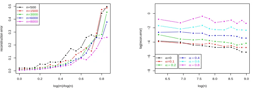
should be comparable to the one using the whole sample as long as α <0.5 . In Figure 1 (left panel) we plot the reconstruction errorkf¯ˆk−f
ρkHK versus the ratioα= log(m)/log(n)
for different sample sizes. We execute each simulationM = 30 times. The plot supports our theoretical finding. The right panel shows the reconstruction error versus the total number of samples using different partitions of the data. The black curve (α = 0) corresponds to the baseline error (m = 0, no partition of data). Error curves below a threshold α < 0.6 are roughly comparable, whereas curves above this threshold show a gap in performances.
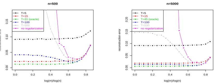
In another experiment we study the performances in case of (very) different regularization: Only partitioning the data (no regularization), underregularization (higher stopping index) and overregularization (lower stopping index). The outcome of this experiment amplifies the regularization effect of parallelizing. Figure 2 shows the main point: Overregulariza-tion is always hopeless, underregularizaOverregulariza-tion is better. In the extreme case of (almost) no regularization, there is a sharp minimum in the reconstruction error which is only slightly larger than the minimax optimal value for the oracle regularization parameter and which is achieved at an attractively large degree of parallelization. Qualitatively, this agrees very well with the intuitive notion that parallelizing serves as regularization.
We emphasize that numerical results seem to indicate that parallelization is possible to a slightly larger degree than indicated by our theoretical estimate. A similar result was reported in the paper Zhang et al. (2013), which also treats the low smoothness case.
4.2 High smoothness regime
We choose fρ(x) = 2π1 sin(2πx), which corresponds to just one non-vanishing Fourier
coef-ficient and by our criterion Corollary 11 has r=∞ . In view of our main Corollary 5 this requires a regularization method with higher qualification; we take the Gradient Descent
method (see Example 2).
The appearance of the term 2bmin{1, r}in our theoretical result 5 gives a predicted value
● ● ● ● ● ● ● ● ● ● ● ● ● ● ● ● ● ●
0.0 0.2 0.4 0.6 0.8
0.01 0.02 0.03 0.04 0.05 0.06 0.07 log(m)/log(n) reconstr uction error ● ● ● ● ● ● ● ● ● ● ● ● ● ● ● ● ● ● ● ● ● ● ● ● ● ● ● ● ● ● ● ● ● ● ● ● ● ● ● ● ● ● ● ● ● ● ● ● ● ● ● ● ● ● ● ● ● ● ● ● ● ● ● ● ● ● ● ● ● ● ● ● ● ● ● ● ● n=500 n=1500 n=3000 n=6000 n=9000 ● ● ● ● ● ● ● ● ● ● ● ●
6.5 7.0 7.5 8.0 8.5 9.0
−6 −5 −4 −3 −2 log(n) log(recon.error) ● ● ● ● ● ● ● ● ● ● ● ● ● ● ● ● ● ● ● ● ● ● ● ● ● ● ● ● ● ● ● ● ● ● ● ● ● ● ● ● ● ● ● ● ● ● ● ● ● ● ● ● ● ● ● ● ● ● ● ● ● ● ● α=0 α=0.2
α =0.4
●
● ●
α =0.6 α =0.7
α =0.8
Figure 1: The reconstruction error kf¯koracle
D −fρkHK in the low smoothness case. Left plot:
Re-construction error curves for various (but fixed) total sample sizes, as a function of the numbermof subsamples. Right plot: Reconstruction error curves for various subsample number scalingsm=nα, as a function of the sample size (on log-scale).
● ● ● ● ● ● ● ● ● ● ● ● ● ● ● ●
● ●
0.0 0.2 0.4 0.6 0.8
0.00 0.05 0.10 0.15 n=500 log(m)/log(n) reconstr uction error ● ● ● ● ● ● ● ● ● ● ● ● ● ● ● ● ● ● ● ● ● ● ● ● ● ● ● ● ● ● ● ● ● ● ● ● ● ● ● ● ● ● ● ● ● ● ● ● ● ● ● ● ● ● ● ● ● ● ● ● ● ● ● ● ● ● ● ● ● ● ● ● ● ● ● ● ● ● ● ● T=5 T=15 T=31 (oracle) T=100 T=500 no regularization ● ● ● ● ● ● ● ● ● ● ● ● ● ● ● ● ● ●
0.0 0.2 0.4 0.6 0.8
0.00 0.05 0.10 0.15 0.20 n=5000 log(m)/log(n) reconstr uction error ● ● ● ● ● ● ● ● ● ● ● ● ● ● ● ● ● ● ● ● ● ● ● ● ● ● ● ● ● ● ● ● ● ● ● ● ● ● ● ● ● ● ● ● ● ● ● ● ● ● ● ● ● ● ● ● ● ● ● ● ● ● ● ● ● ● ● ● ● ● ● ● ● ● ● ● ● ● ● ● ● ● ● ● ● ● T=5 T=15 T=45 (oracle) T=100 T=500 no regularization
Figure 2: The reconstruction errorkf¯λ
D−fρkHKin the low smoothness case. Left plot: Error curves
● ● ● ● ● ● ● ● ● ● ● ● ● ● ● ● ● ●
0.0 0.2 0.4 0.6 0.8
0.0 0.1 0.2 0.3 0.4 0.5 log(m)/log(n) reconstr uction error ● ● ● ● ● ● ● ● ● ● ● ● ● ● ● ● ● ● ● ● ● ● ● ● ● ● ● ● ● ● ● ● ● ● ● ● ● ● ● ● ● ● ● ● ● ● ● ● ● ● ● ● ● ● ● ● ● ● ● ● ● ● ● ● ● ● ● ● ● ● ● ● ● ● ● ● ● n=500 n=1500 n=3000 n=6000 n=8000 ● ● ● ● ● ● ● ● ● ● ●
6.5 7.0 7.5 8.0 8.5 9.0
−8 −6 −4 −2 0 log(n) log(recon.error) ● ● ● ● ● ● ● ● ● ● ● ● ● ● ● ● ● ● ● ● ● ● ● ● ● ● ● ● ● ● ● ● ● ● ● ● ● ● ● ● ● ● ● ● ● ● ● ● ● ● ● ● ● ● ● ● ● ● α=0 α=0.1
α =0.2
●
● ●
α =0.4 α =0.6
α =0.8
Figure 3: The reconstruction errorkf¯λoracle
D −fρkHK in the high smoothness case. Left plot:
Re-construction error curves for various (but fixed) sample sizes as a function of the number
mof subsamples. Right plot: Reconstruction error curves for various subsample number scalingsm=nα, as a function of the sample size (on log-scale).
no group of values of α performs roughly equivalently, meaning that we do not have any optimality guarantees.
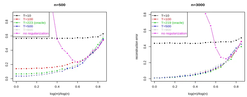
Plotting different values of regularization in Figure 4 we again identify overregularization as hopeless, while severe underregularization exhibits a sharp minimum in the reconstruction error. But its value at roughly 0.25 is much less attractive compared to the case of low smoothness where the error is an order of magnitude less.
5. Discussion
Minimax Optimality: We have shown that for a large class of spectral regularization methods the error of the distributed algorithmkT¯s( ¯fλn
D −fρ)kHK satisfies the same upper
bound as the error ¯
Ts(fλn
D −fρ)
H
K
for the single machine problem, if the regularization
parameter λn is chosen according to (16), provided the number of subsamples grows
suffi-ciently slowly with the sample size n. Since, the rates for the latter are minimax optimal (Blanchard and M¨ucke, 2017), our rates in Corollary 5 are minimax optimal also.
Comparison with other results: Zhang et al. (2013) derive minimax-optimal rates in three settings: finite rank kernels, sub-Gaussian decay of eigenvalues of the kernel and polynomial decay, provided m satisfies a certain upper bound, depending on the rate of decay of the eigenvalues under two crucial assumptions on the eigenfunctions of the integral operator associated to the kernel: For anyj∈N
● ● ● ● ● ● ● ● ● ● ● ● ● ● ● ● ● ●
0.0 0.2 0.4 0.6 0.8
0.0 0.2 0.4 0.6 0.8 n=500 log(m)/log(n) reconstr uction error ● ● ● ● ● ● ● ● ● ● ● ● ● ● ● ● ● ● ● ● ● ● ● ● ● ● ● ● ● ● ● ● ● ● ● ● ● ● ● ● ● ● ● ● ● ● ● ● ● ● ● ● ● ● ● ● ● ● ● ● ● ● ● ● ● ● ● ● ● ● ● ● ● ● ● ● ● ● ● ● ● ● ● ● ● ● ● ● ● T=10 T=100 T=223 (oracle) T=500 T=900 no regularization ● ● ● ● ● ● ● ● ● ● ● ● ● ● ● ● ● ●
0.0 0.2 0.4 0.6 0.8
0.0 0.2 0.4 0.6 0.8 n=3000 log(m)/log(n) reconstr uction error ● ● ● ● ● ● ● ● ● ● ● ● ● ● ● ● ● ● ● ● ● ● ● ● ● ● ● ● ● ● ● ● ● ● ● ● ● ● ● ● ● ● ● ● ● ● ● ● ● ● ● ● ● ● ● ● ● ● ● ● ● ● ● ● ● ● ● ● ● ● ● ● ● ● ● ● ● ● ● ● ● ● ● ● ● ● T=10 T=100 T=219 (oracle) T=500 T=900 no regularization
Figure 4: The reconstruction errorkf¯λ
D−fρkin the high smoothness case. Left plot: Error curves for
different stopping times forn= 500 samples, as a function of the number of subsamples. Right plot: Error curves for different stopping times forn= 5000 samples, as a function of the number of subsamples.
for some k ≥ 2 and ρ < ∞ or even stronger, it is assumed that the eigenfunctions are uniformly bounded, i.e.
sup
x∈X
|φj(x)| ≤ρ , (23)
or any j ∈N and some ρ <∞. We shall describe in more detail the case of polynomially decaying eigenvalues, which corresponds to our setting. Assuming eigenvalue decayµj .j−b
withb >1, the authors choose a regularization parameterλn=n−
b
b+1 and
m.
nb(k
−4)−k b+1
ρ4klogk(n)
1
k−2
.
leading to an error inL2-norm
E[kf¯Dλn−fρk 2 L2].n
−b+1b ,
being minimax optimal. Note that this choice of λn and the resulting rate correspond to
our case r= 0, i.e., no smoothness of fρ is assumed (just thatfρ belongs to the RKHS).
For k < 4 the bound becomes less meaningful (compared to the case where k ≥ 4) since
m → 0 as n → ∞ in this case (for any sort of eigenvalue decay). On the other hand, if
k and b might be taken arbitrarily large, corresponding to almost bounded eigenfunctions and arbitrarily large polynomial decay of eigenvalues, m might be chosen proportional to
bound given above, namely
m. n
b−1
b+1
ρ4logn ,
which for largebbehaves as above. Granted bounds on the eigenfunctions inL2kfor (very) largek, this is a strong result. While the decay rate of the eigenvalues can be determined by the smoothness ofK (see, e.g., Ferreira and Menegatto, 2009 and references therein), it is a widely open question which general properties of the kernel imply estimates as in (22) and (23) on the eigenfunctions.
Zhou (2002) even gives a counterexample and presents aC∞ Mercer kernel on [0,1] where the eigenfunctions of the corresponding integral operator arenotuniformly bounded. Thus, smoothness of the kernel is not a sufficient condition for (23) to hold.
Moreover, we point out that the upper bound (22) on the eigenfunctions (and thus the upper bound formin Zhang et al., 2013) depends on the unknown marginal distributionν. Only the strongest assumption, a bound in sup-norm (23), does not depend on ν. Concerning this point, our approach is ”agnostic”.
As already mentioned in the Introduction, these bounds on the eigenfunctions have been eliminated by Lin et al. (2017), for KRR, imposing polynomial decay of eigenvalues as above. This is very similar to our approach. As a general rule, our bounds on m and the bounds obtained by Lin et al. (2017) are worse than the bounds of Zhang et al. (2013) for eigenfunctions in (or close to )L∞, but in the complementary case where nothing is known on the eigenfunctionsmstill can be chosen as an increasing function ofn, namely m=nα. More precisely, choosing λn as in (16), Lin et al. (2017) derive as an upper bound
m.nα, α= 2br 2br+b+ 1 ,
withr being the smoothness parameter arising in the source condition. We recall here that due to our assumption q ≥r+s, the smoothness parameterr is restricted to the interval (0,12] for KRR (q = 1) andL2-risk (s= 12).
Our results (which hold for a general class of spectral regularization methods) are in some ways comparable to those of Lin et al. (2017). Specialized to KRR, our estimates for the exponent α in m =O(nα) coincide with the result of Lin et al. (2017). Furthermore, we emphasize that Zhang et al. (2013) and Lin et al. (2017) estimate the DL-error only for
s = 1/2 in our notation (corresponding to L2(ν)−norm), while our result holds for all values of s ∈ [0,1/2] which smoothly interpolates between L2(ν)-norm and RKHS-norm and, in addition, for all values of p ∈ [1,∞). Thus, our results also apply to the case of non-parametric inverse regression, where one is particularly interested in the reconstruction error, i.e. HK-norm (see, e.g., Blanchard and M¨ucke, 2017). Additionally, we precisely analyze the dependence of the noise varianceσ2 and the complexity radius Rin the source condition.
estimat-ing the approximation error and the sample error. The bias usestimat-ing a subsample should be of the same order as when using the whole sample, whereas the estimation error is higher on each subsample, but gets reduced by averaging by writing the variance as a sum of i.i.d. random variables (which allows to use Rosenthal’s inequality).
Finally, we want to mention the recent works of Lin and Zhou (2018) and Guo et al. (2017), which were worked out indepently from our work. Guo et al. (2017) also treat general spectral regularization methods (going beyond kernel ridge) and obtain essentially the same results, but with error bounds only inL2-norm, excluding inverse learning problems. Lin and Zhou (2018) investigate distributed learning on the example of gradient descent algorithms, which have infinite qualification and allow larger smoothness of the regression function. They are able to improve the upper bound for the number of local machines to
m. n
α
log5(n) + 1 , α <
br
2br+b+ 1,
which is larger in the case r >2. In the intermediate case 1< r <2, our bound in (20) is still better. An interesting feature is the fact that it is possible to allow more local machines by using additional unlabeled data. This indicates that finding the upper bound for the number of machines in the high smoothness regime is still an open problem.
Adaptivity: It is clear from the theoretical results that both the regularization parameter
λand the allowed cardinality of subsamplesmdepend on the parametersr andb, which in general are unknown. Thus, an adaptive approach to both parametersbandr for choosing
λ and m is of interest. To the best of our knowledge, there are yet no rigorous results on adaptivity in this more general sense. Progress in this field may well be crucial in fi-nally assessing the relative merits of the distributed learning approach as compared with alternative strategies to effectively deal with large data sets.
We sketch an alternative naive approach to adaptivity, based on hold-out in the direct case, where we consider each f ∈ HK also as a function in L2(X, ν). We split the data z ∈
(X × Y)n into a training and validation partz= (zt,zv) of cardinalitym
t, mv. We further
subdivide zt into mk subsamples, roughly of size mt/mk, where mk ≤ mt, k = 1,2, . . . is
some strictly decreasing sequence. For each k and each subsample zj, 1 ≤ j ≤ mk, we
define the estimators ˆfzλj as in (12) and their average
¯
fk,λzt :=
1
mk mk
X
j=1
ˆ
fzλj . (24)
Here,λvaries in some sufficiently fine lattice Λ. Then evaluation onzv gives the associated empiricalL2−error
Errλk(zv) := 1
mv mv
X
i=1
(yvi −f¯k,λzt(xvi))2 , zv = (yv,xv), yv = (yv1, . . . , ymv
v), (25)
leading us to define
ˆ
λk := argminλ∈ΛErrλk(zv), Err(k) := Err ˆ λk
k (z
Then, an appropriate stopping criterion fork might be to stop at
k∗:= min{k≥3 : ∆(k)≤δ inf
2≤j<k∆(j)}, ∆(j) :=|Err(j)−Err(j−1)|, (27)
for some δ <1 (which might require tuning). The corresponding regularization parameter is ˆλ= ˆλk∗, given by (26). At least intuitively, it is then reasonable to define a purely data
driven estimator as
b
fn:= ¯f ˆ λ
k∗,zt . (28)
Note that the training dataztenter the definition offbnvia the explicit formula (24) encoding our kernel based approach, while zv serves to determine (k∗,λˆ∗) via minimization of the empiricalL2-error and a criterion, which tells one to stop where Err(j) does not appreciably improve anymore. It is open if such a procedure achieves optimal rates, and we leave this for future research.
6. Proofs
For ease of reading we make use of the following conventions:
• for a (bounded) linear operator A,kAk denotes the operator norm;
• we are interested in a precise dependence of multiplicative constants on the parameters
σ, M, R, m, nand η. (To be clear about the role of the latter quantity: the proofs rely on high-probability statements on deviations, typically holding with high probability 1−η.)
• the dependence of multiplicative constants on various other parameters, including the kernel parameter κ, the interpolating parameter s ∈ [0,12], the parameters arising from the regularization method,b >1,β >0, r >0, etc. will (generally) be omitted and simply indicated by the symbolN.
• the dependence of the norm parameterp will also be indicated, but will not be given explicitly.
• the values ofCN and CN,p might change from line to line.
• the expression “for n sufficiently large” means that the statement holds forn ≥n0,
with n0 potentially depending on all model parameters (including σ, M and R), but
not on η.
6.1 Preliminaries
Proposition 12 (Guo et al., 2017, Proposition 1) Define
Bn(λ) :=
1 + 2
nλ +
r
N(λ)
nλ
!2
For any λ >0, η ∈(0,1], with probability at least 1−η one has
( ¯Tx+λ)−1( ¯T+λ)
≤8 log2(2η−1)Bn(λ). (30)
Corollary 13 Let η ∈(0,1). Forn∈N let λ˜n be implicitly defined as the unique solution
of N(˜λn) =nλ˜n. Then for any λ∈[max(˜λn, n−1),1], one has
Bn(λ)≤10.
In particular,
( ¯Tx+λ)−1( ¯T+λ)
≤80 log2(2η−1)
holds with probability at least 1−η.
We remark that the trace of ¯T is bounded by 1. This ensures that the interval [˜λn,1] is
non-empty.
Proof [of Corollary 13] Let ˜λn be defined via N(˜λn) = nλ˜n. Since N(λ)/λ is decreasing,
we have for any λ≥λ˜n
r
N(λ)
nλ ≤
s
N(˜λn) nλ˜n
= 1.
Inserting this bound as well as nλ≥1 into (29) and (30) leads to the conclusion.
Corollary 14 Assume the marginal distributionν ofX belongs toP<(b, β) withb >1and β >0. If λn is defined by (16) and if
mn≤nα, α <
2br
2br+b+ 1,
one has
B n
mn(λn)≤2,
provided nis sufficiently large.
Proof[of Corollary 14] We can for starters assume thatnis sufficiently large so thatλn<1,
i.e. λn =
σ2
R2n
2br+bb+1
from (16). Recall that ν ∈ P<(b, β) implies N(λ
n) ≤ CNλ
−1
b
n .
Looking at the terms entering inBn
m(λn), see (29), we have first, using the definition of λn
in (16):
N(λn) n mλn
≤CNmλ −b+1
b
n
n =CN m
n
nR2 σ2
2brb++1b+1
which (for fixed R, σ and other parameters entering in CN) is O(mnn−
2br
2br+r+1), and hence
o(1) provided
mn≤nα, α <
2br
2br+b+ 1 .
For the second term entering in Bn
m(λn), we have
1
n mλn
= m
n
nR2 σ2
2br+bb+1
,
which isO(mnn−
2br+1
2br+b+1) =o(1), provided
mn≤nα, α <
2br+ 1 2br+b+ 1 ,
which is implied by the previous stronger condition.
We shortly illustrate how Corollary 13 and Proposition 12 will be used. Let u ∈ [0,1], ˜
λn≤λas above andf ∈ HK. We have for any bounded operatorA
T¯uA
=
T¯u( ¯T+λ)−u( ¯T+λ)u( ¯Tx+λ)−u( ¯Tx+λ)uA
≤T¯u( ¯T+λ)−u
( ¯T+λ)u( ¯Tx+λ)−u
( ¯Tx+λ)uA
≤8 log2u(2η−1)Bn(λ)u( ¯Tx+λ)uA
, (31)
with probability at least 1−η, for any η ∈ (0,1); for the last inequality we have used that the first factor is less than 1, and for the second factor Proposition 12 in combination with the Cordes inequality (see Proposition 22 in the Appendix). In particular, for any max(˜λn, n−1)≤λ(with ˜λn as in Corollary 13)
T¯uA
≤80ulog2u(2η−1)
( ¯Tx+λ)uA
, (32)
with probability at least 1−η.
In the following, we constantly use (31). Furthermore, to bound terms involving residuals we will frequently use the following estimate: for v ≥0, u∈[0,2], and provided u+v≤q
(q being the qualification):
sup
t∈[0,1]
|rλ(t)tv(t+λ)u| ≤2
sup
t∈[0,1]
rλ(t)tv+u
+λu sup
t∈[0,1]
|rλ(t)tv|
≤CNλv+u, (33)
6.2 Approximation error bound
Recall that ν denotes the X-marginal of the sampling distribution ρ and P the set of all probability distributions on the input space X.
Lemma 15 Let ν ∈ P, v ∈ R and let x ∈ X n
m be an i.i.d. sample of size n/m, drawn
according to ν. Assume the regularization (gλ)λ has qualification q≥v+ 1 +s. Then with
probability at least 1−η:
T¯srλ( ¯Tx) ¯Txv( ¯T−Tx¯ )
≤CNlog4(4η−1)λs+v+1Bs+1n
m (λ)
m nλ +
r
mN(λ)
nλ
!
.
Proof [of Lemma 15] From (30),(31) and from Proposition 20 recalled in the Appendix, one has
T¯srλ( ¯Tx) ¯Txv( ¯T−Tx¯ )
≤CNlog2(s+1)(4η−1)Bs+1n
m (λ)
( ¯Tx+λ)srλ( ¯Tx) ¯Txv( ¯Tx+λ)
( ¯T +λ)−1( ¯T−Tx¯ )
≤CNlog4(4η−1)λs+v+1Bs+1n m
(λ) m
nλ +
r
mN(λ)
nλ
!
,
for anyλ∈(0,1], η∈(0,1], with probability at least 1−η. We also used thats≤ 12, and the estimate (33).
Lemma 16 Let ν ∈ P, v ∈ R and let x ∈ Xmn be an i.i.d. sample of size n/m drawn
according to ν. Assume the regularization (gλ)λ has qualification q ≥v+s. Then for any
λ∈(0,1], η∈(0,1], with probability at least 1−η
T¯srλ( ¯Tx) ¯Txv
≤CNlog2s(2η−1)Bsn
m(λ)λ
s+v ,
for some CN<∞.
Proof [of Lemma 16] Using (31), (33), sinceq ≥v+s, it holds
T¯srλ( ¯Tx) ¯Txv
≤CNlog2s(2η−1)Bsn
m(λ)
( ¯Tx+λ)srλ( ¯Tx) ¯Txv
≤CNlog2s(2η−1)Bsn
m(λ)λ
s+v ,
with probability at least 1−η.
Proposition 17 (Expectation of approximation error) Let fρ ∈ Ω(r, R), λ ∈ (0,1]
and let Bn
m(λ) be defined in (29). Assume the regularization has qualification q ≥ r+s.
1. If r≤1, then
h
Eρ⊗n
T¯s(fρ−f˜Dλ) p HK i1 p
≤CN,pR λs+rBs+rn
m (λ).
2. If r >1, then
h
Eρ⊗n
T¯s(fρ−f˜Dλ)
p HK
i1p
≤CN,pRλsBs+1n m
(λ) λr+λ m nλ +
r
mN(λ)
nλ
!!
.
In 1. and 2. the constantCN,p does not depend on (σ, M, R)∈R3+.
Proof [of Proposition 17] Sincefρ∈Ω(r, R),
h
Eρ⊗n
T¯s(fρ−f˜Dλ) p HK i1 p = h
Eρ⊗n
1 m m X j=1 ¯
Tsrλ( ¯Txj)fρ
p HK i1 p ≤ 1 m m X j=1 h
Eρ⊗n
T¯srλ( ¯Txj)fρ
p HK
i1p
≤ R m m X j=1 h
Eρ⊗n
T¯srλ( ¯Txj) ¯Tr
pi1p
. (34)
The first inequality is just the triangle inequality for the p-norm kfkp = E[kfkpHK]
1
p. We
bound the expectation for each separate subsample of size mn by first deriving a probabilistic estimate and then we integrate.
Consider first the case where r ≤1. Using (31), the Cordes inequality (Proposition 22 in the Appendix), and (33) one has for any j= 1, . . . , m,
T¯srλ( ¯Txj) ¯Tr
≤CNlog2(s+r)(4η−1)Bs+rn m
(λ)( ¯Txj+λ)
sr
λ( ¯Txj)( ¯Txj+λ)
r
≤CNlog3(4η−1)λs+rBs+rn m
(λ),
with probability at least 1−ηand where Bn
m(λ) is defined in (29). Recall that the
regular-ization has qualificationq≥r+s. By integration one has
h
Eρ⊗n
T¯srλ( ¯Txj) ¯Tr
pip1
≤CN,pλs+r Bs+rn m
(λ),
for someCN,p <∞, not depending on σ, M, R. Finally, from (34)
h
Eρ⊗n
T¯s(fρ−f˜Dλ)
p HK
i1p
≤CN,pR λs+r Bs+rn m
(λ).
In the case wherer ≥1, we writer=k+u, withk=brc andu=r−k <1. We shall use the decomposition
¯
Tk=
k−1
X
l=0
¯
We proceed by bounding (34) according to decomposition (35) . For anyj= 1, . . . , m, one has
h
Eρ⊗n
T¯srλ( ¯Txj) ¯Tk+u
pi1
p ≤ k−1 X l=0 h
Eρ⊗n
T¯srλ( ¯Txj) ¯Txl
j( ¯T −Tx¯ j) ¯T
k−(l+1)+u
pi1
p
+hEρ⊗n
T¯srλ( ¯Txj) ¯Txk
jT¯
u
pi1p
≤
k−1
X
l=0
h
Eρ⊗n
T¯srλ( ¯Txj) ¯Txl
j( ¯T −T¯xj)
pi1p
+ h
Eρ⊗n
T¯srλ( ¯Txj) ¯Txk
jT¯
u
pi1p
. (36)
Here we use that T¯k−(l+1)+u
is bounded by 1. By Lemma 16 and by (31), (33), with probability at least 1−η
¯
Tsrλ( ¯Txj) ¯T
k xjT¯
u
≤CNlog
2(s+u)(2η−1)Bs+u
n m
(λ)
( ¯Txj+λ)
sr
λ( ¯Txj) ¯T
k
xj( ¯Txj+λ)
u
≤CNlog2(s+u)(2η−1)Bs+un m
(λ)λs+r,
and thus integration yields
h
Eρ⊗n
T¯srλ( ¯Txj) ¯Txr
jT¯
u
pi1
p
≤CN,pBs+un
m (λ)λ
s+r. (37)
For estimating the first term in (36) we may use Lemma 15. For any l = 0, . . . , k−1, we have l+s+ 1 ≤ k+s ≤r+s ≤ q, hence for any j = 1, . . . , m with probability at least 1−η
¯
Tsrλ( ¯Txj) ¯T l xj( ¯T−
¯
Txj)
≤CNlog 4
(8η−1)λs+l+1Bs+1 n m (λ)
m nλ+
r
mN(λ)
nλ
!
.
Again by integration, since λl ≤1 for anyl= 0, . . . , k−1, one has
k−1 X
l=0 h
Eρ⊗n
T¯srλ( ¯Txj) ¯T l xj( ¯T−
¯
Txj)
pi1p
≤CN,pbrcλs+1Bs+1n m (λ)
m nλ+
r
mN(λ)
nλ
!
. (38)
Finally, combining (37) and (38) into (36), then (34), gives in the case where r >1
h
Eρ⊗n
T¯s(fρ−f˜Dλ)
p HK i1 p
≤CN,pλsBs+1n
m (λ) λ
r+λ m nλ+
r
mN(λ)
nλ
!!
.
Proof [of Theorem 3] Let λn be as defined by (16). According to Corollary 14, we have
B n
mn(λn) ≤ 2 provided α <
2br
2br+b+1, for n sufficiently large. We can also assume n
suffi-ciently large so thatλn<1, i.e., Rλr+sn =an (from (16), (17)). Under these conditions, we
immediately obtain from the first part of Proposition 17 in the case wherer≤1
h
Eρ⊗n
T¯s(fρ−f˜Dλn)
p HK
i1p
≤CN,pR λs+rn =CN,pan.
We turn to the case where r > 1. We apply the second part of Proposition 17. By Corollary 14 we have
h
Eρ⊗n
T¯s(fρ−f˜Dλn)
p HK
i1p
≤CN,pRλsnBs+1n mn
(λn)
λrn+λn
mn nλn
+ s
mnN(λn) nλn
≤CN,p Rλsn
λrn+λn
mn nλn
+√mn R σλ
r n
,
where we used that N(λn) ≤ CNλ
−1/b n and σ
r
λ−
1
b n
nλn =Rλ
r
n coming from the definition of λn, and λn<1. Furthermore,
mn nλn
=o √mnλrn
,
provided
mn≤nα, α <
2(br+ 1) 2br+b+ 1 .
Finally, for nsufficiently large, Rσ√mnλn≤1, provided that
α < 2b
2br+b+ 1 .
As a result, for any p≥1:
lim sup
n→∞
sup
ρ∈Mσ,M,R
h
Eρ⊗n
T¯s(fρ−f˜Dλn)
p HK
i1p
an
≤CN,p,
for someCN,p <∞, not depending on σ, M, R.
6.3 Sample error bound
Givenλ∈(0,1], we define the random variableξλ: (X ×R) n
m −→ HK by
ξλ(x,y) := ¯Tsgλ( ¯Tx)( ¯Txfρ−S¯x∗y).
Recall that according to Assumption (3), the conditional expectation w.r.t. ρ ofY givenX
satisfies
Eρ[Y|X=x] = ¯Sxfρ,
implying thatξλ has zero expectation (since ¯Tx= ¯Sx∗S¯x). Thus,
¯
Ts( ˜fDλ −f¯Dλ) = 1
m m
X
j=1
ξλ(xj,yj) (39)
is a sum of centered i.i.d. random variables.
Furthermore, we need the following result (Pinelis, 1994, Theorem 5.2) , which generalizes Rosenthal’s (1970) inequalities (originally only formulated for real valued random variables) to random variables with values in a Banach space. For Hilbert spaces this looks particularly nice.
Proposition 18 LetHbe a Hilbert space andξ1, . . . , ξmbe a finite sequence of independent,
mean zero H- valued random variables. If 2≤p <∞, then there exists a constantCp>0,
only depending on p, such that
E 1 m m X j=1 ξj p H !1 p
≤ Cp
m max
( m X
j=1
EkξjkpH
!1 p , m X j=1
Ekξjk2H
!1 2)
. (40)
We remark in passing that Dirksen (2011), Corollary 1.22, establishes the interesting result that in addition to the upper bound in (40) there is also a corresponding lower bound where the constantCp is replaced by another constant Cp0 >0, only depending onp.
Proposition 19 (Expectation of sample error) Let ρ be a source distribution
belong-ing toMσ,M,R, s∈[0,12] and let λ∈(0,1]. Define Bn
m(λ) as in (29). Assume the
regular-ization has qualification q ≥r+s. For any p≥1 one has:
h
Eρ⊗n
T¯s( ˜fDλ −f¯Dλ)
p HK
i1p
≤CN,pm−
1 2Bn
m(λ)
1
2+sλs mM
nλ +σ
r
mN(λ)
nλ
!
,
where Cp does not depend on(σ, M, R)∈R3+.
Proof [of Proposition 19] Letλ∈(0,1] andp≥2. From Proposition 18
Eρ⊗n
¯
Tsf˜Dλ −f¯Dλ
p HK 1p = "
Eρ⊗n
1 m m X j=1
ξλ(xj,yj)
p HK
#1p
≤ Cp
m max ( m X j=1 h
Eρ⊗nkξλ(xj,yj)kpH K i 1 p , m X j=1 h
Again, the estimates in expectation will follow from integrating a bound holding with high probability. By (31), one has for any j= 1, . . . , m,
kξλ(xj,yj)kHK =kT¯
sg
λ( ¯Txj)( ¯Txjfρ−S¯
∗
xjyj)kHK
≤8 log2s(4η−1)Bn
m(λ)
sk( ¯Tx
j +λ)
sg
λ( ¯Txj)( ¯Txjfρ−S¯
∗
xjyj)kHK , (42)
holding with probability at least 1− η2, where Bn
m(λ) is defined in (29). We proceed by
splitting:
( ¯Txj+λ)
sg
λ( ¯Txj)( ¯Txjfρ−S¯
?
xjyj) =H
(1) xj ·H
(2) xj ·h
λ zj ,
with
Hx(1)j :=||( ¯Txj+λ)
sg
λ( ¯Txj)( ¯Txj +λ)
1 2||,
Hx(2)j :=||( ¯Txj+λ)
−1
2( ¯T +λ) 1 2||,
hλzj :=||( ¯T+λ)−12( ¯Tx
jfρ−S¯
?
xjyj)||HK .
The first term is estimated using (9),(10) and gives for s∈[0,12]
Hx(1)j ≤ sup
t∈[0,1]
gλ(t)(t+λ)s+
1 2
≤2
sup
t∈[0,1]
gλ(t)ts+
1 2 +λs+
1 2 sup
t∈[0,1] gλ(t)
≤2
sup
t∈[0,1] gλ(t)
12−s sup
t∈[0,1] gλ(t)t
s+12
+λs+12 sup
t∈[0,1] gλ(t)
≤CNλs−12 . (43)
The second term is now bounded using (31) once more. One has with probability at least 1−η4
Hx(2)j ≤8 log(8η
−1
)Bn
m(λ)
1
2 . (44)
Finally, hλzj is estimated using Proposition 21:
hλzj ≤2 log(8η−1) mM
n√λ+σ
r
mN(λ)
n
!
, (45)
holding with probability at least 1−η4. Thus, combining (43), (44) and (45) with (42) gives for any j= 1, . . . , m,
kξλ(xj,yj)kHK ≤CNlog
2(s+1)(8η−1
)Bn
m(λ)
1
2+sλs mM
nλ +σ
r
mN(λ)
nλ
!
,
with probability at least 1−η. Integration gives for any p≥2:
m
X
j=1
h
Eρ⊗n
ξλ(xj,yj)
p HK
i
with
A:=An
m(λ) :=B
n
m(λ)
1
2+sλs mM
nλ +σ
r
mN(λ)
nλ
!
.
Combining this with (41) implies, sincep≥2:
h
Eρ⊗n
T¯s( ˜fDλ −f¯Dλ)
p HK
i1p
≤ CN,p
m max
(mAp)1p, mA2
1 2
= CN,p
m Amax
m1p, m12
= C√N,p
m A,
whereCN,p does not depend on (σ, M, R)∈R3+. The result for the case 1≤p≤2
immedi-ately follows from H¨older’s inequality.
Proof [of Theorem 4] Let λn be as defined by (16); as earlier we assume n is big enough
so thatλn<1. According to Corollary 14, we have Bmn(λn)≤2 provided α < 2br+b+12br and nis sufficiently large. Under this condition we immediately obtain from Proposition 19:
h
Eρ⊗n
T¯s( ˜fDλn−f¯Dλn)
p HK
ip1
≤ C√N,p
m λ s n mM nλn +σ s
mN(λn) nλn
≤CN,pλsn
√ mM nλn +σ s λ− 1 b n nλn ,
where we used again that N(λn)≤CNλ
−1/b n ; now
√
mnM nλn
=o
σ s
λ−1/bn nλn
,
provided
mn≤nα, α <
2(br+ 1) 2br+b+ 1 .
Recalling that σ
q
λ−n1/b
nλn =Rλ
r
n=λ−sn an, we arrive at
h
Eρ⊗n
T¯s( ˜fDλn−f¯Dλn)
p HK
i1p
≤CN,pan.
As a result, for any p≥1:
lim sup
n→∞
sup
ρ∈Mσ,M,R
h
Eρ⊗n
T¯s( ˜fDλn−f¯Dλn)
p HK
i1p
an
≤CN,p,
for someCN,p, not depending on the model parameters (σ, M, R)∈R3+, thus leading to the
Appendix A
Proposition 20 (see e.g. Blanchard and M¨ucke, 2017, Proposition 5.3) For anyn∈
N, λ∈(0,1] andη ∈(0,1), one has with probability at least 1−η:
( ¯T+λ)−1( ¯T−T¯x)
HS ≤2 log(2η
−1) 2 nλ +
r
N(λ)
nλ
!
,
where k.kHS denotes the Hilbert-Schmidt norm. (Since the operator norm is bounded by the
Hilbert-Schmidt norm, the above statement also holds for the operator norm.)
Proposition 21 (see e.g. Blanchard and M¨ucke, 2017, Proposition 5.2) For n ∈
N, λ∈(0,1] andη ∈(0,1], it holds with probability at least 1−η:
( ¯T +λ)−12 T¯xfρ−S¯?
xy H
K ≤ 2 log(2η
−1) M n√λ+
r
σ2N(λ) n
!
.
Proposition 22 (Cordes Inequality, see e.g. Bhatia, 1997, Theorem IX.2.1-2) Let
A, B be to self-adjoint, positive operators on a Hilbert space. Then for anys∈[0,1]:
kAsBsk ≤ kABks . (46)
References
F. Bauer, S. Pereverzev, and L. Rosasco. On regularization algorithms in learning theory.
J. Complexity, 23(1):52–72, 2007.
R. Bhatia. Matrix Analysis. Springer, 1997.
G. Blanchard and N. M¨ucke. Optimal rates for regularization of statistical inverse learning problems. Foundations of Computational Mathematics, 2017.
X. Chang, S.-B. Lin, and Y. Wang. Divide and conquer local average regression. Electron.
J. Statist., 11(1):1326–1350, 2017. doi: 10.1214/17-EJS1265. URL https://doi.org/
10.1214/17-EJS1265.
G. Cheng and Z. Shang. Computational limits of divide-and-conquer method. Technical report, arXiv:1512.09226, 2016.
E. De Vito and A. Caponnetto. Optimal rates for regularized least-squares algorithm.
Foundations of Computational Mathematics, 7(3):331–368, 2006.
S. Dirksen. Noncommutative and vector-valued Rosenthal inequalities. PhD thesis, Delft Univ. Technology, 2011.
H. Engl, M. Hanke, and A. Neubauer.Regularization of Inverse Problems. Kluwer Academic Publishers, 2000.
J. C. Ferreira and V. A. Menegatto. Eigenvalues of integral operators defined by smooth positive definite kernels. Integral Equations and Operator Theory, 64(1):61–81, May 2009. ISSN 1420-8989.
L. L. Gerfo, L. Rosasco, F. Odone, E. De Vito, and A. Verri. Spectral algorithms for supervised learning. Neural Computation, 20(7):1873–1897, 2008.
Q. Guo, B.-W. Chen, S. Rho, W. Ji, F. Jiang, X. Ji, and S.-Y. Kung. Efficient divide-and-conquer classification based on parallel feature-space decomposition for distributed systems. IEEE Systems Journal, 2015.
Z.-C. Guo, S.-B. Lin, and D.-X. Zhou. Learning theory of distributed spectral algorithms.
Inverse Problems, 33(7):074009, 2017.
C. J. Hsieh, S. Si, and I. Dhillon. A divide-and-conquer solver for kernel support vector machine. Proceedings of the 31. International Conference on Machine Learning, 32(1): 575–583, 2014.
R. Li, D. K. J. Lin, and B. Li. Statistical inference in massive data sets. Applied Stochastic
Models in Business and Industry, 29 (5):399–409, 2013.
S. Lin, X. Guo, and D.-X. Zhou. Distributed learning with regularized least squares.Journal
of Machine Learning Research, 18:1–31, 2017.
S.-B. Lin and D.-X. Zhou. Distributed kernel-based gradient descent algorithms.
Construc-tive Approximation, 47(2):249–276, 2018.
L. Mackey, A. Talwalkar, and M. I. Jordan. Divide-and-conquer matrix factorization.
Ad-vances in Neural Information Processing Systems 24 (NIPS 2011), 2011.
I. Pinelis. Optimum bounds for the distributions of martingales in Banach spaces. The
Annals of Probability, 22(4):1679–1706, 1994.
H. P. Rosenthal. On the subspaces of Lp (p > 2) spanned by sequences of independent random variables. Israel J. Math., 8:273–303, 1970.
C. Xu, Y. Zhang, R. Li, and X. Wu. On the feasibility of distributed kernel regression for big data. IEEE Transactions on Knowledge and Data Engineering, 28:3041–3052, 2016.
Y. Zhang, J. Duchi, and M. Wainwright. Divide and conquer kernel ridge regression. JMLR:
Workshop and Conference Proceedings, 30:1–26, 2013.