206
This work is licensed under Creative Commons Attribution 4.0 International License.
Numerical Simulation of Helically Coiled Closed Loop Pulsating Heat Pipe
Bhagwat Adhikari1 and Dr. Sanjeev Maharjan2
1Student, Department of Mechanical Engineering, IOE-Pulchowk Campus, NEPAL 2Professor, Department of Mechanical Engineering, IOE-Pulchowk Campus, NEPAL
1
Corresponding Author: [email protected]
ABSTRACT
This paper addresses the numerical simulation of helically coiled closed loop pulsating heat pipe which is carried in ANSYS Fluent. The values of thermal resistance for constant heat fluxes vs. transient heat fluxes are analyzed. Phase change visualization after the end of simulation is carried out to observe the phenomenon in liquid at its saturation temperature and pressure. Finally, helical heat pipes are found to have thermal resistance less by 2.7K/W, 0.56 K/W, and 0.227 K/W for 8W, 40W and 80W heat inputs than circular pipes. Helical heat pipes are found more efficient than circular heat pipes.
Keywords— Helical, pulsating heat pipe, simulation, thermal resistance
Table 1: List of Abbreviations Abbreviations
Q Heat
Te Evaporator temperature
Tc Condenser temperature
R Thermal resistance
p pressure
Nu Nusselt number
Pr Prandtl number
Re Reynold's Number
S Source Term
Coeff. coefficient to be tuned
v vapor
V Velocity
T Temperature
hs condensation heat transfer coefficient
x vapor quality
Cp,w effective heat capacity of wall
kw thermal conductivity of wall
I.
INTRODUCTION
An efficient heat transfer technology the subject of research globally. The amount of fossil fuels from the earth
crust has been declining and is towards extinction. In addition to this, the global warming caused by the use of fossil fuels has compelled the researchers to find an alternative solution which can address the problem. In the area of automobile, an alternative to combustion engine can be high voltage battery which could deliver the same amount of power and torque. Similarly, the electric generation via use of coal may be possibly replaced by the use of solar energy to produce electricity. The storage and effective transfer of thermal energy system is thought to be crucial in near future.
Heat pipes are recognized as one of the most efficient passive heat transfer technologies available. A heat pipe is a structure with very high thermal conductivity that enables the transportation of heat whilst maintaining almost uniform temperature along its heated and cooled sections. In general, heat pipes are passive thermal transfer devices able to transport large amounts of heat over relatively long distances, with no moving parts, using phase-change processes and vapor diffusion. The main structure of a heat pipe consists of an evacuated tube partially filled with a working fluid that exists in both liquid and vapor phases.
The application of the heat pipes is widely known. The high voltage battery in hybrid-electric, electric vehicles is said to have maximum efficiency at the temperature of 35 0
C. In order to maintain this temperature, the heat generated from the battery has to be dissipated to the surrounding which needs an efficient heat transfer medium. Heat pipes are being experimented in this field to solve the issue. Also, in order to transfer the solar thermal energy the people working in the area of cryogenics fluid is trying to build the heat pipe system. Industries are challenging the heat transfer community to provide solutions to enable systems that can run reliably at extremely cold temperatures. Theoretically, a heat pipe can operate at any given temperature, as long as the operation temperature is between the triple and the critical points of the working fluid utilized.
207
This work is licensed under Creative Commons Attribution 4.0 International License.
creating new areas of implementation for heat pipe basedsystems. In addition, with advances in automation and development in material sciences, new heat pipe materials has to be investigated to deal with challenging areas that have so far been out of reach for conventional solutions, particularly in dealing with high temperature and strongly contaminated flows. The addition of heat pipes in a range of temperature scales and applications are a clear indication of the potential for such a technology, but there are significant modeling issues which are hindering the performance. The lack of advancements within commercial models will result in the increase of bespoke codes created in open source software. The use of nano fluids can be considered important for the future of heat pipes, but the validity of such claims is questionable with the lack of validation. Extensive research still needs to be conducted on Newtonian fluids before progression onto other fluids.
The search for cost effective, reliable and efficient thermal management system is constantly growing. Likewise, research works trying to establish PHP as a novel device to manage the heat flux problem in wider range of application has attracted many scientists. PHP is seen as potential heat controlling devices in the field of microprocessors, solar panel, fuel cells, space exploration and many more. Once the operational features of PHP are fully established, PHP is certain to get a commercial platform
Theoretical and Numerical Modeling of PHP Assumptions
In order to model heat transfer and flow characteristics in the theoretical model, the following assumptions are made:
The vapor quality in the evaporator and condenser is in linear variation along the flow direction, and no variation in adiabatic section.
The liquid is incompressible and the vapor is assumed to behave as an ideal gas, both in the saturated state for ammonia working fluid during experiment temperature area.
The heat losses causing by the convection and radiation heat transfer between the ambient to the tube wall of whole PHP are neglected
Governing Equations Lee Model
The Lee model is used with the mixture and VOF multiphase models. In the Lee model, the liquid-vapor mass transfer (evaporation and condensation) is governed by the vapor transport equation:
𝜕(𝛼𝑣𝜌𝑣)
𝜕𝑥 + 𝛻 ∙ 𝛼𝑣𝜌𝑣𝑉 𝑣 = 𝑚 𝑙𝑣− 𝑚 𝑣𝑙
If Tl>Tsat (evaporation):
𝑚 𝑙𝑣 = 𝑐𝑜𝑒𝑓𝑓 ∗ 𝛼𝑙 𝜌𝑙(𝑇𝑙− 𝑇𝑠𝑎𝑡)/𝑇𝑠𝑎𝑡
If Tl<Tsat (condensation):
𝑚 𝑣𝑙 = 𝑐𝑜𝑒𝑓𝑓 ∗ 𝛼𝑣 𝜌𝑣(𝑇𝑠𝑎𝑡 − 𝑇𝑣)/𝑇𝑠𝑎𝑡
Where,
𝛼𝑣 = vapor volume fraction
𝛼𝑙 = liquid volume fraction
𝜌𝑣 = vapor density
𝑉 𝑣 = vapor phase velocity
𝑚 𝑙𝑣,𝑚 𝑣𝑙 = the rates of mass transfer due to evaporation and
condensation
Coeff. = coefficients to be tuned which is termed as evaporation and condensation frequency
Volume Fraction Equation
The tracking of the interface(s) between the phases is accomplished by the solution of a continuity equation for the volume fraction of one (or more) of the phases. For the „w‟ phase, this equation has the following form:
1 𝜌
𝜕
𝜕𝑡 𝛼𝑙𝜌𝑙 + 𝛻 ∙ 𝛼𝑙𝜌𝑙𝑣 𝑙 = 𝑆𝛼𝑙+ 𝑚 𝑣𝑙− 𝑚 𝑙𝑣
𝑛
𝑣=1
where, 𝑚 𝑣𝑙is the mass transfer from phase „v‟ to
phase „l‟ and 𝑚 𝑙𝑣 is the mass transfer from phase „l‟ to
phase „v‟. By default „S‟, the source term on the right-hand side of above equation is zero
The volume fraction equation will not be solved for the primary phase; the primary-phase volume fraction will be computed based on the following constraint:
𝛼𝑙 = 1
𝑛
𝑙=1
Condensation
The value of condensation heat transfer is determined by the two factors, which are condensation heat transfer coefficient hs and vapor quality x. While hs has a direct relationship with the velocity of fluid flow in the condenser, and the quality x relates the distribution of liquid and vapor phase. Obviously, these two items are all varied as the flow patterns change.
One of the most widely used has been the shah‟s correlation, covering three flow regimes, such as the If the flow pattern is in „„Slug Flow”, the vapor will flow through the condenser section slowly, and the mechanism of condensation is used following heat transfer equation,
𝑠= 1.32 ∙ 𝑅𝑒𝐿𝑆−1/3
𝜌𝑙 𝜌𝑒− 𝜌𝑔 ∙ 𝑔 ∙ 𝑠𝑖𝑛𝛽 ∙ 𝑘𝑙3
𝜇𝑙2
1/3
where, ReLS is Reynolds number assuming liquid phase flowing in tube alone.
Above figure shows a schematic of annular flow pattern features at high input power in PHP tubes.
208
This work is licensed under Creative Commons Attribution 4.0 International License.
𝑁𝑢 = 0.023𝑅𝑒𝑙𝑠0.8𝑃𝑟𝑙0.4[ 1 − 𝑥 0.8
+ 3.8𝑥0.76 1 − 𝑥 0.04/𝑃𝑟0.38]
Where, the „Pr‟ is the reduced pressure of vapor in the entrance of condenser.
Characteristics of Helical Coil
Inner diameter of pipe is 2r and the coil diameter is 2Rc (measured between the centers of pipes) .Dean number is used to characterize the flow in helical pipe as same to Reynolds number for flowing pipes. Dean number (De):
𝐷𝑒 = 𝑅𝑒 𝑟
𝑅𝑐
where Re is the Reynolds number.
Mathematical Model
Figure 1: Schematic diagram of helical oscillating heat pipe
Same as circular pulsating heat pipe HOHP consists of three parts: the evaporator section (Le), the adiabatic section (La) and the condenser section (Lc), with the coil radius ra, the pitch ps, the radius a (defined by the increase in elevation per revolution of coils hg= 2ps, the curvature ratio and the torsion , which can be calculated using
𝑘 = 𝑟𝑎
2
𝑟𝑎2+ 𝑝𝑠2
𝜏 = 𝑝𝑠
2
𝑟𝑎2+ 𝑝𝑠2
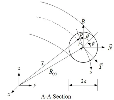
Figure shows an orthogonal helical coordinate system. The basic governing equations for helical tubes can be represented in an orthogonal helical coordinate system, as suggested by Germano (1982). An orthogonal helical coordinate system can be introduced with respect to a master Cartesian coordinate system (x, y, z), by using the helical coordinates s for the axial direction, r for the radial direction and for the circumferential direction.
Figure 2: Cylindrical coordinate system for heat pipe
The vector in the orthogonal coordinate system of a HOHP isR(s) , as calculated by
𝑅(𝑠)
= 𝑎𝑐𝑜𝑠 𝑠 𝑖 + 𝑎 𝑠𝑖𝑛 𝑠 𝑗 + 𝑏 𝑠 𝑘
The position of any given point p inside the helical pipe can be described by the vector X, which can be calculated as
𝑋 = 𝑅 − 𝑟𝑠𝑖𝑛 𝜃 − 𝜏𝑠 𝑁𝑠 + 𝑟 𝑐𝑜𝑠 𝜃 − 𝜏𝑠 𝐵𝑠 𝑠
Where T , N , B are the tangential, normal and bi-normal directions to the generic curve of the pipe axis R(s) at the point of consideration, respectively. The metric of the orthogonal helical coordinate system is given by:
𝑑𝑥 ∙
𝑑𝑥 = (1 + 𝑘𝑟𝑠𝑖𝑛 𝜃 − 𝜏𝑠 )2𝑑𝑠2+ 𝑑𝑟2+ 𝑟2𝑑𝜃2
where dr, ds and d are the infinitesimal increments in the radial, axial and circumferential directions, respectively. With this metric, one obtains the scale factor hs as given by
𝑠= 1 + 𝑘𝑟𝑠𝑖𝑛 𝜃 − 𝜏𝑠
Governing Equations
Governing equations for the calculated of the HOHP are the governing equation at the pipe wall and the vapor core. In addition, there is the governing equation for calculation of the heat transfer. All of which can be describe as in the following.
Heat Conduction of the Pipe Wall
Under normal operation, the heat applied to the evaporator section by an external source is conducted through the pipe wall. The three-dimensional transient condition heat conduction equation that describes the temperature in the heat pipe wall from conservation of energy is
𝜌𝑤𝐶𝑝,𝑤
𝛿𝑇𝑤
𝛿𝑡 =
𝑘𝑤
𝑟 𝛿
𝛿𝑟 𝑟
𝛿𝑇𝑤
𝛿𝑟 +
𝑘𝑤
𝑟
𝛿2𝑇
𝑤
𝛿𝜃2 + 𝑘𝑤
𝛿2𝑇
𝑤
𝛿𝑧2
209
This work is licensed under Creative Commons Attribution 4.0 International License.
where Cp,w is the effective heat capacity of the pipe wall,and kw is the effective thermal conductivity of the pipe wall.
Vapor Core
The continuity, the momentum and the energy equations used in the calculation at the vapor core of the HOHP are given
Continuity Equation:
𝜕𝑟𝑤
𝜕𝑠 = 0
Momentum Equation
𝜕𝑤
𝜕𝑡 +
1 𝑠
𝜕𝑤
𝜕𝑠 +
𝑘𝑠𝑖𝑛(𝜃 − 𝜏𝑠) 𝑠
𝑤 +𝑘𝑐𝑜𝑠(𝜃 − 𝜏𝑠)
𝑠
𝑤
= −1
𝑠
𝜕𝑝
𝜕𝑠+
1 𝑅𝑒
1 𝑠
𝜕 𝜕𝑠
1 𝑟𝑠
𝜕𝑟𝑤
𝜕𝑠
Energy Equation
𝜕𝑇
𝜕𝑡+
𝑤 𝑠
𝜕𝑇
𝜕𝑠=
1 𝑅𝑒𝑃𝑟
1 𝑠𝑟
𝜕 𝜕𝑠
𝑟 𝑠
𝜕𝑇
𝜕𝑠
II.
METHODOLOGY
Geometry
. Since the simulation is expensive in terms of computation, the number of turns is taken as four. The geometry for the figure shown above is taken from the experimental work performed by Pachghare (2014) in order to valid and verify the results before proceeding with the helical structure because much researches has not been done in the area of helical oscillating heat pipe.
Figure 3: Schematic of model for simulation
Table 2: Design parameters for helical heat pipe
Length of Evaporator 100mm
Length of Condenser 100mm
Number of turns 2.5
Diameter of coil 80mm
Diameter of pipe 2mm
Pitch 40mm
Physics Setup
On the basis of the experiment performed by Pachghare, et al. (2014) following simulating criteria is selected.
Table 3: Physics setup
SN Domain/Boundary/Physics Type
1 Fluid Model Volume of Fluid
(Lee Model) 2 Time step for Transient
Analysis
0.0003
3 Materials: Water Liquid & Vapor
4 Evaporation and
Condensation Model
For phase change
5 Saturation Temp & Pressure 308K & 4kPa
6 Convergence Criteria 10^-3
7 Solver: Solution Method SIMPLE
8 Wall material Copper
Boundary Conditions
First simulation is tested with 80W heat input on the evaporator in which the heat fluxes are provided directly to the walls of evaporator. This is the Neumann boundary condition because it involves the value obtained from the derivate of thermal energy per unit area with respect to time. In some of the experiments performed by researchers (Yeboaha et. al (2018)), the walls of evaporator is heated by a hollow cylindrical pipe in which a hot liquid flows.
The temperature in condenser should be less than the saturation temperature; otherwise, the phase change won‟t occur there. Thus condenser of the heat pipe is maintained at 302 degree Kelvin.
Zero heat flux is assigned to the adiabatic section because Fluent recognizes the insulation area with this value.
Copper, whose thickness is taken as 0.5mm, is selected as wall material as it is preferred as solid material for heat pipes due to its high thermal conductivity.
Solution Controls
The Courant number is adaptive and was not fixed for the simulation to run. The under relaxation factors for momentum and pressure were take as 0.3 each because solution converged soon as this value was decreased from the default value of 0.7.
Initial Conditions
210
This work is licensed under Creative Commons Attribution 4.0 International License.
III.
RESULTS AND DISCUSSIONS
Tuning of coefficients in Lee Model
The coefficients in the Lee Model has to be tuned which is the case of hit and trial to verify the case as similar to heat pipe. Therefore, before proceeding to the simulation in heat pipe, a simple case was studied in a cube which has the following case.
In a closed cubical cylinder 25% of the volume is occupied by saturated water of mass (ml) 1.4kg and rest by saturated steam at 200 deg Celsius. When “Q” amount of heat to be supplied to water the water should evaporate completely within 12.88sec.
Calculation of Q and Tuning of Lee Coeffients
Using iterative method for Lee coefficient we obtain [Source of Lee] value of 0.0008. The Lee coefficient signifies that the mass of water of 1.4 kg at saturation temperature of 200C completely converts to vapor phase with addition of Q = 3.9 MW in 14.9 sec.
Figure 4: Steam volume fraction at t=0
Figure 5: Steam volume fraction at t=14.89
Figure 6: Steam Volume fraction at t=14.9
Different to the circular structure, the thermal resistance curve in helical first increases to the certain amount of heat input and decreases. It is not the area of interest beyond the value greater than 90W because heat pipe is not suitable to transport this amount of heat from evaporator to condenser that can result in dry out condition.
Effect of Transient Evaporator Heat Flux in Helical Pipe
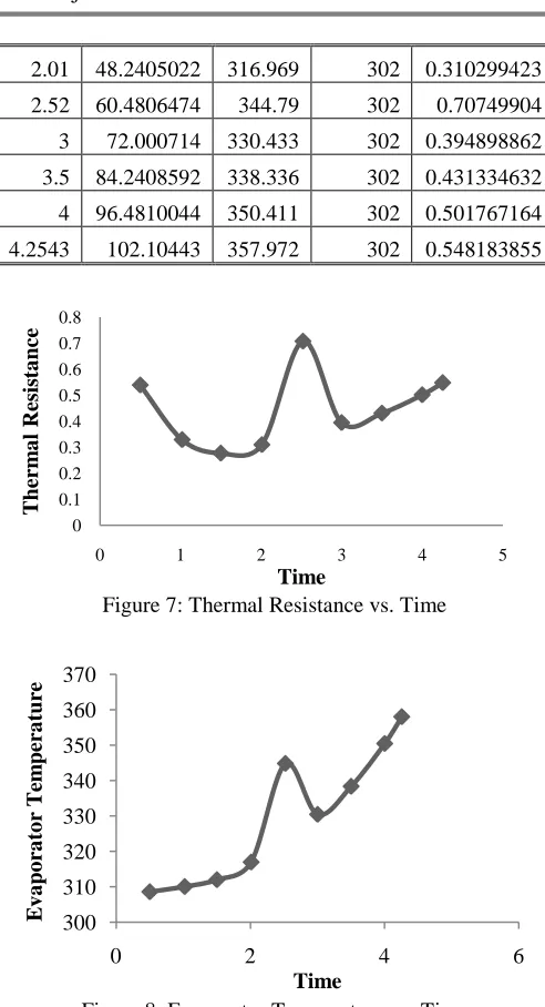
In helical OHP, at a certain point in evaporator the value of different parameters such as thermal resistance, heat flux, steam volume fraction, difference in thermal potentials are observed. At t= 0.5, thermal resistance is found to be 0.54. As the rate of heat input from the evaporator increase, thermal resistance decreases until a constant value of 0.3 K/W is reached. At this stage the heat flux in the evaporator is 20252 W/m2. After increasing the heat flux to a amount of 25390 W/m2, the thermal resistance value increases drastically to 0.7 K/W. The increase in thermal resistance in that spot is due to the formation of vapor near to that region which pushes the liquid slug. The thermal energy in vapor phase is more than in liquid phase which heats up the wall of the evaporator. Hence, at this time, the circulation of the fluid commences resulting in the flow of liquid and vapor periodically in a particular region. The time of start of the circulation was found to be 2.52s from the simulation result. As the time elapses, the thermal resistance value at the particular region in evaporator shows the same behavior as in previous time period.
Table 4: Different thermal parameters value obtained from simulation
t(s) Qin(Watt) Te(K) Tc(K) R
0.5 12.2401452 308.6 302 0.53920929
1.02 24.4802904 310.067 302 0.329530405
211
This work is licensed under Creative Commons Attribution 4.0 International License.
2.01 48.2405022 316.969 302 0.3102994232.52 60.4806474 344.79 302 0.70749904
3 72.000714 330.433 302 0.394898862
3.5 84.2408592 338.336 302 0.431334632
4 96.4810044 350.411 302 0.501767164
4.2543 102.10443 357.972 302 0.548183855
Figure 7: Thermal Resistance vs. Time
Figure 8: Evaporator Temperature vs. Time
Figure 9: Thermal Resistance vs. Heat Input
The temperature of evaporator at a particular region increases linearly at first because the wall heats up taking the sensible heat flux at first and increases drastically due to the energy of the vapor phase formed by taking evaporative heat.
Start Up Performance of Helical Heat Pipe
After heat is supplied to the evaporator, the vapor generation starts as the saturation temperature is reached. Due to the uniform heat flux in the evaporator, the vapor generation starts everywhere downside and upside of the curve. Due to gravity, the vapor bubbles from the upper part descend to the lower region where it coalesce with the bubbles formed in the lower region resulting in the formation of liquid and vapor slug. As this process continues, the vapor pressure in the evaporator region rises till it‟s sufficient to drive the liquid and slug of vapor from evaporator to the condenser region. The amount of time taken for one single liquid slug to move from the evaporator to condenser region and back to evaporator is called the start up time.
Annular Flow
Annular flows in pipes are the flows that mostly occur in bends. The liquid and vapor slugs change the shape of the flow from circular to the angular due to the centrifugal force and secondary flows.
Slug Flow
Slugs of liquid and vapor are formed when the large amount of vapors combine which are formed at different intervals of time. When sufficient amount of heat is supplied to the evaporator, the change in the thermal energy to the vapor pressure energy starts the circulation of these slugs against the buoyant and surface tension forces.
Bubble Flow
The formation of bubble is seen at the initial stage of heating of the heat pipe. Some amount of bubbles strike the walls losing its kinetic energy; some starts growing in diameter due to coalesce of the vapors.
Stratified Flow
The flow in which the bubbles and slugs in conjunction is known as stratified flow.
The enhancement in heat transfer in helical pipe is due to the complex flow pattern existing inside the pipe. The helix angle and the pitch of the coil results in the torsion of the fluid and the curvature of the coil determines the centrifugal force. The centrifugal force develops a secondary flow inside the helical tube. The curvature effect makes the fluid in the outer side of the pipe to move faster than that present inside, which gives a difference in velocity setting up a secondary flow which changes correspondingly with the Dean number of the flow.
0 0.1 0.2 0.3 0.4 0.5 0.6 0.7 0.8
0 1 2 3 4 5
T
herm
a
l
Resis
ta
nce
Time
300 310 320 330 340 350 360 370
0 2 4 6
E
v
a
po
ra
to
r
T
em
pera
ture
Time
0 0.1 0.2 0.3 0.4 0.5 0.6 0.7 0.8
0 20 40 60 80 100 120
T
h
er
m
a
l
R
esi
st
a
n
ce
212
This work is licensed under Creative Commons Attribution 4.0 International License.
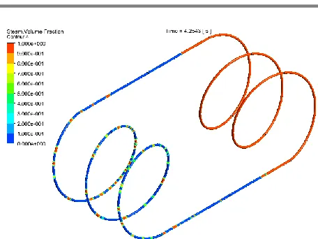
Figure 10: Steam volume fraction at t=4.25 for transientheat input with different bubbles and slugs shown
IV.
CONCLUSION
From the simulation of the cubical cylinder, the evaporation frequency to carry out this simulation was found to be 0.0008 which is the case of hit and trial to validate the result. This frequency, which is also termed as coefficient, is used in the entire simulation to see evaporation and circulation process in the heat pipe.
Thermal resistance of the heat pipe decreases from the value gradually as heat input in the evaporator is increased whereas, in helical pipe thermal resistance value decreases at first and increases again decreases; thermal resistance value in helical pipe is oscillating in nature for different heat inputs.
Thermal resistance in helical heat pipe is less than in circular pipe which is found from constant heat input flux for both the geometry. From the simulation, helical structure is found as more effective heat transfer device compared to circular.
REFERENCES
[1] Zhi Hu Xue & Wei Qu. (2017). Experimental and theoretical research on an ammonia pulsating heat pipe. New full visualization of flow pattern and operating mechanism study. International Journal of Heat and Mass Transfer, 106, 149-166.
[2] Durga Bastakoti, et al. (2018). An overview on the developing trend of pulsating heat pipe and its performance. Available at:
https://www.researchgate.net/publication/325464562_An_ Overview_on_the_Developing_Trend_of_Pulsating_Heat_ Pipe_and_its_Performance.
[3] Yunus A Cengel, John M Cimbala, & Rober H Turner. (2008). Fundamentals of thermal fluid sciences. University of California: Mc-Graw Hill.
[4] Pramod R. Pachghare & Ashish M. Mahalle. (2014). Thermo-hydrodynamics of closed loop pulsating heat pipe: An experimental study. Journal of Mechanical Science and Technology, 28(8), 3387-3394.
[5] S.M. Pouryoussefi & Y. Zhang. (2016). Nonlinear analysis of chaotic flow in a three-dimensional closed-loop pulsating heat pipe. Available at:
https://arxiv.org/ftp/arxiv/papers/1607/1607.00258.pdf. [6] Shafii et al. (2018). Numerical and experimental investigation of flat-plate pulsating heat pipes with extra branches in the evaporator section. Available at: https://www.sciencedirect.com/science/article/pii/S0017931 018304599?via%3Dihub.
[7] Suresh V. & Bhramara, P. (2017). CFD analysis of copper closed loop pulsating heat pipe. Available at: https://www.sciencedirect.com/science/article/pii/S2214785 317331176.
[8] Lv, Lucang, Li, Ji, & Zhou, Guohui. (2017). A robust pulsating heat pipe cooler for integrated high power LED chips. Heat and Mass Transfer, 53(11), 3305-3313.
[9] Q. Sun, J. Qu, X. Li, & J. Yuan (2017). Experimental investigation of thermo-hydrodynamic behavior in a closed loop oscillating heat pipe. Available at: https://www.infona.pl/resource/bwmeta1.element.elsevier-ad3481ed-c39b-3ea4-9989-f3c35678acb5.
[10] Mameli et.al. (2014). Numerical model of a multi-turn closed loop pulsating heat pipe: Effects of the local pressure losses due to meanderings. International Journal of Heat and Mass Transfer, 55(4), 1036-1047.
[11] Siriwan et. Al. (2016). Mathematical model to predict heat transfer in transient condition of helical oscillating heat pipe. Songklanakarin Journal of Science and Technology, 39(6), 765-772.
[12] Patankar et. al. (1973). Prediction of laminar flow and heat transfer in helically coiled pipes. Journal of Fluid Mechanic, 62(03), 539-551.
[13] Yeboaha et. al. (2018). Thermal performance of a novel helically coiled oscillating heat pipe (HCOHP) for isothermal adsorption. An experimental study. International Journal of Thermal Sciences, 128, 49-58.
[14] Afrouzi et. al. (2013). Pulsating flow and heat transfer in a helical tube with constant heat flux. Available at: