The Thirty-Third AAAI Conference on Artificial Intelligence (AAAI-19)
Lifted Hinge-Loss Markov Random Fields
Sriram Srinivasan
[email protected]UC Santa Cruz
Behrouz Babaki
[email protected]Polytechnique Montreal
Golnoosh Farnadi
[email protected]UC Santa Cruz
Lise Getoor
[email protected]UC Santa Cruz
Abstract
Statistical relational learning models are powerful tools that combine ideas from first-order logic with probabilistic graph-ical models to represent complex dependencies. Despite their success in encoding large problems with a compact set of weighted rules, performing inference over these models is of-ten challenging. In this paper, we show how to effectively combine two powerful ideas for scaling inference for large graphical models. The first idea, lifted inference, is a well-studied approach to speeding up inference in graphical mod-els by exploiting symmetries in the underlying problem. The second idea is to frame Maximum a posteriori (MAP) infer-ence as a convex optimization problem and use alternating direction method of multipliers (ADMM) to solve the prob-lem in parallel. A well-studied relaxation to the combinato-rial optimization problem defined for logical Markov random fields gives rise to ahinge-loss Markov random field (HL-MRF) for which MAP inference is a convex optimization problem. We show how the formalism introduced for coloring weighted bipartite graphs using a color refinement algorithm can be integrated with the ADMM optimization technique to take advantage of the sparse dependency structures of HL-MRFs. Our proposed approach,lifted hinge-loss Markov ran-dom fields(LHL-MRFs), preserves the structure of the orig-inal problem after lifting and solves lifted inference as dis-tributed convex optimization with ADMM. In our empirical evaluation on real-world problems, we observe up to a three times speed up in inference over HL-MRFs.
1
Introduction
Statistical relational learning (SRL) frameworks compactly specify a probability distribution over groups of objects us-ing first-order logic. Most commonly, the probability dis-tribution is defined as a template for a graphical model which is instantiated (orgrounded) over the objects in the domain. A variety of different SRL frameworks have been developed over the last decade, (see e.g., (De Raedt and Kersting 2011; Richardson and Domingos 2006; Getoor and Taskar 2007)). In this paper, we focus on hinge-loss Markov Random fields (HL-MRFs) (Bach et al. 2017), a recently introduced SRL framework based on weighted logical rules which makes inference tractable by defining a convex inference objective. HL-MRF have been used
Copyright c2019, Association for the Advancement of Artificial Intelligence (www.aaai.org). All rights reserved.
successfully in a wide variety of domains including NLP tasks (Beltagy, Erk, and Mooney 2014; Wang and Ku 2016), image processing (Aditya, Yang, and Baral 2018; Gridach, Haddad, and Mulki 2017), bioinformatics (Sridhar, Fakhraei, and Getoor 2016), search (Alshukaili, Fernandes, and Paton 2016), recommender systems (Kouki et al. 2017; Lalithsena et al. 2017) and more (Deng and Wiebe 2015; Ebrahimi, Dou, and Lowd 2016; Chen, Chen, and Qian 2014), with promising results.
For SRL frameworks, exact inference is often computa-tionally expensive because inference is performed over large grounded graphical models. However, this ground represen-tation is typically derived from a much smaller set of log-ical rules and, depending on the data, often contains iden-tical substructures. These ideniden-tical substructures cause un-necessary work for the inference algorithm by repeatedly performing the same operations.
Lifted inference(Kersting 2012; Kimmig, Mihalkova, and Getoor 2015; den Broeck et al. 2011; Kazemi and Poole 2016) aims to detect common substructures and uses them to avoid redundant computations.
Lifted inference in SRL is a well-studied problem. A pop-ular approach is to group objects that are indistinguishable given evidence, and perform inference by operating on these groups.
den Broeck et al. 2011).
The exact lifting methods discussed above assume that variables in the problem of interest are discrete. This makes them inapplicable to languages such as PSL, which are de-fined over continuous random variables. Recently developed lifted linear programming (Mladenov, Ahmadi, and Kersting 2012; Mladenov, Kersting, and Globerson 2014) and lifted convex quadratic programming (Mladenov, Kleinhans, and Kersting 2017) offer a method for finding and exploiting symmetries in linear programming and quadratic problems. Lifted linear and quadratic programming groups indistin-guishable variables using the color refinement algorithm to produce a smaller linear or quadratic program making infer-ence faster.
The inference algorithm in HL-MRFs relies on
alternat-ing direction method of multipliers (ADMM). ADMM is an
iterative optimization method (Boyd et al. 2011) that pro-vides an elegant approach for finding the saddle point in aug-mented Lagrangian. The ADMM algorithm for HL-MRFs use the structure in the objective function and solves the sub-problems in each iteration using closed-form solutions.
Our work integrates the concept of lifting using the color refinement algorithm with ADMM to perform a more effi-cient inference in HL-MRFs. Using ADMM for HL-MRFs (Bach et al. 2017) shows exponential performance gains over traditional LP/QP solvers. To our best knowledge this is the first approach that combines ADMM with color refine-ment to perform lifting for probabilistic inference.
Our contributions are as follows: 1) we propose the first method for detecting and eliminating the symmetries in HL-MRFs inference problems using the color refinement algo-rithm, By applying this method to the real-world datasets, we observe significant reductions (up to 66%) in the size of problems; 2) we show how the lifted problem can be cast back into the same form as the original inference prob-lem and solved using the specialized inference algorithm of HL-MRFs. The proposed integration of lifted inference and ADMM is essential to our goal. We compare solving the lifted problem with existing off-the-shelf solvers and the ADMM method, and demonstrate that lifting has a better pay off when the latter is employed; 3) we run a series of ex-periments on synthetically generated data, analyze the com-plicated relationships graph structures have with lifting, and show the effectiveness of LHL-MRFs on varied levels of symmetry.
2
Background
In this section, we review several key topics on which our proposed approach for lifted HL-MRFs (Section 3) relies upon. We begin by reviewing probabilistic modeling and templating languages for logical MRFs, in particular HL-MRFs and PSL. Next, we review the color refinement algo-rithm which we use to perform lifting.
2.1
Markov Random Field, HL-MRFs & PSL
Markov random fields are an expressive formalism for defin-ing probability distributions. A number of recent SRL ap-proaches, notably Markov Logic (Richardson and Domin-gos 2006), use logic to define the potentials associated with
a Markov random field. These languages translate weighted logical rules into potential functions, which are in turn used to define the Markov random field. We refer to these Markov random fields asLogical Markov Random Fields.
Definition 1(Markov random field). Letyyy=y1, y2, ..., yn be set ofnrandom variables,φ={φ1, φ2, ..., φm}bem po-tentials describing different logical relations between vari-ables. φi(yyy)is real valued scalar representing compliance ofyyywithφi. Also, letwww =w1, w2, . . . , wmbe real valued weights associated with each potential. Then, aMarkov ran-dom fieldcan be defined as:P(yyy)∝exp wwwTφφφ(yyy)
and a
logical Markov random fieldis the same with its potentials defined through logical statements and hence,φi∈0,1.
The potentials of the MRF define how the domain be-haves. These potentials can be defined using logic state-ments for logical MRFs. An expressive way of representing logical statements is as weighted rules, where each rule can be converted into clausal form (disjunctions of positive or negated literals). Every logical clause can be written as:
_
j∈I+ yj
∨ _
j∈I−
¬yj
(1)
whereI+ is set of positive literals that participate in the clause and I− is a set of literals that participate in the cause with a negation (Bach et al. 2017). The most prob-able assignment for the variprob-ables can be found by finding the maxiumum apostieri (MAP) estimate for the distribution argmaxy∈{0,1}nP(yyy)as:
argmax
y∈{0,1}n
wwwTmin
X
i∈I+
yi+ X
j∈I−
(1−yj),1
(2)
However, this is a combinatorial optimization problem, and finding the assignment that maximizes the probability for bi-nary random variables is equivalent to weighted MAX-SAT, a well-known NP-hard problem.
Hinge-loss MRFs A hinge-loss Markov random field (HL-MRF) is a logical MRF in which random variables are relaxed to take value in the range of[0,1]n instead of {0,1}n as in logical MRFs. In order to convert a logical
MRF to a HL-MRF, we first introduce definitions for log-ical statements over these continuous values. Conjunction (∧˜), disjunction (∨˜) and negation (¬˜) are definedy1∧˜y2 =
max{y1 +y2 − 1,0}, y1∨˜y2 = min{y1 +y2,1} and
˜
¬y = 1 −y. The˜indicates the relaxation over Boolean values. With the above relaxations the objective function in Equation 2, can be written as:
argmin
y∈[0,1]n i=m
X
i=1
wimax{li,0} (3)
whereli= 1−P
j∈I+yj−
P
j∈I−(1−yj) =yTxi−ci,
andxi∈ {0,1,−1}nis a vector that determines which
vari-ables participate in the specific potentiali.xi,j = 0implies variableyj does not participate,xi,j = 1implies variable
variableyj ∈ I+and needs to be subtracted.ciis the
con-stant associated with the potential. The concon-stant is computed based on the variables that are observed and other constants in the equation.
Definition 2 (Hinge-loss energy function). Let yyy =
{y1, y2, ..., yn} benrandom variables,lll ={l1, l2, ..., lm} bemlinear constraints, andφφφ={φ1, φ2, ..., φm}bem po-tentials such that,φi = (max{li,0})di, wheredi ∈ {1,2} provides a choice of two different loss functions, di = 1
(i.e., linear) anddi = 2(i.e, quadratic). For weightswww ∈ {w1, w2, ..., wm} a hinge-loss energy function can be de-fined as:
f(yyy) =
m X
i=1
wiφi(y) =
m X
i=1
wimax(
n X
j=1
xijyj−ci,0)di
(4)
where 000 ≤ yyy ≤ 111, and the HL-MRF is defined as:
P(yyy) = 1
Z(yyy)exp(−f(yyy)), whereZ(yyy) = R
y y
yexp(−f(yyy)) is a normalization factor.
A key advantage of using HL-MRFs is that by using the continuous approximation for the logic statements, in-ference of random variables turns into a convex optimiza-tion problem from a combinatorial problem. Addioptimiza-tionally, this reformulation enables us to use the alternating direc-tion method of multipliers (ADMM) (Boyd et al. 2011) to infer the variables. With ADMM, inference in HL-MRFs is scalable which allows us to perform inference on real-world datasets. The first step in solving the problem with ADMM is to form theaugmented Lagrangian functionof the prob-lem as:
L(y, yl) = min
y,yl m X
i=1
wiφi(yl,i) +
n X
j=1
X[0,1][yj]
s.t.,yl,i=y∀i∈ {1, ..., m} (5)
where X[0,1][yj] is an indicator function which produces
zero if yi ∈ [0,1] and infinity otherwise, and yl is a matrix with m rows and n columns and yl,i repre-sents ith row of the matrix. The augmented Lagrangian
form of this is: L(y, yl, α) = miny,ylP m
i=1wiφi(yl,i) + Pn
j=1X[0,1][yj] +P m
i=1αTi (yl,i−y) + ρ 2
Pm
i=1||yl,i−y||22,
where ρ > 0 is step size and α is a matrix of same di-mension as yl and represents the dual variables. The up-date equations for ADMM at iterationtare αt
i =α
t−1
i +
ρ(ytl,i−1−y t−1),yt
l = argminylL(yl, α
t, yt−1), andyt =
argminyL((yl, αt, yt−1). The ADMM updates ensure that yconverges to the MAP state.
Probabilistic Soft Logic Probabilistic soft logic (PSL) is a declarative language for specifying HL-MRFs. A PSL model consists of a set of weighted logical rules, e.g. Horn clauses of the form wr:B1∧. . .∧Bm→H whereBiand Harepredicatesor negated predicates.
We ground a rulerby replacing the variables with con-stants from data. Eachwr∈R+∪ {∞}is the weight of the
ruler. And each ground predicatexis coupled to an inter-pretation functionI(x)∈[0,1]representing its truth value.
Using the relaxation of logical operators, we define the notion of distance to satisfactionfor each ground rule in a PSL model, which for example in the Horn clause above is equal to I(Vm
i=1Bi)−I(H). A grounded PSL model
induces a HL-MRF in which distance to satisfaction of each grounded rule forms a hinge-loss potential in Equation 4.
Example 1. Consider the following PSL model with one rule that represents a transitive Knows relationship among people:
w1:Knows(P1, P2)∧Knows(P2, P3)→Knows(P1, P3)
Assume that in our data we have three individu-als: Bob, Dan, and Elsa, and the weight of w1 =
5. Given the observations I(Knows(Ben, Elsa)) =
1, I(Knows(Elsa, Dan)) = 1, and assuming that I(Knows(X, X)) = 0 for every individual X, our aim is to infer truth values for the remaining atoms. The grounded model consists of four atoms that participate in four grounded rules. Let us denote the unknown truth values by variables y1. . . y4. The hinge-loss energy function will be:f(yyy) = 5 max(y1−y2,0)2+ 5 max(−y1+y2+y4−
1,0)2+ 5 max(y
1−y4,0)2+ 5 max(−y3+ 1,0)2.
2.2
Color refinement
Color refinement is a simple algorithm to identify simi-lar nodes in a graph (Ramana, Scheinerman, and Ullman 1994). This algorithm has efficient implementations that run in quasilinear time (Codenotti et al. 2013) and has been used in practical graph isomorphism tools and for lifted infer-ence (Grohe et al. 2017). Color refinement is an iterative algorithm that assigns colors to nodes in a sequence of re-finement rounds. For a graph G = (V, E), it first initial-izes all nodes inV with the same color. In every refinement round, any two nodesv, w ∈V with the same color are re-assigned to different colors if there is some colorcsuch that
v andw have a different number of neighbors with color
c; otherwise no change is made. The refinement stops when the colors of all nodes before and after the refinement round remain the same. This state of the graph where the colors of nodes do not change across refinement rounds is called astable coloringof the graph. LetAbe the adjacency ma-trix of G. Then the nodesuandv have the same color in the stable coloring ofGiff it holds for every colorC that
P
w∈CAvw=
P
w∈CAv0w.
The color refinement algorithm can be generalized to weighted graphs by refining the colors based on weighted sum of the edges instead of degree. This generalization can then be extended to weighted bipartite graphs, where each part is initialized with a different color. In a stablestable bi-coloringof a weighted bipartite graph, the condition men-tioned above holds for the weighted adjacency matrix ofG.
3
Method
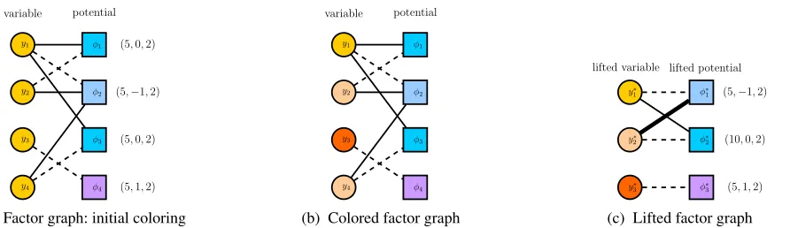
y1
y2
y3
y4
φ1
φ2
φ3
φ4 (5,0,2)
(5,−1,2)
(5,0,2)
(5,1,2)
variable potential
(a) Factor graph: initial coloring
variable potential
y1
y2
y3
y4
φ1
φ2
φ3
φ4
(b) Colored factor graph
y∗ 1
y∗ 2
y∗ 3
φ∗ 1
φ∗ 2
φ∗ 3
(5,−1,2)
(10,0,2)
(5,1,2) lifted variable lifted potential
(c) Lifted factor graph
Figure 1: The factor graph of the HL-MRF model presented in Example 1. The labels of the factor nodes appear on their right side. Edge weights are represented by line style (solid: 1, dashed: -1, thick: 2).
The function obtained by this method is also a HL-MRF en-ergy function. Preserving this form is crucial, since the effi-cient ADMM method introduced earlier is tailored for func-tions of this form. At the end of this section, we show that we can obtain the solution of the original problem by solv-ing the lifted problem and mappsolv-ing its solution back to the original space.
3.1
Lifted HL-MRFs (LHL-MRFs)
Our lifting method operates on afactor graph, which is a graphical representation of a HL-MRF energy function.
Definition 3 (Factor Graph). The factor graph of an
HL-MRF energy function is a graph G = (U, V, E)in which
there is a node uj ∈Ufor each variable yj(j= 1, . . . , n) and a node vi ∈V for each potential φi(i = 1, . . . , m). For each nonzero coefficient xij of variable yj in
poten-tialφi there is an edge eij ∈ E between uj and vi with
the weight xij. Each nodevi ∈ V is labeled by the tuple
(wi, ci, di).
Example 2. The energy function of the HL-MRF in Example 1 can be represented by the factor graph in Fig. 1a.
We will now describe a method that given the factor graph
Gof an energy functionf, produces a potentially smaller factor graphG0. Instead of solving the MAP inference prob-lem forf, one can solve the MAP inference problem for the functionf0represented byG0and map the solution back to the variables inf.
We first assign the initial colors to the nodes of G = (U, V, E). The nodes in V receive different colors based on their labels: Two nodes with labels (w1, c1, d1) and
(w2, c2, d2)receive the same initial color iffc1 =c2, w1= w2 andd1 = d2. All nodes in U receive the same color,
which is different from the colors of the nodes in V. We then run the color-refinement algorithm onG, which out-puts a stable bi-coloring CU
1, . . . , CpU for the nodes in U
and CV
1 , . . . , CqV for the nodes in V. To create the lifted
factor graphG0 = (U0, V0, E0), we first create a lifted vari-able nodeu0
k for every color classC U
k and a lifted factor
nodev0
lfor every color classClV. Each lifted variable node u0
k and lifted factor node v
0
l corresponds to a set of edges
inG, namely Ekl = {eij ∈ E : vi ∈ CV
l , uj ∈ C
U k }.
If Ekl is non-empty, we connect the nodes u0
k and vl0 in G0 by an edge with the weight(P
(i,j):eij∈Eklxij)/|C V l |.
Let I = {i : vi ∈ CV
l } and (w, c, d) be the label of
some v ∈ CV
l . We label the node vl0 ∈ V0 by the tuple
(P
i∈Iwi, c, d).
Example 3. The output coloring of the color refine-ment algorithm is shown in Fig. 1b. According to this coloring, the variables are partitioned into sets
{y1},{y2, y4},{y3} and the factors are partitioned into sets{φ2},{φ1, φ3},{φ4} . From the color classes of Ex-ample 2, we obtain the lifted factor graph of Fig. 1c which represents the function: f(yyy∗∗∗) = 5 max(−y∗
1 + 2y∗2 −
1,0)2+ 10 max(y∗
1−y2∗,0)2+ 5 max(−y∗3+ 1,0)2.
As noted before, the expression in the above example is essentially a weighted sum of hinge functions which has the exact same form as (4). This implies that the function rep-resented by the lifted factor graph can also be solved using ADMM. To map the solution of lifted problem back to the original space, we only need to assign the value of the repre-sentative variables of each lifting color class to all the vari-ables in that color class.
3.2
Correctness of the method
We now show that optimizing over the lifted function pro-duces the same objective value as optimizing the original function, and the optimal values of the variables in the orig-inal problem can be derived from their lifted counterparts. Our proof is based on an existing procedure for lifting the
Quadratic Programming(QP) problems (Mladenov,
Klein-hans, and Kersting 2017). We show that the MAP inference problem in HL-MRFs can be cast as a QP problem and that lifting this problem produces another QP which is equivalent to the function produced by our lifting method.
To write the objective function of the MAP inference in Equation 4 as a QP, we replace themaxfunctions by con-straints over auxiliary variablesψi:
minX
i wiψdi
i s.t., ψi≥
X
j
xijyj−ci∀i, yyy, ψψψ≥000
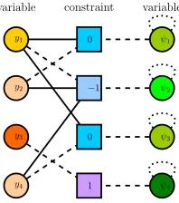
now explain how to construct the coefficient graph for (6) (for further details we refer to Mladenov, Kleinhans, and Kersting (2017)). The coefficient graph of (6) is the 4-tuple (U, V, Z, E)where the nodesuj ∈U,vi ∈U, andzi ∈Z
correspond to variable yj, constraint i, and variable ψi, re-spectively. For each nonzero coefficient xijthere is an edge with weight xij between the nodes uj and vi. For each constraint i, the nodes vi ∈V and zi ∈Z are connected by an edge with weight −ci, and if di = 2then there is a self-loop edge on ziwith the weight wi.
Initially all nodes in U ∪Z have the same color, which is not shared by any node in Z. Two nodes vi1, vi2 ∈ V
receive the same initial color iff ci1=ci2.
After performing the color refinement algorithm on this coefficient graph, the coefficient graph of the lifted QP problem is constructed by grouping the variables and con-straints of each color class together. The edge weights are aggregated in the same way as previously described in our method. The optimal value of a variable in the original QP is equal to the optimal value of its lifted counterpart.
y1
y2
y3
y4
0
−1
0
1
variable constraint
ψ1
ψ2
ψ3
ψ4 variable
Figure 2: The colored coefficient graph of the HL-MRF model presented in Example 1. Edge weights are represented by line style (solid: 1, dashed: -1, dotted: 5).
Example 4. The coefficient graph of the QP corresponding to Example 1 and the coloring assigned to it by the color refinement algorithm is presented in Fig. 2.
Assume that a functionf is lifted to another functionf0 using our proposed method. We demonstrate the correctness of our method by showing that the QP off can be lifted to the QP off0.
Theorem 1. Let G = (UG, VG, EG) be the factor
graph of an energy function of an HL-MRF, and Q =
(UQ, VQ, ZQ, EQ)be the coefficient graph of its QP. Then in the stable bi-colorings ofGandQ, the color classes ofU andV are the same.
Proof. Assume that in the stable bi-coloring CG of fac-tor graph G, the nodes are partitioned into disjoint colors
CG
1, . . . , CqG⊆VGandCqG+1, . . . , CqG+p ⊆UG. Let us
de-note byuG
j andvGi the nodes inGcorresponding to variable yj and factorφi in the HL-MRF energy function. Also let
uQj,v Q
i andz
Q
i denote the nodes corresponding to variable yj, constrainti, and auxiliary variableψiin the correspond-ing QP problem. We will now construct a stable bi-colorcorrespond-ing
CQof the coefficient graphQwith the following properties:
1) Variable nodes have the same color classes inCQandCG and constraint nodes inCQ have the same color classes as
factor nodes inCG, 2)CQis consistent with the initial color-ing ofQ, and 3)CQis the coarsest stable bi-coloring of the
graphQ. We first construct the coloringCQand then show how the above conditions hold for it. Let C(u)denote the color class of u in the coloring C. In CQ we assign the
colors to the nodes inUQ,VQ, andZQ based on the color
classes ofUGandVGin
CGas follows: uQj1 ∈ C
Q(uQ j2)⇔u
G j1 ∈ C
G(uG
j2) (7)
vQi1 ∈ C Q(vQ
i2)⇔v G i1 ∈ C
G(vG
i2) (8)
zQi1 ∈ C Q(zQ
i2)⇔v G i1∈ C
G(vG
i2) (9)
The first property holds by definition. By definition, the nodesuQj1, uQj2 ∈UQhave the same initial color iff the initial
colors of the nodesuG j1, u
G j2 ∈ U
G are the same. Similarly,
viQ1, viQ2 ∈ VQ receive the same initial color iff the nodes vG
i1, v G i2 ∈ V
G have the same initial color. Additionally, all
nodes in ZQ receive the same initial color. Hence
CQ is
consistent with the initial coloring ofQ.
To show that the coloring is stable, we need to show that the sum of edge weights connecting to the nodes in each color class is the same among all the nodes having the same color. So for each pair of variable nodes uQj1, uQj2 ∈ UQ
and color classClQ it should hold that uQj1 ∈ CQ(uQ j2) ⇔
P
i:vQi∈ClQxij1 =
P
i:vQi∈ClQxij2. SinceC
Gis a stable
col-oring ofGwe have uG j1 ∈ C
G(uG j2) ⇔
P i:vG
i∈ClGxij1 = P
i:vG
i∈ClGxij2 which together with equation 7 proves this
property. Similarly, for each pair of constraints i1, i2 and
color class CkQ it should hold that vQi1 ∈ C Q(vQ
i2) ⇔
P
j:uQj∈CkQxi1j=
P
j:uQj∈CkQxi2jwhich can be concluded
from equation 8 and the fact that vG
i1 ∈ C
G(vG i2) ⇔
P j:uG
j∈CkGxi1j = P
j:uG
j∈CkGxi2j. Note that the weights
of edges connecting to nodes ofψiare not included in these equations since ψi variables appear with the same coeffi-cient in all constraints. For a pair of nodesziQ1, z
Q
i2 ∈ Z
Q
wheredi1 = di2 = 1, we should have z Q i1 ∈ C
Q(zQ i2) ⇔ viQ1 ∈ C
Q(vQ
i2) which trivially holds according to
equa-tion 9. Finally, when di1 = di2 = 2, it should hold that ziQ1 ∈ C
Q(zQ i2)⇔v
Q i1 ∈ C
Q(vQ
i2)∧wi1 =wi2 which holds
according to equation 9 and the fact that ifwi1 6=wi2 then
the nodesvQi1, v Q i2 ∈V
Qare initialized with different colors.
Now what remains is to show thatCQ is the coarsest sta-ble coloring of graph Q, i.e., there is not another stable bi-coloring respecting the previous conditions that assigns fewer number of colors thanCQto the nodes ofQ. Assume
that there is a stable bi-coloringC0QofQwith fewer colors thanCQ. Then we can construct a stable bi-coloring
C0Gfor
the factor graphGthat respects its initial coloring, by par-titioning theUG andVG according to the color classes of UQ andVQ in
C0Q. Since partitions ofUQ andZQ are in
color classes inC0Qcan not be limited to color classes of the nodes inZQ. This means that
C0G has fewer color classes
thanCG, which is a contradiction.
4
Empirical Evaluation
In this section, we evaluate our proposed lifted inference al-gorithm, LHL-MRF, on various real and synthetic datasets. We investigate three research questions in our experiments:
Q1: How does lifting affect performance on real world datasets? Q2: How does the graph structure influence the impact of lifting?Q3:How much symmetry is required for lifting HL-MRFs to be effective? All experiments were run on a machine with 16GB RAM and an i5 processor. The im-plementations are all single-threaded. We implemented our models using the PSL open-source Java library1. We ground the rules using the PSL library and then run inference us-ing our own implementation of ADMM in C++2. Note that PSL removes a large number of trivial symmetries during the grounding process by removing trivially satisfied rules (for further information see (Augustine and Getoor 2018)). Removing these simple symmetries ensures the extra sym-metries that are obtained during our approach are non-trivial. We use Saucy3from theRELOOPlibrary to perform color
refinement (Mladenov et al. 2016).
Experiments on Real-world Data
We selected three real world datasets from different domains for which the corresponding PSL models have been used with promising results.
-Citeseer: This dataset includes 3312 papers in six cate-gories, and 4591 citation links. The goal is to classify doc-uments in a citation network. The original data comes from Citeseer . The details about the model and data can be found in Bach et al. (2017).
-Cora: This dataset includes includes 2708 papers in seven categories, and 5429 citation links. The goal is to classify documents in a citation network. The original data comes from Cora . The details about the model and data can be found in Bach et al. (2017).
-Wikidata: The dataset contains 419 families and 1,844 family trees. The goal is to perform entity-resolution on a family graph obtained form wikidata by crawling the site for familial relations. The details about the model and data can be found in Kouki et al. (2017).
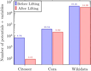
To address Q1, we measure the effects of lifting on the three datasets. Figure 3 presents the number of variables and potentials of these datasets before and after lifting. We ob-serve that there is a varying amount of symmetry in these datasets, the reduction in number of variables and potentials is about 20% in the Wikidata, 46% in the Cora, and 66% in the Citeseet dataset.
Table 1 shows the time to solve the original problem, i.e., HL-MRF, the time to solve the lifted problem, i.e., LHL-MRF (solving), the time to lift HL-LHL-MRF with the color re-finement algorithm, i.e., LHL-MRF (lifting), and the end
1https://github.com/linqs/psl 2
https://github.com/linqs/srinivasan-aaai19
3
http://vlsicad.eecs.umich.edu/BK/SAUCY
Datasets HL-MRF LHL-MRF LHL-MRF LHL-MRF (solving) (lifting) (total) (in sec) (in sec) (in sec) (in sec)
Citeseer 57.4 19.8 0.39 20.19
Cora 47.7 17.5 0.53 18.03
Wikidata 636.0 463.7 112.7 576.4
Table 1: Time taken to perform inference on different datasets.
Citeseer Cora Wikidata
102
103
104
105
106
107
8.76
10.54
15.21
4.41
9.92
14.98
Num
ber
of
poten
tials
+
variables
Before Lifting After Lifting
Figure 3: The number of variables and rules reduce in dif-ferent amount after lifting in real-world datasets.
to end inference time for the lifted approach, i.e., LHL-MRF (total) or LHL-LHL-MRF in short.
As expected, due to the large amount of reduction in the number of variables and potentials, there is a significant difference between the time taken for HL-MRF and LHL-MRF (solving) on all subsets. Even with a small 20% re-duction in number of variables and potentials in Wikidata, we see that LMRF (Solving) is 27% faster than HL-MRF and due to much higher reduction in other datasets, we see three-fold speed-ups in both the Cora and the Cite-seer datasets.
However, lifting time (LHL-MRF (lifting)) must also be considered. After accounting for this, we still see that LHL-MRF is about a 10% faster in the Wikidata dataset and al-most three times faster for the Cora and the Citeseer datasets when compared to HL-MRF.
10k 50k 100k 200k 500k 0
1 2 3 4 5
·105
10,629 50,413
1.01·105
2.01·105
5.02·105
6,641 25,886 49,116
92,457 1.9·105
Graph Density
Num
ber
of
poten
tials
+
variables
Before Lifting After Lifting
(a) For binary values, as the graph density in-creases, the total amount of lifting increases.
10k 50k 100k 200k 500k
1 1.5 2 2.5
Graph Density
Ratio
(full/lifted)
Binary 1 Decimal pt 4 Decimal pt
(b) For varying numbers of values, as graph density increases, the ratio of lifting varies.
10k 50k 100k 200k 500k
0 10 20 30 40
Graph Density
Time
(in
sec)
HL-MRF LHL-MRF(solving)
LHL-MRF LHL-MRF(lifting)
(c) Comparison of inferences times for HL-MRF and LHL-HL-MRF as graph density varies.
Figure 4: Comparison of inferences times and size of the problem for HL-MRF and LHL-MRF as graph density varies
We fix the number of users to1000, and randomly create friendship links between these users by varying the number of edges from10kto500k. In practice friendship is not nec-essarily a black-and-white matter, i.e., people can be friends to varying degrees. Hence, we consider three cases for the values of the friendship links: 1) binary values, 2) values between zero to one with one decimal point, 3) values be-tween zero to one with four decimal points. This means that friendship links can take only two values in the first case ({0,1}), 10 values in the second ({0.0,0.1, . . . ,1.0}) and 10,000 in the third case ({0.0000,0.0001, . . . ,1.000}). We randomly assign a label to users and keep 50% of the labels as evidence and another 50% as unknowns to be inferred. Figure 4a shows the total number of variables and poten-tials before and after lifting for the binary case. Figure 4b shows the ratio between the number of variables and poten-tials before and after lifting, for varying value ranges. We see that for the binary case, the amount of lifting is maxi-mized and the ratio increases as the graph density increases. However, as the value range increases, the amount of lifting drops significantly, and eventually there are no symmetries to be exploited. Finally, Figure 4c presents the processing time to solve the binary case. The results indicate that us-ing LHL-MRF gives a significant performance improvement over HL-MRF as the graph becomes denser. These results imply that there are complex trade-offs between the struc-ture of the graph and the range of the values in the data. We utilize exact lifting and therefore, we observe that LHL-MRF performs well for finding symmetries in datasets with denser structures and smaller range of values.
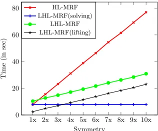
Finally, to further understand how the amount of sym-metry affects the overall inference time in a slightly more complex and realistic setting (yet still a synthetic dataset), we study the social affiliation dataset and the PSL model used by Bach et al. (2017) for scalability analysis. We use a dataset that contains 22k nodes and 130k edges4.
We begin by lifting this dataset to remove all symmetry (the original dataset has less than 1% symmetry). To induce
4
https://github.com/stephenbach/admm-speed-test
symmetry, we systematically inject the same structure to the data. This is done by duplicating every grounded rule and shuffling the data. We duplicate the grounded rules up to 10 times creating 10 subsets (named 1x, 2x, 3x..., 10x), where the 10x subset has 10 times as many potentials created by duplicating the original data i.e., the 1x subset.
1x 2x 3x 4x 5x 6x 7x 8x 9x 10x 0
20 40 60 80
Symmetry
Time
(in
sec)
HL-MRF LHL-MRF(solving)
LHL-MRF LHL-MRF(lifting)
Figure 5: As symmetry increases, the gap between time solv-ing HL-MRF and LHL-MRF increases.
Figure 5 shows the results of HL-MRF and LHL-MRF (split into LHL-LHL-MRF (solving), LHL-LHL-MRF (lifting), and LHL-MRF on all 10 subsets. For the smallest dataset (which contains no symmetry), the time required for LHL-MRF is higher than HL-LHL-MRF due to the time taken to per-form lifting. However, increasing the size of the dataset from two to ten, we observe that the amount of time taken by LHL-MRF to solve the problem is getting much lower than HL-MRF. It is noticeable that as the symmetry increases, the gap between solving HL-MRF problem and LHL-MRF problems widens. Note that the inference time in LHL-MRF for all 10 subsets is the same (equal to 1x dataset), which is the flat line in Figure 5 for LHL-MRF (solving).
1x 2x 3x 4x 5x 6x 7x 8x 9x 10x
101
102
103
104
105
106
Symmetry
Log
of
Time
(in
sec
)
HL-MRF HL-MRF(Gurobi)
LHL-MRF LHL-MRF(Gurobi)
Figure 6: As symmetry increases, the gap between time solving HL-MRF and HL-MRF(Gurobi) increases expo-nentially. The difference between MRF and LHL-MRF(Gurobi) remains the same as the 1x dataset.
versions which use Gurobi– an off-the-shelf commercial QP solver–. We denote these methods which use Gurobi HL-MRF (Gurobi) and LHL-HL-MRF (Gurobi). For all 10 subsets, we observe that using HL-MRF and LHL-MRF consistently and significantly outperforms HL-MRF (Gurobi) and LHL-MRF (Gurobi) respectively. We also see that this difference increases as the size of the data increases. Note that the time taken to solve using LHL-MRF (Gurobi) is similar to other lifting methods such as belief propagation. For most of the lifting methods, the time complexity grows cubicly with the number of variables in the data. However, our approach is unique and desirable as it maintains the original form of the function allowing us to use ADMM which is known to be much more scalable than other approaches (Forouzan and Ihler 2013).
To our best knowledge, the size of datasets used in other lifted inference papers are in order of 1000s of variables and potentials, whereas using ADMM in our approach allow us to easily scale to problems with millions of variables and potentials.
5
Discussion and Future Directions
We have shown that there are significant opportunities for lifted inference, even in the case where we have continuous-valued variables defined by HL-MRFs. Through empirical evaluation on real datasets, we show that the inference task for HL-MRF models can run up to three times faster by us-ing MRFs. However, it is important to note that LHL-MRFs cannot guarantee speed-ups for all types of problems. We investigate the effects of graph density and range of real values on lifting in HL-MRFs. However, studying the char-acteristics of the optimization problem after lifting is left for future work. We also notice that on small sized problem, in which inference takes less than one second to finish in HL-MRFs, the overhead of lifting is noticeable, and there-fore even with a huge amount of reduction in the number of variables and potentials, we cannot necessarily reduce the solving time of LHL-MRFs.This work suggests other interesting directions for future
work. First, in this work we only exploit exact symmetries, which may be hard to find in some applications. Previous work indicates approximate lifted inference can improve the performance without compromising on other metrics like precision (Sen, Deshpande, and Getoor 2009). In our setting, approximate lifting could also lead to a greater reduction in number of variables and speed up the task of inference. Sec-ond, two of the most challenging tasks in MRFs are learning the weights and the structure of the logical rules from the data. Structure learning and weight learning are often per-formed using a scoring function that iteratively uses a MAP state. An interesting path to explore is to employ lifted in-ference to make such systems more efficient.
6
Conclusion
In this paper, we introduced LHL-MRF, a novel approach to lifted inference in HL-MRFs. LHL-MRF marries the pow-erful ideas of lifted inference with the color refinement al-gorithm of Grohe et al. (2017) with the convex inference approach proposed by Bach et al. (2017), to solve large-scale graphical models described by HL-MRFs. By combin-ing these two ideas, our method is able to reduce the num-ber of variables and potentials in a model and perform infer-ence efficiently on a significantly smaller optimization prob-lem. Through empirical evaluation, we show that the infer-ence task for HL-MRF models on relatively small real world problems can be made to run three times faster. Further, in our experiments, we investigated how varying symmetry af-fects the performance of LHL-MRF and we explored the im-pact of both structure and domain values on the efficiency of LHL-MRF.
Acknowledgement
We would like to thank Kristian Kersting for his construc-tive feedback and the anonymous reviewers for their helpful suggestions. This work is supported by the National Science Foundation under grant numbers CCF-1740850 and IIS-1703331, and by the US Army Corps of Engineers Research and Development Center under contract number W912HZ-17-P-0101. Behrouz Babaki is supported by a postdoctoral scholarship from IVADO through the Canada First Research Excellence Fund (CFREF) grant.
References
Aditya, S.; Yang, Y.; and Baral, C. 2018. Explicit reason-ing over end-to-end neural architectures for visual question answering. InAAAI.
Alshukaili, D.; Fernandes, A. A. A.; and Paton, N. W. 2016. Structuring linked data search results using probabilistic soft logic. InISWC.
Augustine, E., and Getoor, L. 2018. A comparison of bottom-up approaches to grounding for templated Markov random fields. InSysML.
Beltagy, I.; Erk, K.; and Mooney, R. J. 2014. Probabilistic soft logic for semantic textual similarity. InACL.
Boyd, S. P.; Parikh, N.; Chu, E.; Peleato, B.; and Eckstein, J. 2011. Distributed optimization and statistical learning via the alternating direction method of multipliers.Foundations and Trends in Machine Learning.
Chavira, M., and Darwiche, A. 2008. On probabilistic in-ference by weighted model counting. Artif. Intell. 172(6-7):772–799.
Chen, P.; Chen, F.; and Qian, Z. 2014. Road traffic con-gestion monitoring in social media with hinge-loss Markov random fields. InICDM.
Codenotti, P.; Katebi, H.; Sakallah, K. A.; and Markov, I. L. 2013. Conflict analysis and branching heuristics in the search for graph automorphisms. InICTAI.
De Raedt, L., and Kersting, K. 2011. Statistical relational learning. InEncyclopedia of Machine Learning. Springer. de Salvo Braz, R.; Amir, E.; and Roth, D. 2005. Lifted first-order probabilistic inference. InIJCAI.
Dechter, R., and Mateescu, R. 2007. AND/OR search spaces for graphical models. Artif. Intell.171(2-3):73–106. den Broeck, G. V.; Taghipour, N.; Meert, W.; Davis, J.; and Raedt, L. D. 2011. Lifted probabilistic inference by first-order knowledge compilation. InIJCAI.
Deng, L., and Wiebe, J. 2015. Joint prediction for entity/event-level sentiment analysis using probabilistic soft logic models. InEMNLP.
Ebrahimi, J.; Dou, D.; and Lowd, D. 2016. Weakly super-vised tweet stance classification by relational bootstrapping.
InEMNLP.
Forouzan, S., and Ihler, A. 2013. Linear approximation to admm for map inference. InJMLR W&CP, 48–61.
Getoor, L., and Taskar, B. 2007. Introduction to statistical relational learning. MIT.
Gogate, V., and Domingos, P. M. 2010. Exploiting logical structure in lifted probabilistic inference. In StarAI Work-shop at AAAI.
Gridach, M.; Haddad, H.; and Mulki, H. 2017. Churn iden-tification in microblogs using convolutional neural networks with structured logical knowledge. In NUT workshop at
EMNLP.
Grohe, M.; Kersting, K.; Mladenov, M.; and Schweitzer, P. 2017. Color refinement and its applications. In Van den Broeck, G.; Kersting, K.; Natarajan, S.; and Poole, D., eds.,
An Introduction to Lifted Probabilistic Inference. Cambridge University Press.
Kazemi, S. M., and Poole, D. 2016. Knowledge compilation for lifted probabilistic inference: Compiling to a low-level language. InKR.
Kersting, K.; Ahmadi, B.; and Natarajan, S. 2009. Counting belief propagation. InAUAI, 277–284.
Kersting, K. 2012. Lifted probabilistic inference. InECAI. Kimmig, A.; Mihalkova, L.; and Getoor, L. 2015. Lifted graphical models: a survey.Machine Learning99(1):1–45.
Kouki, P.; Pujara, J.; Marcum, C.; Koehly, L. M.; and Getoor, L. 2017. Collective entity resolution in familial networks. InICDM.
Lalithsena, S.; Perera, S.; Kapanipathi, P.; and Sheth, A. P. 2017. Domain-specific hierarchical subgraph extraction: A recommendation use case. InBigData.
Mladenov, M.; Ahmadi, B.; and Kersting, K. 2012. Lifted linear programming. InAISTATS.
Mladenov, M.; Heinrich, D.; Kleinhans, L.; Gonsior, F.; and Kersting, K. 2016. Reloop: A python-embedded declarative language for relational optimization. In DeLBP Workshop at AAAI.
Mladenov, M.; Kersting, K.; and Globerson, A. 2014. Effi-cient Lifting of MAP LP Relaxations Using k-Locality. In
AISTATS.
Mladenov, M.; Kleinhans, L.; and Kersting, K. 2017. Lifted inference for convex quadratic programs. InAAAI.
Poole, D. 2003. First-order probabilistic inference. InIJCAI. Ramana, M. V.; Scheinerman, E. R.; and Ullman, D. 1994. Fractional isomorphism of graphs. Discrete Mathematics. Richardson, M., and Domingos, P. M. 2006. Markov logic networks. Machine Learning62(1-2):107–136.
Sen, P.; Deshpande, A.; and Getoor, L. 2009. Bisimulation-based approximate lifted inference. InUAI.
Singla, P., and Domingos, P. M. 2008. Lifted first-order belief propagation. InAAAI.