Algorithm for Dynamic Formation of Condition Equations in N-Dimensional Network

(1)

Algorithm for Dynamic Formation of

Condition Equations in N-Dimensional

Network

C. P. E. Agbachi

Department of Mathematical Sciences, Kogi State University Anyigba, Kogi State, Nigeria

Abstract— Condition equations, once used to be the only viable and memorable option in the model of computation by least squares estimation. That was in the early days of computing when RAM size of machines was in the region of 128K and search for models with efficient use of memory was imperative. Even today the merits of condition equations remain patent. The drawback has always been the ability to form the prerequisites in the first place. This paper discusses versatile algorithms for automatic generation of condition equations, and in the process restoring the model as a utility in resolving networks in Geomatics Engineering.

Keywords—Levels, Traverse, GPS, Cycles, Graph, BFS, DFS, Span Tree.

I. INTRODUCTION

Condition equations arise out of geometric considerations that result from evaluating internal and external consistency in a survey network.A case in point is one dimensional situation where Y is a measurable variable and of the form Y = {ΔH}.

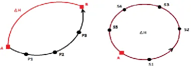
Fig. 1 Consistency in Networks

In Fig.1 is an illustration of closures in networks. The first involving a survey from A to B, fixed stations, should be in agreement with existing framework. On the second option, the internal consistency where the survey starts from and ends at the same point A, ought to be satisfied.

Enumerating in each case, there is one condition equation to fulfil:

hB – hA = ΔH and ΔH = 0 Thus in simple adjustment process, the errors are spread equally between the observed stations. This

translates into proportional distribution of closures over the number of stations for final values of computed positions.

A. Least Squares Approach

A rigorous solution by least squares method is available, based on condition equations. It is the option in cases of over determined equations.

Fig. 2 Residuals

Imagine measured points YM as in the diagram

Fig. 2, where YP are the most probable values such

that the residual 𝜗 = 𝑌𝑃− 𝑌𝑀 --- (1)

Then if there are s observed quantities and r condition equations, r<s, the linear relationship may be expressed as follows:

𝑎11𝑌𝑃1 + 𝑎12𝑌𝑃2 + ⋯ +𝑎1𝑠𝑌𝑃𝑠= 𝐶1

𝑎21𝑌𝑃1 + 𝑎22𝑌𝑃2 + ⋯ +𝑎2𝑠𝑌𝑃𝑠= 𝐶2

⋮ ⋮ ⋮ 𝑎𝑟1𝑌𝑃1 + 𝑎𝑟2𝑌𝑃2 + ⋯ +𝑎𝑟𝑠𝑌𝑃𝑠= 𝐶𝑟

The above equations are idealistic in nature. In the field, the measurements form the basis of adjustment computations. Hence substituting for

𝑌𝑃 = 𝜗 + 𝑌𝑀,leads to A𝝑 = b --- (2)

Minimising 𝝑TW𝝑 is equivalent to minimising

𝝑T

W𝝑 -2(A𝝑- b)Tk, where k is the r x 1 matrix of

Lagrange coefficients. This leads to 𝝑 = W

-1

ATk.With k = (AW-1AT)-1b as in [1], the resulting solution is 𝝑 = W-1AT(AW-1AT)-1b --- (3)

(2)

Taking the models described in Fig 1, it is easy to verify that a solution exists by method of least squares condition equations. Consider the case of internal consistency where a survey starts from Station A and closes at the same point in a levelling process.

The measurements are h1, h2, … , h6 and by

arguments in (1),𝜗 = ℎ𝑃− ℎ𝑀. Thus as in (2)

(1, 1, 1, 1, 1, 1) 𝑣1

𝑣2

𝑣3

𝑣4

𝑣5

𝑣6

= ΔH

Let W = I, then (3) reduces to 𝝑 = AT(AAT)-1b.

Hence

𝑣1

𝑣2

𝑣3

𝑣4

𝑣5

𝑣6

= ΔH 6 ΔH 6 ΔH 6 ΔH 6 ΔH 6 ΔH 6

And the result is ℎ𝑃 = 𝜗 + ℎ𝑀 which

corroborates the proportional distribution of errors in cases of one condition equations.

Fig. 3

In general, surveys involve networks where several conditions arise. In Fig 3for instance there are four cycles for bases of condition equations.

Fig. 4 Survey Network

While the number of conditions can be obvious by inspection, Fig. 3, it is not always clear in large

survey networks, as in Fig. 4. Hence, the search is necessary for a suitable algorithm.

II. GRAPH ALGORITHMS

Fig. 5

A graph, Fig. 5, is a data structure important in representing information with regards to patterns, directions and in effect, networks. By definition, a graph comprises of nodes and connections known as edges. Where directions define the edges, it is known as a Digraph. Along with weighted graphs, they find common applications in Geoinformatics.

Trees and graphs are complements to each other. A tree is a connected graph without cycles. Similarly, a graph is a free tree, a tree without root. Traversal routines exist to transform graphs into spanning trees and vice versa. This is particularly useful when processing fundamental cycles [2], in order to establish condition equations.

A. Cycle Processing

By description a graph maybe defined as acyclic [3], meaning there are no cycles. However in context of survey applications, the emphasis is on adaptation, recognition of geometry and topology. Therefore, a cycle or loop starts from a node, passing through other nodes and terminating at the start node. Thus, while Fig. 3 may represent a DAG, the entities, Loop 3 etc. can be reduced to cycles by reversing observed directions in affected segments.

Processing cycles starts with a spanning tree and addition of cross or back edges. The key algorithms are Breadth First Search and Depth First Search [4].

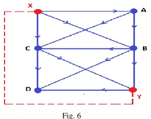
Fig. 6

(3)

terminates like wise. Thus, observed directions are important in computations and are reflected in processing algorithms. With respect to the model, the survey involves transfer of position from X, proceeding and closing at Y. Further observationsallow determination of C and D, to complete the network as a connected graph.

1. Breadth First Search:

Breadth First Search starts by investigating each direction emanating from X, the first station. It then moves to next layer, the next station B until finally all the nodes are connected in a spanning tree, Fig 7.

Fig. 7

Next fundamental cycles are constructed by adding cross edges. There are 5 cycles where the fifth, XBYX ensures consistency with external framework.

2. Depth First Search:

Depth First Search, operating from the first station X follows a one-way route in the main direction of survey, until the last stop D, when there is no further path to proceed. It then retraces its way backwards to investigate unexplored routes, BC, until completion that leads to a spanning tree, Fig 8.

Fig. 8

Back edges are then fitted to construct fundamental cycles, in order to establish the condition equations. These cycles are: XABX, ABCA, BYCB, YDCY, and XBYX.

3. Model Solution:

A model solution arises out of comparison of the two search options, BFS and DFS. The consensus of opinion is that choice depends on the nature of data structure. In this regard, a survey route is characterized by depth and DFS is a natural representation. Furthermore, it does not entail huge memory requirements.

BFS nevertheless has advantage of minimum path length in cycle formation. Involving cross edges, the cycles have less overlap and agrees more readily with visual observations of geometry. However it does not lend with run of survey and topology.

Generally, as described in [5], the best option is offered by Depth - Limited Search, which is to say that thefinest solution lies in improving DFS. Thus, in this application, DFS is adopted and have proved very robust and reliable.

III.CONDITION EQUATIONS

Condition equations can be developed from the cycles formed in Fig. 8. Considering in the first instance a case of one-tuple, V = {H}, the equations are as follows:

𝐻𝑋𝐴 +𝐻𝐴𝐵-𝐻𝑋𝐵 = 0

𝐻𝐴𝐵 + 𝐻𝐵𝐶-𝐻𝐴𝐶 = 0

𝐻𝐵𝑌-𝐻𝐶𝑌-𝐻𝐵𝐶 = 0

𝐻𝑌𝐷-𝐻𝐶𝐷 + 𝐻𝐶𝑌 = 0

𝐻𝑋𝐵 + 𝐻𝐵𝑌 +𝐻𝑌𝑋 = 0

where𝐻𝐴 is the MPV and𝐻𝑋𝐴 = 𝐻𝐴 − 𝐻𝑋 .

Continuing as in (1),

𝑣𝐻_𝑋𝐴 + 𝑣𝐻_𝐴𝐵-𝑣𝐻_𝑋𝐵 = 𝐶1

𝑣𝐻_𝐴𝐵 + 𝑣𝐻_𝐵𝐶-𝑣𝐻_𝐴𝐶 = 𝐶2

𝑣𝐻𝐵𝑌 -𝑣𝐻𝐶𝑌-𝑣𝐻𝐵𝐶 = 𝐶3 𝑣𝐻_𝑌𝐷-𝑣𝐻_𝐶𝐷 + 𝑣𝐻_𝐶𝑌 = 𝐶4

𝑣𝐻𝑋𝐵 + 𝑣𝐻𝐵𝑌 + 𝑣𝐻𝑌𝑋 = 𝐶5

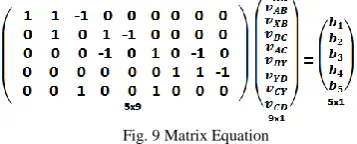
In matrix format, A𝝑 = b and the expression is:

Fig. 9 Matrix Equation

It may be noted that in equation C5, YX is a fixed

line, and therefore a residual correction𝑣𝐻𝑌𝑋is not

(4)

A. N-Dimensional Network

Traversing is one of the most versatile and common means of establishing a control network [6]. Invariably, the mode of collection is automated and standard setting is usually three dimensions.

Computations of traverse survey always start with determining provisional positions. These are subject to further computations, an adjustment process for final results. Thus, irrespective of the mode of estimation, derived positions are available to check for internal and external consistency in geometry. And it would be more expedient to continue with determining the most probable values by least squares method of condition equations.

With reference to Fig. 8, a three dimensional network may be considered. It could be noted as in Fig. 1 that where there are sub stations, it would be more efficient to obtain the results in a secondary process by proportional error distribution. Hence this adjustment is in respect of primary nodes in the network, Fig. 6.

Fig. 10 3-D Matrix Equation

The cycles in Fig. 8, form the basis of a three dimensional condition equations. It involves constructing a matrix as in Fig. 9, with each representing a dimension. As in Fig. 10 therefore, there are three partitions for Easting, Northing and Height. Solution then follows the form of equation 3 and when it comes to covariance matrix, a weight scheme W, based inversely on number of sub stations is reliable. Error estimates may be obtained from 𝐐_𝒍 = 𝐐𝒍[ 𝐈- 𝐁𝐓 (𝐁𝐐𝒍𝐁𝐓) −𝟏𝐁𝐐𝒍] as in [7].

Thus networks of the form in Fig. 4 are ideally computable.

IV.PROGRAMMING

Programming in early days was based on the principle of information processing. The evolution today is knowledge processing embodying Artificial Intelligence. Thus, the current techniques require knowledge representation of human taught processes by method of engineering [8, 9].

A. Knowledge Representation

The purpose of knowledge representation is to encompass the descriptions of a network in a suitable variable. Since a digraph describes a survey network, that process requires graph data structures. Thus, a single program variable representation could hold all observations and description of a network.

In this context, while frames are a form of knowledge representation, object constructs are the implementation platforms [10, 11]. The start to this construction is with node stations and the edges that provide the path links.

1. Node Object:

Fig. 11 Node Object

The node object, Fig. 11, starts with composition of record information. This record applies to every station in the network and thus covers requirements for sub stations, and results during computation.

Fig. 12 Node Definition

A node may be described with respect to graph structure, as the station where the sum of In-degree or Out-degree is greater than one, Fig 12. The fields within the records therefore have this variable provision. Other complements include reference and forward paths for describing instances in a traverse network.

(5)

2. Edge Object:

Fig. 13 Edge Definition

The edge object follows the same pattern with node object by construction of record information. Important to note are the variables, FromStn and ToStn. They designate the direction of the edge in the diagraph, such as BA, BC and DC in Fig 12. Also of note is the number of setups that constitute the weights for each edge, useful in adjustment computations in the network.

Similarly, the Boolean variables, Open, Ticked, Marked and Status play key roles in monitoring paths that need to or have been processed during formation of a span tree. Equally, the sign variable serves the useful purpose of reversing observed direction during construction of fundamental cycles.

3. Network Object:

The network object is the next logical construction. This is in form of variable definition of a survey network, irrespective of size or dimension.

Fig. 13 Network Definition

Of note are the variables, EdgeList and NodeList for storage mechanism. This is in preference, being more suitable to such options as Adjacency Matrix.

The methods FormNodes, LinkNodes provide a mapping description of the network. Add_PrvCoords provides preliminary positions and SaveData, saves the network to file for use in generating cycles and least squares computation.

B. Cycle Generation

In earlier discussions, the DFS was demonstrated as a more suitable algorithm for cycle processing. However, for implementation the mechanism differs from standard approach involving stacks etc. Rather what is adopted in this instance is analternative to suit survey applications.

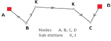
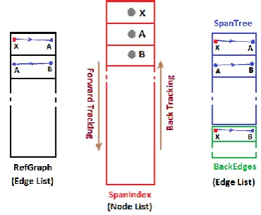
Fig. 14 Program Steps

With respect to Fig. 6 representing the network, a program implementation is described with illustrations in Fig 14. Thus, RefGraph is a variable representation for the structure as edge list. The same form applies to SpanTree and BackEdges. SpanIndex is a node list.

The process starts with initialization where SpanIndex, SpanTree are empty. The first segment XA, invariably the origin of the survey is evaluated and inserted into SpanTree. At the same time, the nodes X and A are inserted into SpanIndex. The target station A becomes the reference in forward tracking that yield the edge AB. Both the SpanIndex and SpanTree are subsequently updated. Forward tracking continues until a leaf, D, is encountered. Back tracking then follows until B is accessed and a new segment BC is found and explored, Fig 8.

(6)

Fig. 15Cycle Object

The programming implementation of this construction can be achieved by Cycle object, Fig. 15. Of note are the fields that include refGraph, SpanIndex, SpanTree etc. The key methods are CreateASubTree and BuildTheLoops.

1. Create A Sub Tree:

procedureTCycle.CreateASubTree; begin

New(SpanIndex, Init(500,50)); New(SpanTree, Init(500,50)); New(refGraph, Init(500,50)); TransferEdges;

FormSpanTree; FindBackEdges; AddCtrlEdges; SaveTree; end;

Fig. 16

Create a sub tree begins with initialization to create SpanIndex, SpanTree and refGraph. Thereafter, TransferEdges builds a copy of the network in refGraph, an edge list structure. FormSpanTree then executes to create a SpanTree.

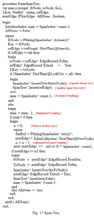
SpanTree in Fig. 17 starts after initialization, by constructing the first segment of the DFS spanning tree. Accordingly, reference and target nodes are registered in Node List. The outbound search for the next segment then begins with:

frNode := PString(SpanIndex^.At(num))^;

Key :=frNode;refEdge := refGraph^.FirstThat(@Search);

Operating in a repeat loop, the search moves in a forward direction, updating the Node List and SpanTree. When a leaf is encountered, back tracking commences with num := num -1.

At a stage the tracking returns to the root node from where forward search resumes for inbound observations. It executes inside a repeat loop untilsearch is exhausted and no further edges are detected. AllDone is then flagged true and the construction is complete.

Fig. 17 Span Tree.

The routine concludes with FindBackEdges, constructing the back edges. This is derived from the main graph as missing links in the spanning tree. By expression: BackEdges = refGraph – SpanTree.

In the same measure, AddCtrlEdges adds the external links in the network to a common list database, CycleIndex.

2. Build The Loops:

procedureTCycle.BuildTheLoops; begin

FetchBackEdges; :

ConstructCycles; LoopClosure; SaveCycles;

end;

(7)

Next a similar exercise obtains a list of back edges to enable construction of cycles to begin.

Fig. 18

The process ConstructCycles, Fig. 18, starts with initialisation, creating a segment list for each cycle, and setting LoopCount and g to zero. The variable ref stores the first back edge, and that is followed by insertion into Segments list. Trace then searches for other segments to make up the cycle. If on Target is true, the search is successful and a Loop object is formed. It may be noted how closures de, dn, dh in the cycle and linear accuracy are determined during initialization. The routine operates in a repeat loop until all the back edges are used in forming fundamental cycles in the network.

Condition equations can then follow as described in Figs. 8, 9 and 10.

V. APPLICATION

The application of this algorithm has proved very successful [12] in level and traverse networks.

A. Level Network

There are two considerations for illustration, namely description of the network and cycles in the network. It involves a large field survey.

1. Description:

Description starts with the edges, runs in the survey network. Each run has a source and terminating node. Also the edges are weighted with such information as number of setups and height difference, Fig. 19. There are about 311 edges in the survey network.

The node details complement the edge

description. There are 122 stations with in and out degrees at each station. The provisional heights complete the information to provide a picture of the network.

Fig. 19

2. Cycles:

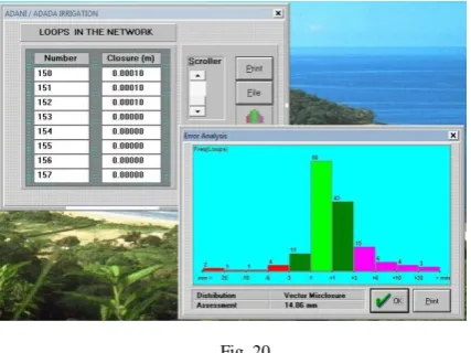
Cycle formation is the next logical step that follows the descriptions. This is illustrated in fig. 20.

Fig. 20

It involves as many as 158 cycles and requiring same number of condition equations. A button lists the segments in each cycle while histogram is also available to show the spread of closures for analysis.

B. Traverse Network

Traverse network is also modelled on descriptions and cycles in the network. This illustration involves a 3-D survey comprising 15 stations.

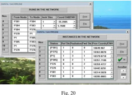
1. Description:

(8)

Fig. 20

Node details include instances as reference and forward stations in the network. The number of radiations is available to assist reconstruction of the network. Often field topology may differ from design and this facility is useful. The computed provisional coordinates are also available for determining closures in the survey.

1. Cycles:

Fig. 21

There are six cycles in the network with closures and linear accuracy as illustrated in each case, Fig 21. A List button generates the segments in each cycle. The six cycles lead to formation of 18 condition equations for a 3-D network.

VI.CONCLUSION

It is generally accepted of the need for checks on consistency in networks prior to computations. Even in the much acclaimed parametric model of least squares adjustment, provisional coordinates are prerequisites to computations, such that an obvious complement is to profile resultant closures and linear accuracies in the network. Hence, the next logical step would be to incorporate cycle processing in the algorithm.

Survey instruments continue to evolve and in the current model of Total Stations, options exist for observations in coordinate mode. And if this option is hardly taken, it is because of issues of computability, because most software packages would rather process inputs involving direct observables, angles and distances. In this paper, the constraints have been removed. As such coordinate observations directly measured by Total Stations and GPS can be computed to the same standard as in precise level network. That is in n-dimensions, by least squares methodof condition equations.

Condition equations have always been preferred for safeguards that are inherent in use and memory efficiency. This paper has restored it for ascent, appreciation and as a ready complement in resolving survey networks.

REFERENCES

[1] M. A. R. Cooper,“Fundamentals of Survey Measurement and Analysis”, Granada, 1982.

[2] Donald E. Knuth, “The Art of Computer Programming, Vol. 1 (3rd_{Edition): Fundamental Algorithms”, Addison}

Wesley Longman Publishing Co.

[3] Paul Van Dooren, “Graph Theory and Applications”, Université Catholique de Louvain, Belgium. Dublin, August 2009.

[4] Jean-Paul Tremblay, Paul G. Sorenson, “An Introduction to Data Structures With Applications”, McGraw Hill Computer Science Series 2nd Edition.

[5] R. C. Chakraborty, “Problem Solving, Search and Control Strategies: AI Course Lecture 7-14”,RC Chakraborty,2010, www.myreaders.info

[6] Yuji Murayama Surantha Dassanayake, “Fundamentals of Surveying Theory”,Division of Spatial Information Science, University of Tsukuba.

[7] M. A. R. Cooper, “Control Surveys in Civil Engineering”, Collins 1987.

[8] C. P. E. Agbachi, “Optimisation of Least Squares Algorithm: A Study of Frame Based Programming Techniques in Horizontal Networks”, IJMTT, Volume 37 Number 3 - September 2016.

[9] C. P. E. Agbachi, “Design and Application of Concurrent Double Key Survey Data Structures”, IJCTT, Volume 36 Number 3 - June 2016.

1995-2016. http://www.marcocantu.com/objectpascal [12] C. P. E. Agbachi, “Surveying Software”, Chartered