Liu Estimates and Influence Analysis in Regression Models with Stochastic Linear Restrictions and AR (1) Errors

Liu Estimates and Influence Analysis in Regression

Models with Stochastic Linear Restrictions and AR (1)

Errors

H. Mohammadi and A. R. Rasekh

*

Department of Statistics, Faculty of Mathematical Sciences and Computer, Shahid Chamran University of Ahvaz, Ahvaz, Islamic Republic of Iran

Received: 17 February 2019 / Revised: 27 April 2019 / Accepted: 26 May 2019

Abstract

In the linear regression models with AR (1) error structure when collinearity exists,

stochastic linear restrictions or modifications of biased estimators (including Liu

estimators) can be used to reduce the estimated variance of the regression coefficients

estimates. In this paper, the combination of the biased Liu estimator and stochastic

linear restrictions estimator is considered to overcome the effect of collinearity on the

estimated coefficients. In addition, the deletion formulas for the detection of influential

observations are presented for the proposed estimator. Finally, a simulation study and

numerical example have been conducted to show the superiority of the proposed

procedures.

Keywords: Liu estimator; Linear stochastic restrictions; Collinearity; Autocorrelated error; Influence analysis.

* _{Corresponding author: Tel: +986133331043; Fax: +986133331043; Email: [email protected]}

Introduction

The problem of collinearity in regression models refers to the situation where the explanatory variables have the near-linear dependency. By considering independent and identically distributed errors (homoscedasticity), it is well known that the ordinary least squares estimators (OLSE) are unbiased and have minimum variance in the class of linear unbiased estimators. However, in the presence of collinearity, they are no more reliable estimators, [1,2]. Collinearity causes the variance of the estimates to be large, and so the estimates of parameters will be unstable. To overcome this problem, one way is to make use of prior knowledge of observations and to deal with this information as linear stochastic restrictions. In such a case, the mixed estimators proposed by Theil and

Goldberger [3] and Theil [4] can be used, which is gained by unifying the sample and the prior information.

The other remedy to combat the collinearity problem is to use biased estimators such as the popular ridge estimator [5]. In 1993, Liu [6] introduced a new biased estimator called the Liu estimator by combining the Stein estimator [7] and the ridge estimator and showed that it can be superior over each of them in the MSEM sense. He also pointed out that it is easier to choose the Liu biasing parameter than to choose that of the ridge estimator since the Liu estimator is a linear function of its biasing parameter, but the ridge estimator is a complicated function of it.

assumption of homoscedasticity by combining the mixed estimator and the ridge estimator. Also, Hubert and Wijekoon [9] introduced the stochastic restricted Liu estimator under the same assumption and Yang and Xu [10] introduced another stochastic restricted Liu estimator by combining them in an alternative way.

In practice, the assumption of independent and identically distributed errors (homoscedasticity) does not always hold. Sometimes the data are collected over time and so cause the errors to be correlated. A commonly occurring case is when the errors follow a 1st

order autoregressive process (AR(1)). In such cases fitting an inappropriate model can have deleterious effects. A classic example can be found in Box and Newbold [11] who commented on a paper by Coen et al. [12]. The latter seemingly showed that car sales seven quarters earlier could be used to predict stock prices. But they failed to examine residuals and there was strong evidence that the errors were correlated. After fitting an appropriate model, Box and Newbold showed that there was no significant relationship between the two variable [13]. In fact, in practical applications, the neglect of such correlation in the errors may lead to inefficient parameter estimates and misleading inferences from hypothesis tests and inefficient predictions. The reason is that the OLSEs fail to achieve minimum variance estimates and the usual estimator of the variance-covariance matrix will be biased (see Griffith et al. [14]). To overcome these effects of autocorrelation, Aitken [15] proposed the generalized least squares estimator (GLSE). However, the presence of collinearity in the regression models with AR(1) error, will also result in unreliable GLS estimates, because of the large total variance. So these two problems should be examined simultaneously in order to achieve an appropriate estimation procedure for regression coefficients. The interested reader may refer to [16-20] for more details.

On the other hand, all the observations do not have the same impact on the estimated regression coefficients or on the resulting fitted values, therefore after fitting a regression model and using an estimation procedure to understand the relationship between variables, it is important to detect influential observations and (or) outliers in the framework of influence analysis. There are different statistical measures to detect these potentially influential observations, some of which are based on deleting cases. For example, the influence function for ith observation can be obtained as differences between the parameter estimated with and without the ith observation. The limitation of this approach is that it cannot be easily generalized to the linear regression model with 1st _{order autoregressive}

errors, in which the dependency structure of the autoregressive model will not be valid after deleting a single observation from the data except for the last observation. But here with suitable modification as in Roy and Guria [21], we have kept intact the inherent autocorrelation structure. Detecting outliers is another problem, which has been extensively studied in the influence analysis of linear regression models, [1,2,22]. The method of mean-shift outlier model is one of the most important approaches for detecting discordant outliers in the regression analysis. Since the existence of outliers and influential observations are complicated by the presence of collinearity, it seems reasonable that after reducing the effects of collinearity by an appropriate estimator, the methods of influence analysis adequately be modified. Ullah et al. [23] and Jahufer [24] used the procedure of case deletion and derived influence measures for the Liu estimator in regression models with independent and identically distributed errors and without stochastic restrictions on parameters. Ullah et al. [23] also investigated the mean shift outlier model for the above-mentioned Liu regression. Zaherzadeh et al. [20] extended the method of mean-shift outlier model for detecting outliers in case of the ridge regression model with stochastic linear restrictions when the errors follow the AR(1) process. They also derived extensions of measures for diagnosing influential observations based on case deletion methods.

In the present paper, we have considered an estimator, which is a combination of the Liu estimator, and the mixed estimator in regression models with stochastic linear restrictions, in the case of correlated errors and especially when they are 1st _order

autoregressive. Also, a method has been given for choosing the Liu biasing parameter. Furthermore, some diagnostic measures are studied to identify influential observations or outliers that may be involved in the data modeled by the proposed method of estimation. In the preliminary section, the proposed model is introduced and the estimators are derived. In the results section, the case deletion diagnostics DFBETAS and DFFITS, are developed for the detection of influential observations. Furthermore, an outlier detection procedure based on the mean-shift outlier model is presented. Finally, an example to illustrate our results and a simulation study to show the performance of the achievements are given.

Preliminaries

Consider the following linear regression model

observations on the explanatory variables,

β

is a

p

×

1

vector of unknown regression coefficients and

ε

is an

1

n

×

vector of error terms. Also, we assume that

( )

0

E

ε

=

and

( )

2

var

ε

=

σ

V , in which

V

is an

n n

×

known p.d. matrix which can be decomposed as

V

=

TT

′

; where

T

is a nonsingular matrix. Under these assumptions, by pre-multiplying the linear

regression equation (1) with

T

−1, we would have the following transformed model:

* * *

y

=

X

β ε

+

(2) where

y

*

=

T y

−1 ,

X

*

=

T X

−1 and

ε

*

=

T

−1

ε

. Therefore, the generalized least squares (GLS) estimate

of

β

is

(

)

1

1 1

X V

X

X V Y

β



=

′

− −

′

−

.

When the collinearity problem is presented, the matrix

X V

′

−1

X

will be near singular. In such a case, the generalization of the Liu estimator can be used to reduce the effect of collinearity on the parameters estimates [18]. The biased generalized Liu estimator

d

β



_{is expressed as:}

d

F

d

β



=



β



₍₃₎

where

F



_d

=

(

X V X

′

−1

+

I

) (

−1

X V X

′

−1

+

dI

)

,

0

< <

d

1

is the Liu biasing parameter, and

β



is the (GLS) estimator of

β

. In addition, we have

( )

(

)

1

2 1

d d d

var

β



=

σ

F X V X



′

− −

F



′

. Also

β



_d can be considered as the GLS estimator in the augmented

model

p

X

y

I

d

ε

β

ε

 





=

+

 

 





 







 

 



with

n



(

= +

n

p

)

observations, where

ε

satisfies the conditions in the model (1) and where

ε



is considered to be a random vector of errors such that

E

( )

ε



=

0

and

2

var( )

ε



=

σ

I

_p.

Besides using biased estimators, one can use the mixed estimators to overcome the collinearity problem, when there is some prior knowledge of the data in the form of linear stochastic restrictions. Suppose that historical observations related to the linear regression model (1) are available, which can be written as linear stochastic restrictions of the following form:

r

=

R

β φ

+

(4) where

r

is a known

m

×

1

random vector,

R

is a known

m p

×

matrix of prior information of

rank (

m

≤

p

)

and

φ

is a random vector independent of

ε

with

E

( )

φ

=

0

and

var

( )

φ

=

σ

2

W

, where

W

is an

m m

×

known p.d. matrix.

By combining the linear regression model (1) with the restrictions (4), we would have the augmented

model, y X

r R

ε

β

φ

     

= +

            or

y



=

X



β ε

+



(5)

where

E

( )

ε



=

0

,

var

( )

ε



=

σ

2

W



and

0

0

V

W

W





= 









is a p.d. matrix. The generalized mixed

least squares estimator of

β

in (5) is:

(

)

(

) (

)

1

1 1

1

1 1 1 1

.

m X W X X W y

X V X R W R X V y R W r

β − − −

−

− − − −

′

′ ′

=

′ ′

= + ′ +

      _

(6)

The mixed estimator

β



_m is unbiased and

( )

2

m

var

β



=

σ

A



(7)

where

A



=

(

X V X

′

−1

+

R W R

′

−1

)

−1.

Hubert and Wijekoon [9] improved the Liu estimator in the ordinary linear regression model by considering simultaneously the two approaches followed in

obtaining the mixed estimator

β



_m with

V

=

I

and the Liu estimator and proposed a new biased estimator of

β

called stochastic restricted Liu estimator. We consider such an estimator in the case of unequal variance and (or) correlated errors and combine the Liu

estimator

β



_d and the mixed estimator

β



_m. By

substituting

β



in equation (3) with

β



_m, we have

srd

F

d m

β



=



β



(8)

Since the mixed estimator

β



_m can be written as

1 1 1

(

) (

)

m

S R W

RS R

r

R

β



= +

β





−

′

+



−

′

−

−

β



it will be

easily seen that

β



_srd can also be considered as the GLS estimator in the following augmented model with

n



(

n

p

= +

) observations:

d p

m

X

y

I

d

Sg

ε

β

β

ε

 





 

=

 

+



+



 

 





 

  

(9)

where 1

1 1 1

)

(

)

(

g



=

S R W



−

′

+

RS R



−

′

−

r

−

R

β



, and

ε

satisfies the conditions

E

( )

ε

=

0

and

( )

2

var

ε

=

σ

V

, and

ε

d is considered to be a random vector of errors independent of

ε

such that

E

( )

ε

d

=

0

and

( )

d 2 p

var

ε

=

σ

I

. We refer to the augmented

regression model (9) as stochastic restricted Liu regression under unequal-variance or correlated errors.

The expectation and variance of

β



_srd, are obtained

by the unbiasedness of

β



_m and its variance in (7), as

( )

( )

2

,

srd d srd d d

E

β



=

F



β

var

β



=

σ

F AF







′

(10)

The conditions for the superiority of

β



_srd over

β



_d

and

β



_m can be obtained by a simple modification of the proofs given in Hubert and Wijekoon [9] which are for the case of

V

=

I

.

In what follows, we consider a special structure of V, in which the data are collected over time and the error terms follow a 1st _{order autoregressive process (AR (1)),}

that is

1

i i

u

i

ε ρε

=

₋

+

where

E u

( )

_i

=

0

and

( )

2

i

var u

=

σ

for

i

= …

2,

,

n

and where

ρ

<

1

. In this case, as it is well known, the matrix V is expressed as

2 1

2 2

1 2 3

1 1 1 1 1 n n

n n n

V

ρ ρ ρ

ρ ρ ρ

ρ

ρ ρ ρ

− − − − −       = _{ } −              (11)

and its inverse is given by

2 1

2

1 0 0 0

1 0 0

0 0 0 1

0 0 0 1

V

ρ

ρ ρ ρ

ρ ρ ρ − −   _{− + −}      =   + −    ₋              (12)

which can be decomposed as

V

−1

=

P P

′

, where

2

1

0

0

0

0

1

0

0

0

0

0

0

1

0

0

0

0

1

P

ρ

ρ

ρ



−







−









=











−















 









. (13)

In practice, the matrix

V

in (11) is generally

unknown. By writing

V

as a function of the unknown

parameter

ρ

, say

V

( )

ρ

, an estimator of

V

can be defined by replacing unknown

ρ

by an estimator

ρ

ˆ

, which can be derived, using the OLS technique as [1]

1 2 2 1 1

ˆ

n i i i n i i

e e

e

ρ

₌ −

− =

=

∑

∑

(14)

where

e

_i is the ith element of the residual vector by ordinary least squares estimator. By denoting an

estimator of

V

by

V

( )

ρ

ˆ

, the estimator

β



_srd in (8) can be expressed in the following expansion form

( )

( )

( )

( )

1

1 1

1

1 1 1 1

ˆ ˆ

ˆ ˆ .

srd X V X I X V X dI

X V X R W R X V y R W r

β ρ ρ

ρ ρ − − − − − − − − ′ ′     =_ + _{ } + _ ′ ′ ′ ′     ×_ + _{ } + _  (15)

Selection of d

It should be noted that Liu [6] has given different estimates of the Liu parameter

d

, in the linear model (1) with the assumption of independent and identically distributed errors. The given estimates are extended to the case of unequal variance or correlated errors by Alheety and Kibria [25]. They gave the optimal value of

d

by minimizing the

MSE

of the Liu estimator in the canonical form of the transformed regression model (2).

By symmetry of (

X

*

'

X

*

=

)

X V X

'

−1 , there exists an orthogonal matrix

E

containing normalized eigenvectors of

X V X

'

−1 such that

E X V

′

'

−1

X

E

= Γ

, where

Γ =

diag

{

γ

₁

,

…

,

γ

_p

}

is a diagonal matrix and the

γ

_i,

i

= …

1,

,

p

, are eigenvalues of

X V X

'

−1 . Since the matrix

E

is orthonormal, the transformed model (2) can be written in the following canonical form:

* *

y

=

Z



α ε

+

, where

Z



=

X

*

E

and

α

=

E

′

β

. (16) The least squares estimate and the Liu estimate of

α

are

α



=

( )

Z Z

 

′

−1

Z



′

y

*

= Γ

−1

E X V y

′

'

−1 and

(

) (

1

)

(

) (

1

)

d

Z Z

I

Z

Z

dI

α

I

dI

α

′

−

′

−

α

=



+



+



= Γ +

Γ +









respectively, where

( )

E

α



=

α

and

( )

2

( )

1 2 1

var

α

 =

σ

Z Z ′ − =

σ

Γ− (17) and

1

(

d

)

(

)

(

)

E

α



= Γ +

I

−

Γ +

dI

α

and

2 1 1 1

)

(

(

_d

)

(

)

(

)(

)

d

α



is used which is defined as

( )

d

( ) ( )

d d

var

α



+

B

α



B

α



′

, where

B

( )

α



_d is the bias of d

α



in estimating

α

. Since from (18),

( ) (

) (

1

)

d

B

α



= Γ +





I

−

Γ +

dI

−

I





α

, the trace of

MSE

of

α



_d is obtained as

2 2

2 2

2 2

1 1

( )

( ( 1)

( 1) ( 1)

)

p p

i i

d

i i i i i

d

TMSE

σ

γ

d

α

γ

γ

γ

α

= =

+

= + −

+ +

∑

∑



where

γ

_i’s are the diagonal elements of the matrix

Γ

, and

α

_i (

i

= …

1,

,

p

) is the ith element of the regression coefficients vector

α

in the canonical model (16). By differentiating the

TMSE

(

α



_d

)

with respect to

d

, and equating it by zero, an estimate of

d

is found which minimizes the

TMSE

criteria. After some simplifications, it is obtained

1

2 2

2 2

2 2

1

(

1)

1

(

1)

p i p j j

j

j i

i i

d

α

σ

σ

γ α

γ

γ

γ

−

= =



+





−



=



+





+









∑

 

∑



. Now by

substituting unknown parameters

σ

2 and

α

_i2 with their unbiased estimates, an estimate of

d

can be

obtained. Since the expectation and the variance of

α



_i, the ith element of the estimated regression coefficients

α



, are as given in (17), we have

2

2 2 2

)

)

(

(

_i

(

_{i i}

)

_i

i

E

α

var

α

E

α

σ

α

γ

=

+

=

+







_{. So an}

unbiased estimator of

α

_i2 is 2 ˆ2 i

i σ

γ

α − , where in turn,

1

2

(

)

(

)

ˆ

y

X

m

W

y

X

m

n m

p

β

β

σ

=

−

′

−

−

+ −















is an estimator of

2

σ

based on the mixed model (5).

By the above substitution, the optimal value of

d

after some simplifications is obtained as:

2 2 2 1 1

1 1

1 ( 1) ( 1

ˆ _ˆ p _{( ))}

i j

p i

j j i

d σ α γ ₌ γ γ

−

− −

=

   

   

= −

∑

 +

∑

+ . (19)

Results

Some diagnostic measures

After using a particular estimation procedure and fitting a regression model, one may be interested in the influence of individual observations on different aspects of the model including estimates of the parameters and

predicted values. Different measures of influence have been proposed, some of which are based on the deletion of cases.

Here we concentrate on the influential measures

based on the estimator

β



_srd, which is presented in the preliminary section and especially we consider the case where the error terms of the linear model are 1st _order

autocorrelated. To determine the effect of the ith observation on the jth element of

β



_srd, we consider

DFBETAS criteria, which are based on the deletion of the ith case and are defined as:

( )

. .( ( )

) ) ( srd j srd j srd j

srd j

DFBETA

S

i S

E

i β β

β

−

=  _ (20)

where

β

_{srd j} and

β

_{srd j}

( )

i are the jth elements of

srd

β



_{with and without the ith observation, respectively.}

In addition,

S E

. .(

β



srd j

)

in the denominator of (20) is

the standard error of jth regression coefficient estimated

by

β



_srd, which is an estimate of the square root of the diagonal element of

var

(

β



_srd

)

in (10), namely,

,

(

)(

F

_d

)

_{j j}

S

i



A



F



′

.

S i

( )

is the estimate of σ based on the mixed model (5) and after deleting the ith case.

Although, Kim and Huggins [26] and Tsai and Wu [27] claim that the deletion approach is inappropriate in studying the diagnostics in a regression model with autocorrelated errors, but Roy and Guria [21] mentioned that this claim is relevant to the point that the deletion of an observation disrupt the autocorrelation structure. Roy and Guria [21] with suitable modification, found a transformation matrix for the case of AR(1) errors, that incorporates the deletion of an observation keeping intact the inherent autocorrelation structure.

For AR(1) errors, by using the matrix

P

given in (13) and putting

T

−1

=

P

in the transformed model (2), we have

X

*

=

PX

,

y

*

=

Py

and

ε

*

=

P

ε

. In this case, the elements of

y

* and

X

* are as follow:

2 2

* 1 * 1

1 1

1 1 1

,

2, ,

i i

i i i i

y x i

y x

y y x x i n

ρ ρ

ρ ρ

′

− −

  _′

 −  − =

= =

′ ′

− + − + = …

 

 

(21)

where

y

_i* and

x

_i*

′

denotes the ith element of

y

* and the ith row of

X

*, respectively, and where

y

_i and

i

x

′

are the ith element of

y

and the ith row of

X

. Now, following Roy and Guria [21], by deleting the

of this deletion on

V

−1 and

P

has been shown in Roy and Guria [21]. Suppose that

V

_{( )i} is the matrix

V

after deleting its ith row and ith column and the matrices

1 ( )i

V

− and

P

_{( )i} are obtained from

V

_{( )i} .

Result 1 (Roy and Guria [21]) For

i

= … −

2,

,

n

1

,

1 ( )i

V

− is obtained from

V

−1 in (12) by deleting its ith row and ith column, and replacing in

V

−1 the

(

i

−

1,

i

−

1

)

and

(

i

+

1,

i

+

1

)

elements by

4 2

(1

+

ρ

)

/

(1

+

ρ

)

, and the

(

i

−

1,

i

+

1

)

and

(

i

+

1,

i

−

1

)

elements by

(

−

ρ

2

)

/ (

1

+

ρ

2

)

. The corresponding

P

_{( )i} is obtained from

P

in (13) by deleting its ith row and ith column, and replacing the

(

i

+

1,

i

−

1

)

element of

P

by

(

−

ρ

2

)

/ (1

+

ρ

2

)

12_{, and}

replacing the

(

i

+

1,

i

+

1

)

element of it by _{1 / (1}+ρ2₎12_.

Remark 1 It should be noted that by deleting the first row and the first column, or by deleting the last row and the last column of the matrix V, the overall structure of this matrix does not change. So for

i

=

1

and

i

=

n

,

( )i

V

will be of the same form as V except for a single reduction in the dimension. That is the difference between

V

and

V

_{( )i} will be that V is a square matrix of order

n

but

V

_{( )i} is a square matrix of order

n

−

1

, where both are of the form given in (11). Hence the corresponding

V

_{( )i}−1 and

P

_{( )i} will also be the same as

1

V

− and

P

with one dimension less.

Let

X

_{( )i} and

y

_{( )i} be the matrix

X

and the vector

y

without the ith observation. Define

X

_{( )}*_i

=

P X

_{(i) ( )i} and

y

*_{( )i}

=

P y

_{(i) ( )i} , where

P

_{( )i} is as obtained in result 1. It can be seen for

i

= … −

2,

,

n

1

that (Roy and Guria [21]):

* * * * * *

( )i

'

( )i

'

i i

X

X

=

X

X

−

u u

′

and

* * * * * *

( )i

'

( )i

'

i i

X

y

=

X

y

−

u

ϑ

,

i

= … −

2,

,

n

1

(22)

in which * 2 12 * *

1

(1

)

(

)

i i i

u

= +

ρ

−

ρ

x

+

−

x

and

1

* 2 ₂ * *

1

(

)

1

)

(

i

y

i

y

i

ϑ

ρ

−

ρ

+

= +

−

, and where

x

*_iand

y

*_i are as defined in (21).

We found similarly for the cases of

i

=

1 and

n

.

First, we define

X

₍₁₎*

=

P X

_{(1) (1)} and

y

*₍₁₎

=

P y

_{(1) (1)}, where

P

₍₁₎ is as mentioned in remark 1. It is seen that the first row of

X

₍₁₎* is equal to the

1

−

ρ

2

x

₂

′

, and for

j

= … −

2,

,

n

1

the jth row of

X

₍₁₎* is equal to the (j+1)th row of

X

*, where the rows of

X

* are as given in (21). So we have the following result:

* *

* * * * 2

(1) (1) 2 2

3

* * * * * * 2 1 1 2 2 2 2 * *

1 1

' (1

(1

)

)

n i i i

X X x x x x

X X x x x x x x

X X w w

ρ

ρ

′

=

′ ′ ′

′ ′

′

= + −

′

= − − + −

= −

∑

(23)

in which

w

₁*

=

1

−

ρ

2

x

₁*

−

ρ

x

*₂.

Also, it is seen that the first element of

y

₍₁₎* is equal to the

1

−

ρ

2

y

₂, and for

j

= … −

2,

,

n

1

the jth

element of

y

*₍₁₎ is equal to the (j+1)th element of

y

*, where the elements of

y

* are as given in (21). So we have

* * * * 2

(1) (1) 2 2

3 * *

*

* * * * 2 1 1 2 2 2 2 * *

1 1 * (1

(1

)

) n

i i i

X y x y x y

X y x y x y x y

X y v w

ρ

ρ

′ =

′

′

= + −

= − − + −

= −

∑

(24)

where

v

₁*

=

1

−

ρ

2

y

₁*

−

ρ

y

*₂.

Doing the same for the nth observation, and by defining

X

_{( )}*_n

=

P X

_{( )n ( )n} and

y

_{( )}*_n

=

P y

_{( )n ( )n} , where

( )n

P

is as mentioned in Remark 1, we also have:

* * * * * *

( )n ( )n n n

X

′

X

=

X X

′

−

x x

′ and

* * * * * *

( )n ( )n n n

X

′

y

=

X y

′

−

y x

. (25) Now in order to find an expression for

β



_srd

( )

i

in

terms of

β



_srd, we first consider the mixed estimator

m

β



_{in equation (6). Suppose that}

( )

m

i

β



_{is the}

estimator

β



_m after deleting the ith observation, which is computed as

* * 1 1 * * 1

( ) ( ) ( ) ( )

( )

) ( )

(

m i X i X i R W R X i y i R W r β_{ =} ′ _{+ ′} − − ′ _{+ ′} − _.

( )

m

i

β



_{can be written as:}

(

)

* * * * 1 1 * * * * 1

1 * * 1

1 * * 1 * *

* 1 *

( ) ( ) )

.

1

(

m i i i i

i i

i i i i

i X X u u R W R X y u R W r M u u M

M X y R W r u

u M u

β ϑ ϑ ′ − − ′ − − − ′ − − − ′ ′ = − + − +   ′ =_ + _ + − −   ′ ′ ′ 

i

= … −

2,

,

n

1

Moreover,

β



_m

( )

i

can be simplified as

1 * * * * 1 *

1 * 1 * 1 2 2 1 *

1 ( ) 1 (1 (1 ( ) ) ) ( )

i i i m

m m

i i

m i i i m i m i

M u u u M u

u M u M u e e

i ϑ β

β β

β ρ ρ

− − − − − − + − = − − = ′ ′ ′ − − + −     _{ }

2,

,

1

i

= … −

n

(26)

where

e



_{m i} is the ith residual given by

* *

m i i i m

e



=

y

− ′

x

β



. Doing similarly for

i

=

1,

n

_and

using the expressions given in (23), (24) and (25), the

estimators

β



_m

(1)

and

β



_m

( )

n

are * 1 * 1 1 * 2 1₂

1 1 1 1 2

(1) (1 ) ((1 ) )

m m w M w M w em em

β_{ =}β_{ − −} ′ − − − ₋ρ _{ −}ρ_{ ,}

* 1 * 1 1 *

( )

(1

)

m

n

m

x M x

n n

M x e

n m n

β



=

β



− −

′ − − −



where

e



_{m i} (

i

=

1, 2,

n

) is as defined in (26). Now we investigate the estimator

β



_srd after deleting the ith case, which can be obtained as

* * 1 * *

( ) ( ) ( ) ( )

(

)

(

) (

)

(

)

srd

i

X X

i i

I

X X

i i

dI

m

i

β



=

′

+

− ′

+

β



.

For

i

=

2,...,

n

−

1

, we have

* * * * 1 * * * *

( ) ( ) ( ) ().

srd i X X u ui i I X X u ui i dI m i

β

_{ =} ′ _{− ′+} − ′ _{− ′+}

β

_

By using Sherman-Morrison-Woodbury formula and after substituting

β



_m

( )

i

with the expression obtained

in equation (26), and putting

h

_i

=

u M u

_i*

′

−1 _i* and

(

)

1

* * * *

i i i

g

=

u

′

X X

′

+

I

−

u

, the estimator

β



srd

( )

i

can

be expressed as

β



srd

( )

i

=

β



srd

−

ζ

i, in which

1 2 2

* * 1 1

1

* * * * *

1 2 2

* * 1 1

*

(1

) 1

(1 )( )

1 (1 ) ) ( )( ( ) ) ( )( 1

i m i m i

i

i i i d i

i

srd i sr i i

p

i d

e e X X I g

M

g X X dI u u I F u h

e e

I

X I

g X u

ρ ζ ρ ρ _ρ − ′ − + − ′ − ′ − + + = − + −  _{− + − −}    − + + −  +  _′ × − −          (27) where

e



_{srd i} is the ith residual given by

* *

srd i i i srd

e



=

y

− ′

x

β



. For

i

=

1,

n

, by defining the

scalars * 1 *

1 1 1

h =w M w′ − , *

(

* *

)

1 *

1 1 1

g

=

w

′

X X

′

+

I

−

w

, * 1 *

n n n

h =x M′ − x and

g

_n

=

x

_n*′

(

X X

*′ *

+

I

)

−1

x

_n*, we find:

( )

srd

i

srd i

β



=

β



−

ζ

₍

i

=

1,

n

_{), in which} 1

ζ

and

ζ

_n are obtained as

(

)

1 * * * 1 * 1

2 2 * * 1

1 2

1

1 * *

1 1 1 1

1

2 2 * * 1 1 2 1 1 1 (1 ) 1 ( ) 1 ) 1 ( ((1 ) ( ) 1 )

1 ( )

m m

d

srd srd

p

e e X X I

g

M

g X X dI w w I F w

e e X X

h

I g

I

w

ζ ρ ρ

ρ ρ ′ − − ′ − ′ ′   × ₋ −      = _ − − _ +   −  − + − −    + − − + −      (28) * * 1

1

* * * * *

* * 1 *

( )

(1 )( ) ( )

1

1

(

1 ) .

m n n

n n n d p n

n s n n n rd n e

X X I

M

g X X dI x x I F I x

h e X X g I x g

ζ ′ −

− ′ ′ ′ − = +  − + − −  −  _{ −} −   ×    + +  −    (29) By defining

ζ

_{i j} (

i

=

1,...,

n

,

j

=

1,...,

p

) to be the

jth element of the vector

ζ

_i, where

ζ

_i(

i

=

2,...,

n

−

1

),

ζ

₁and

ζ

_n are respectively defined as in (27), (28) and (29). The DFBETAS criteria in (20) can be considered as below:

( ) ( ) . .( ) i j srd j srd j DFBETAS i S E

ζ

β

= _ ⋅ (30) DFFITS criteria

DFFITS is another criterion, which can be used to derive the impact of each observation on the predicted values of the response variable by considering the predicted values before and after deleting the ith observation. Using the estimator

β



_srd, the DFFITS

criteria for the ith observation is defined as

* ( ) *

(

( )

(

)

)

. .(

)

i srd srd

srd

i srd

x

DFFITS

i

i

S E x

β

β

β

′ ′

−

=







where

S E x

.

.(

_i*′

β



_srd

)

is the estimated standard error of the fitted values by the estimator

β



_srd. This criterion can be written as

* ( ) * . . ( .( ) ) i srd i s i rd x DFFITS S x i E ζ β ′ ′

= _ (31)

respectively as defined in (27), (28) and (29). It should be noted that in the denominator of (31), using the equation (10), we have:

1

* * * 2

. .( _{i srd}) ( )( _{i d d i})

S E x′

β

 =S i x F AF x′  ′ for

i

= …

1,

,

n

. At last, it should be noted that regularly in ordinary least squares regression, the cutoff points for

DFBETAS and

DFFITS

criteria are taken as 2

n

and

2 p n−p

. But here they have to be modified according

to equation (9). By taking into account the number of data in the augmented model and substituting

n

in the above expressions with

n



, the cutoff points are considered as 2

n+p

and ₂ p n

.

Mean shift outlier model

In fitting a regression model, some of the observations may arouse suspicions as they are discordant with other observations. Such observations are usually referred to as outliers and they may or may not have an effect on estimation and inference using the prescribed regression model [14]. The mean shift outlier model can be used to test if any observation is an outlier. For the regression model (1), it is defined as

i

y

=

X

β

+

z

γ ε

+

,

i

=

1,...,

n

where

z

_i is an n-dimensional vector with

1

at the ith position and zero elsewhere, and

γ

is the shift for the possibly outlying observation. In the above mean shift outlier model,

γ

≠

0

indicates that the suspected observation (that is the ith case) is an outlier. For testing

0

:

0

H

γ =

against

H

₁

:

γ ≠

0

, the following F-statistic can be considered

0 1

1

RSS RSS

F

RSS −

= (32)

where

RSS

₀ and

RSS

₁ are the residual sum of squares under

H

₀ and

H

₁, respectively. We consider the mean shift outlier model and define it in the stochastic restricted Liu regression (9) when the data have AR(1) errors where the variance of the error term

in (9) is 2 0

0 p V

I σ _ _

 

, in which

V

is as defined in (11).

We continue by testing if the ith (

i

=

1, 2,...,

n

) observation is an outlier. For this purpose, we reorder the data such that the suspected observation to be located at the end of the data.

In the previous subsection, we mentioned that Roy and Guria [21] with a suitable modification found a transformation matrix that with a deletion of an observation the AR(1) structure do not be disrupted. In the same way, in what follows and after reordering the data, we will also find an appropriate covariance structure of the reordered error term such that the inherent autocorrelation structure be kept intact. and it’s inverse will be used in the F-statistic (32).

Suppose that the

n



×

1

vector of responses after

reordering is

( )i o

m i y

y d Sg

y

β

 

 

=_ + _

 

 

 _{ } , where _{( )}

i

y

is the

vector

y

without the ith case, and also the

n



×

p

reordered matrix of explanatory variables is

( )i o

p

i

X

X I

x

 

 

=  

 _′ 

 

, where

X

_{( )i} is the matrix

X

without the

ith case. Similarly, the

n



×

p

reordered error vector is

( ) .

i o d

i

ε

ε

ε

ε

         

= In other words, suppose that the regression

model (9) is stated in the following reordered form

o o o

y

=

X

β ε

+

(33)

where

( )

o ₀

E

ε

= and

( 1) 2 2

( 1 ( )

) 1

2 1

1 0

( )

( )

( ) )

0 0

0 (1

n p i

o o

p n p p

i p

i

V var

i

V I

i

ϑ

ε σ σ

ϑ ρ

− ×

× − ×

× −

 

 

= = _{ }

 ′ − 

 

, and

where

V

_{( )i} is the matrix

V

without the ith row and the

ith column, and the vector

ϑ

_i

( )

i

'

is the ith row of the matrix

V

which its ith case is omitted. In addition, for

1,...,

i

=

n

, the inverse of the covariance matrix of errors is

σ

−2

V

o−1, where

V

o−1 is found as

1( ) ( 1) 1

( 1) 1

2 1

0

0 0

0 1

i

n p

o

p n p p

p

V b

V I

b

ρ

−

− × −

× − ×

×

 

 

=  

 _{′ +} 

 

(34)

where

V

−1( )i is the matrix

V

−1 in (12) without the

o o o

oo o

y X z

X

β

γ ε

δ ε

= + +

= + (35)

where 0 1 1 n

z=  − _

 

 _,

X

oo

=

(

X

o

z

)

_and

γ

β

δ

_{=  } 

  . The

GLS estimate of

β

and the residual sum of squares under the hypothesis

H

₀

:

γ

=

0

are obtained as

1 1 1

0 ( )

o o o o o o

X V X X V y

β

_{ =} ′ − − ′ − _and

1 1

0

( )

o o o o o o

e V′ −e =y ′V − −P y (36)

respectively, where 1 1 1 1

0 ( )

o o o o o o o

P =V −X X V′ −X − X V′ −

and

β



₀ is the stochastic restricted Liu estimator

β



_srd with AR(1) errors. Under the alternative hypothesis

1

:

0

H

γ ≠

, the GLS estimates of

β

,

γ

and the corresponding residual vector are

1 1 1

1

1

(

X

oo

V

o

X

oo

)

X

oo

V

o

y

o

β

δ

γ

− − −

 

′

′

=

 

=

 







and

o o oo

r

=

y

−

X

δ



. Similarly, the residual sum of squares can be expressed as

1 1

1

(

)

o o o o o o

r V

′

−

r

=

y

′

V

−

−

P y

(37)

where

P

₁

=

V

o−1

X

oo

(

X

oo

′

V

o−1

X

oo

)

−1

X

oo

′

V

o−1. By the expressions obtained in equations (36) and (37), the difference between the residual sum of squares under 𝐻𝐻₀ and 𝐻𝐻₁(that is the ith observation isn’t an outlier or it is), equals

1 1

1 0

(

)

o o o o o

o o o

e V

′

−

e

−

r

′

V

−

r

=

y

′

P

−

P y

On the other hand, by the definition of

X

oo and

z

in (35), we have

1

1 2

1 1 1 1

2 2

1 1

(1 )

( ) .

(1 ) 1

o o o

oo o oo i i i

i i i

X V X x x x

X V X

x x x

ρ ρ ρ

ρ ρ ρ ρ

− − − − − + − +  ′ _{− − + +}  ′ _{=  } _{− ′ − ′ + + ′ +}   

Using the theorem of the inverse of partitioned matrices [1], it is found that

1 1 1 1

1 1 1 1 1 1

2 0

1 1 1

2 0

1 1 1

2 2 0 0 ( ) ( ) 1 ( ) ( ) 1 1 ( ) 1 1 ( ) 1 1

oo oo o oo oo o o o o o

o o o o o o o o o o o o l

o o o o o o l

o o o o o

l l

X X V X X X X V X X

X X V X X V zz V X X V X X p

zz V X X V X X p

zz X V X X V zz

p p ρ ρ ρ ρ − − − − − − − − − − − − − − − − ′ ′= ′ ′ ′ ′ ′ ′ ′ + + − ′ ′ ′ − + − ′ ′ ′ ′ − + + − + −

where

p

_0l is the last element of

P

₀ defined in (36). Using the above expression and after some simplifications,

P

₁

−

P

₀ can be expressed as

1 1

1 0 2 0 0

0 1 ( ) ( ). 1 o o l

P P V P zz V P

p

ρ

− _′ −

− = − −

+ − (38)

Therefore, the difference between the residual sum of squares can be stated as

1 1

0 0

2 0

1 1 1

( ) ( )

1

o o o o o o l

o o o o

e V e r V r y V P zz V P y

p ρ − − − − ′ − ′ ′ − ′ − + − = (39) By (32) and using the expressions given in (37) and (39), the following F-statistic can be used

1 1

0 0

2 1

0 1

(

1)

(

)

(

)

(1

)

(

)

o o o o

o o o

l

n

p

y V

P zz V

P y

F

p

y V

P y

ρ

− − −

′

′

− −

−

−

=

′

+

−

−



(40)

which has F distribution with 1 and

n



− −

p

1

degrees of freedom under

H

₀, when the parameter

ρ

is known. In practice, the parameter

ρ

is unknown. By Judge et al. [28], an estimate of

ρ

(

ρ

ˆ

) can be used in place of the actual parameter value and the F-statistic given in (40) goes in distribution to

χ

₍₁₎2 . Therefore, for finding the outliers using the mean shift outlier model (35), the

χ

₍₁₎2 value can be used as the critical value of the proposed

F

-statistic in (40).

Numerical Example

In this section, the dataset due to Bayhan and Bayhan [17] is considered to illustrate the theoretical results of the previous sections. There are 75 observations and the dataset consists of two independent variables: weekly list prices (averages from selected supermarkets) of the shampoos (

X

₁) and of a certain brand of soap, substituted for shampoos (

X

₂), and one response variable: the weekly quantities of shampoos sold. As the data are given for a high and irregular inflationary period, the sixty of observations are taken as historical data, and the fifteen observations of the last 15 weeks as fresh data. In what follows the rescaled data are used, and each variable is centered and scaled by the unit length scaling technique. Bayhan and Bayhan [17] have shown that the data are strongly collinear by finding the correlation matrix of regressor variables and the error terms have AR(1) structure by the Durbin-Watson statistic.

the transformed historical data, and constructed the stochastic linear restriction (4); that is we have chosen

0.1450

0.1049

0.0077

0.1850

R

= 











and

0.1303 0.1380

r=  _

 

. By taking

the first and the second elements of the first two rows and columns of the matrix

V

, the variance of the error term

φ

in stochastic linear restriction is determined as

( )

2 2 1₁ 2 ₁1 2

2 2

1.413

( ) ( )

1.413

( ) ( )

1.999

1 1

1.999

1 1

var φ σ ρ ρ σ

ρ ρ

ρ ρ

− −

− −

 − −   

   

 −

 =

− _= _

. Now in order to find the Liu biasing parameter

d

, we first consider the canonical model (16) and estimate the regression coefficient

α

as

α



′ =

(0.5, 2.8)

−

, then using the estimator of the parameter

d

given in (19), we have

an estimate of

d

_as

d

ˆ

=

0.417

, where

σ

ˆ

₂

=

0 06

.0

.

Different estimators of

β

which were discussed in the preliminary section and the corresponding estimated standard errors are calculated and given in Table 1. For the estimator

β



, the estimated standard errors are

obtained about 1.5 but using the Liu estimator (

β



_d), the estimated standard errors reduce to about 0.6. Furthermore, by taking into account additional observations and combining mixed estimator with the

Liu estimator (

β



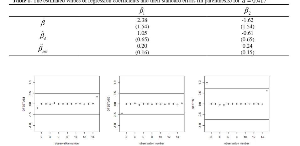
_srd), the standard errors are about 0.1, which shows that lower standard errors of the estimated parameters are achieved. Also as mentioned in [8], these additional information corrects the wrong sign problem of the estimated coefficients.

For more investigation, the DFBETAS values for the

jth (

j

=

1, 2

) element of

β



_srd and the

DFFITS

values are calculated and the results are presented in Figure 1. The Straight lines are the cutoff points. The cutoff

points are chosen as

2

n

+

p

and ₂ p n

, which are 0.48

and 0.73, respectively, for this study. From Figure 1, one can find out that only the first observation is recognized as influential with respect to the

DFFITS

criteria since the calculated value exceeds the cutoff point 0.73.

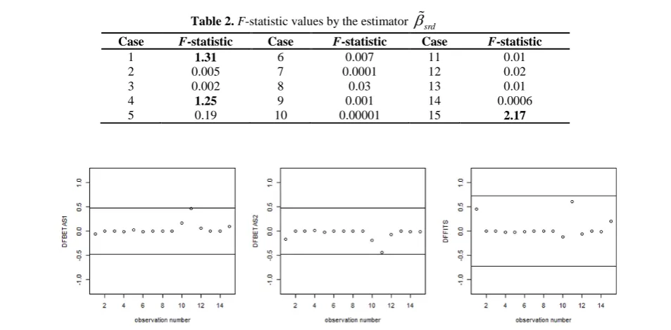
At last, we calculated the F-statistic in (40) for the fresh data. The results are given in Table 2. The first, the fourth and the fifteenth observations have the largest values of the F-statistic, which are 1.31, 1.25 and 2.17, respectively. For other observations, the F-statistic is obtained less than 1. Therefore, since

χ

₍₁₎2

=

3.84

(for

0.05

α

=

), none of the observations can be considered as an outlier for this data set.

To reveal the efficiency of our methods, a shift is

Table 1. The estimated values of regression coefficients and their standard errors (in parenthesis) for

d

=

0.417

1

β

β

₂

β



2.38 -1.62

(1.54) (1.54)

d

β



1.05 -0.61

(0.65) (0.65)

srd

β



0.20 0.24

(0.16) (0.15)

imposed on the dependent variable to investigate its impact on finding the outlier and on diagnosing influential observations. We have chosen a shift equal to 0.52 (which is about two standard deviation of y) and exerted on 11th _{observation. In fact, the chosen shift}

value is the largest possible value such that ensures us that the error terms of the rescaled shifted data are still of the form AR(1). For the new data set, the Liu biasing parameter is estimated as d=0.855, where

2

ˆ

0.018

σ

=

. The corresponding calculated DFBETAS and

DFFIT

values are displayed in Figure 2.

As it is seen in Figure 2, the absolute value of the

DFBETAS and DFFITS criteria for the 11th _observation

tends to be near the cutoff points but do not exceed the corresponding values 0.48 and 0.73. Also, the imposed shift on 11th _{observation has reduced the influence effect}

of the first observation on the estimated fitted values. Also, the values of F-statistic for the shifted data is given in Table 3. It can be seen from table 3, the calculated F-statistic for the 11th _{observation is 4.73 and}

for other observations, it is less than 3. So, since

2 (1)

7.70

>

χ

=

3.84

, the 11th _{observation is correctly}

recognized as an outlier.

Simulation study

In what follows a simulation study is carried out to investigate the performance of the proposed mean-shift outlier model and to conduct a survey on changes in influential measures in the presence of influential observation. Following McDonald and Galarneau [29], two collinear explanatory variables are generated from the following equation:

1 2 3

1

(

)

,

ij ij i

x

λ

z

z

λ

−

=

+

i

=

1,..., ,

t

j

=

1, 2

where

z

_i1,

z

_i2 and

z

_i3 are independent standard normal pseudo-random numbers, and

λ

represents the correlation between two explanatory variables

x

₁ and

Table 2. F-statisticvalues by the estimator

β



_srd

Case F-statistic Case F-statistic Case F-statistic

1 1.31 6 0.007 11 0.01

2 0.005 7 0.0001 12 0.02

3 0.002 8 0.03 13 0.01

4 1.25 9 0.001 14 0.0006

5 0.19 10 0.00001 15 2.17

Figure 2.

DFBETAS

for

β

₁ (

DFBETAS

₁) and DFBETAS for

β

₂ (

DFBETA S

₂) and

DFFITS

for fitted values by the estimator

β



_srd after changing the 11th _{observation. The straight lines are cutoff points.}

Table 3.F-statistic value by the estimator

β



_srd after changing the 11th _observation

Case F-statistic Case F-statistic Case F-statistic

1 0.65 6 0.003 11 4.73

2 0.0001 7 0.0004 12 2.59

3 0.00003 8 0.009 13 0.000004

4 0.36 9 0.002 14 0.003

2

x

, which is set to be 0.9 and 0.99 in this study. Also, the response variable is generated based on the model

2

1

i j ij i

j

y

β

x

ε

=

=

∑

+

,

i

=

1,...,

t

, with

ε

_i

=

ρε

_i−1

+

u

_i,

where

u

_i

~

NID

(0,1)

and the initial value

ε

₀ is sampled from

N

(0, (1

−

ρ

2

) )

−1 . The vector of coefficients is set to

β

=

(1, 0.5)

−

′

. With 0.6 and 0.9 values of

ρ

, 75, 90, 130 and 160 units of samples are produced for 1000 times. Each time the first 60 observations are taken as historical data, and after being rescaled by the unit length scaling technique, they are used for estimating the

ρ

parameter. The remaining (i.e.

n

=

15

, 30, 70 and 100) are taken as fresh data. Also for the fresh data, the

x

₁,

x

₂ and y values are rescaled. Furthermore, the 59th _{and 60}th _historical

data(which are the nearest observations to the fresh data) are used as the stochastic restrictions. In each iteration, the optimal

d

Liu parameter is found for the stochastic restricted Liu regression under AR(1). For different values of

λ

,

ρ

and

n

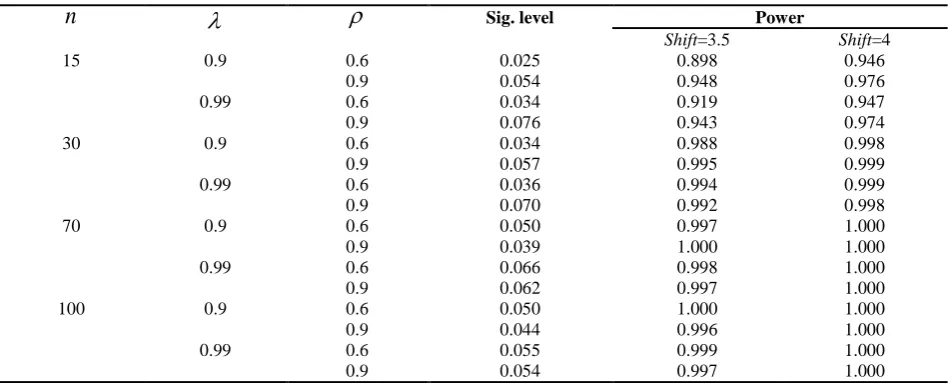
, the probability of type I error (

α

=

0.05

) is calculated using the method of mean-shift outlier model. For this purpose, the percentage of the time that the F-statistic for testing

0

:

0

H

γ

=

is greater than the corresponding critical value is calculated and the results are shown in Table 4. A glance in the results of this table indicates that the significance level remains around 0.05.

Also, the power of the test for the mean-shift outlier model is investigated in Table 4 after shifting the

generated data set. At this point, in each dataset, the 4th

fresh observation is taken as an outlier by exerting two shift values 3.5 and 4 to the original value of the response. These values are more than one time the mean of standard deviation of generated dependent observations and less than twice of it. Then the power of the test is calculated for the shifted data by the foregoing method. We remind that also here the shifted data are rescaled and before being used in the calculations, they’re AR(1) structure is checked by the Durbin-Watson statistic. It is shown in Table 4 that for each combination of

n

,

λ

and

ρ

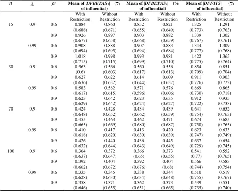
, the power of the test increases with the increase of the value of the shift. Also, it increases by the increase in the sample size.

In order to study the impact of the shifted 4th

observation on the estimated regression coefficients

β

₁,

2

β

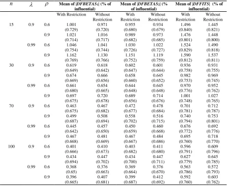
the predicted values of the response variable, the mean of absolute values of the

DFBETAS

and

DFFITS

in 1000 replications, with and without stochastic linear restrictions, are computed. The results are shown in Tables 5 and 6 for the shift values 3.5 and 4. The proportion of times that the absolute values of calculated

DFBETAS

and

DFFITS

values exceed

the cutoff points 2 n+p

and ₂ p n

(in which

p

=

2

in this study) are reported in parenthesis.

From Tables 5 and 6, it can be seen that for larger sample sizes, the mean of

DFBETAS

,

DFFITS

and their related proportions for the stochastic linear restrictions cases are smaller than the

Table 4. The probability of type I error and Power of the F test for the mean-shift outlier model for

( ,

β β

_{1 2}

) (1, 0.5)

= −

n

λ

ρ

Sig. level Power

Shift=3.5 Shift=4

15 0.9 0.6 0.025 0.898 0.946

0.9 0.054 0.948 0.976

0.99 0.6 0.034 0.919 0.947

0.9 0.076 0.943 0.974

30 0.9 0.6 0.034 0.988 0.998

0.9 0.057 0.995 0.999

0.99 0.6 0.036 0.994 0.999

0.9 0.070 0.992 0.998

70 0.9 0.6 0.050 0.997 1.000

0.9 0.039 1.000 1.000

0.99 0.6 0.066 0.998 1.000

0.9 0.062 0.997 1.000

100 0.9 0.6 0.050 1.000 1.000

0.9 0.044 0.996 1.000

0.99 0.6 0.055 0.999 1.000

measures for the cases with no stochastic linear restrictions. This result may be due to the achievement of improved accuracy for the advanced model when the sample size is enough large, and its reduced sensitivity to the observation which do not have a large displacement from the bulk of data.

For fix values of

λ

and

ρ

, the mean value of

DFBETAS

and

DFFITS

decreases as

n

increases for both models. But not any significant effect on the proportion of detection of influential observation can be shown. This may happen because cutoff points have an inverse relationship with the sample size and they decrease by the increase of

n

. So although we have a decrease in the mean of absolutes of measures, but simultaneously a decrease in cutoff points happens and causes the proportions to remain almost unchanged. It can also be seen from Tables 5 and 6 that with the

increase in the degree of collinearity (

λ

from 0.9 to 0.99), the mean value of the measures increases for small samples while it decreases for large samples. Also, it is seen in all cases that increasing of

ρ

(the autocorrelation parameter) causes a gr