Please cite this article in press asBanjoko A.W., Yahya W. B., Garba M. K.. Multiclass Response Feature Selection and Cancer Tumour Classification With Support Vector Machine. J Biostat Epidemiol. 2019; 5(2): 91-104
J Biostat Epidemiol. 2019;5(2): 91-104
Original Article
Multiclass Response Feature Selection and Cancer Tumour Classification With Support
Vector Machine
A. W. Banjoko, W. B. Yahya*, M. K. Garba
Department of Statistics, University of Ilorin, P.M.B. 1515, Ilorin, Nigeria.
ARTICLE INFO ABSTRACT
Received 18.09.2018 Revised 01.11.2018 Accepted 15.01.2019 Published 01.05.2019
Key words: Support Vector Machines; Monte-Carlo Cross-Validation; F-Statistic,
Family wise error rate, Misclassification Error Rate.
Background & Aim: In this study, efficient Support Vector Machine (SVM) algorithm for feature selection and classification of multi-category tumour classes of biological samples using gene expression profiles was proposed.
Methods: Feature selection interface of the algorithm employed the F-statistic of the ANOVA–like testing scheme at some chosen family-wise-error-rate which ensured efficient detection of false-positive genes. The selected gene subsets using the above method were further screened for optimality using the Misclassification Error Rates yielded by each of them and their combinations in a sequential selection manner. In a 10-fold cross-validation, the optimal values of the SVM parameters with appropriate kernel were determined for tissue sample classification using one-versus-all approach. The entire data matrix was randomly partitioned into 95% training set to train the SVM classifier and 5% test set to evaluate the predictive performance of the classifier over 1,000 Monte-Carlo cross-validation runs. Published microarray breast cancer dataset with five clinical endpoints was employed to validate the results from the simulation studies.
Results: Results from Monte-Carlo study showed excellent performance of the SVM classifier with higher prediction accuracy of the tissue samples based on the few gene biomarkers selected by the proposed feature selection method.
Conclusion: SVM could be considered as a classification of multi-category tumour classes of biological samples using gene expression profiles.
Introduction
Early detection and determination of the tumour types is very important in the management and treatment of various forms of cancer. Non-clinical prediction of cancer tumours using gene expression profiling has been reported to be a credible and efficient alternative technique to clinical methods in the past few years due to its numerous advantages [1, 12, 12]. However, diagnosis of cancer problems with binary endpoints, being the most common, has been given prominent attention in the literature[1,2,16]
*Corresponding Author: [email protected],
while few discussions only exist for multiclass cancer problems[3].
92 The relevance of a given gene subset 𝑥 as
stated in [4] and [18] was described under three categories; (i) A feature (gene) 𝑥 is said to be strongly relevant (and predictive of the response class) when the removal of 𝑥 alone from the data always reduces the prediction accuracy of the classifier, (ii) A feature 𝑥 is considered to be weakly relevant if it is not strongly relevant on its own but when joined with other gene subset 𝑆 it improves the prediction accuracy of the classifier, and lastly (iii) A feature 𝑥 is considered to be irrelevant if it is neither strongly nor weakly relevant. The main objective in feature selection exercise, therefore, is to arrive at a classification model that would contain as minimum as possible, the most relevant gene subsets that best predicts the response categories of the tissue sample and maximizes the prediction accuracy of the model [17, 20].
Several machine learning methods have been introduced in the literature. Some of these methods were only developed for classification (Partial Least Squares (PLS), Support Vector Machines (SVM), etc.) while some others combined feature selection with class prediction (Least Absolute Shrinkage and Selection Operator (LASSO) [16], k-Sequential Selection
(k-SS)[19] methods among others).
The SVM is one of the state–of–the–art methods considered to be very efficient among its counterparts in the field of statistical learning and pattern recognition. Its theoretical development and applications have been appeared in many works [1, 2, 5, 6], most especially for binary tumor classes.
In this study, a modified feature selection technique for high-dimensional genomic data is provided using the F-statistic of the ANOVA-like testing method at some chosen family-wise-error-rate (FWER). The efficiency of the features selected by this method is examined on SVM classifier using the average Misclassification Error Rates (MERs) and some other performance
indices based on simulated and published microarray breast cancer datasets.
Material and Methods
Data Description
Two types of data were employed in this study. The first is a simulated high-dimensional dataset with multi-class response class. The second dataset is a real-life gene expression high-dimensional breast cancer data set with five distinct sub-tumor groups.
Simulated Dataset
Multiclass response high-dimensional dataset with 𝑛 = 150 samples and 𝑝 = 1000 genes (n
<< p) was simulated from multivariate normal distribution following the procedures adopted in [2, 3]. The data have three response class 𝑦 with the class labels 𝑦 = 1, 2 and 3 if a given tissue sample belongs to response classes (groups) 1, 2 and 3 respectively.
The entire 𝑛 × 𝑝 data matrix was simulated such that 50 × 1000 data matrix was each simulated for the tissue samples in each of the response groups 1, 2 and 3 with 𝑛1= 50, 𝑛2= 50 and 𝑛3 = 50 tissue samples from groups 1, 2 and 3 respectively each with 1000 gene variables and 𝑛1+ 𝑛2+ 𝑛3= 𝑛. That is, on each tissue sample (observation), 1000 genes expression profiles were simulated.
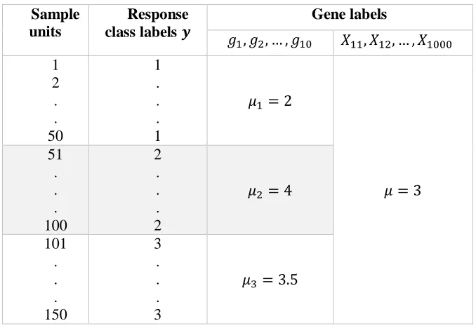
Out of the 1000 simulated gene expression profiles across the three response groups, 10 of them with gene labels 𝑔1, 𝑔2, … , 𝑔10 were simulated to be differentially expressed gene biomarkers and correlated with the response groups 𝑦. To achieve this, each of them was simulated from the mixture of three multivariate Gaussian densities with means µ1, µ2 and µ3 and variance-covariance matrices ∑1 , ∑2 and ∑3 respectively, µ1, µ2, µ3> 0 and µ𝑗 ≠ µ𝑗′, 𝑗, 𝑗′= {1,2,3} . That is, (𝑔1, 𝑔2, … , 𝑔10)|𝑦 ~ [𝜋1∗ 𝑁(µ1, ∑1) + 𝜋2∗ 𝑁(µ2, ∑2) + 𝜋3∗ 𝑁(µ3, ∑3)] with the mixing parameter 𝜋𝑗=
1
93 The remaining 990 genes with gene labels
𝑋11, 𝑋12, … , 𝑋1000 and possess relatively low
expression levels were simulated from
multivariate normal densities with means µ and variance-covariance matrix Σ. In all cases, the covariance matrix ∑ defined as ∑ = {𝜎𝑖𝑗}, has a block structure such that:
𝜎
𝑖𝑗= {
0.2,
𝑖𝑓|𝑗 − 𝑖| ≤ 5
0, 𝑜𝑡ℎ𝑒𝑟𝑤𝑖𝑠𝑒
An overview of the simulated microarray high dimensional data structure with multiclass responses is provided in Table 1.
Table 1: An overview of the simulated multiclass microarray data structure
Sample units
Response class labels 𝒚
Gene labels
𝑔1, 𝑔2, … , 𝑔10 𝑋11, 𝑋12, … , 𝑋1000
1 2 . . 50
1 . . . 1
𝜇1 = 2
𝜇 = 3 51
. . . 100
2 . . . 2
𝜇2 = 4
101 . . . 150
3 . . . 3
𝜇3= 3.5
Published Datasets
The real-life microarray cancer data used in this work is a published microarray breast cancer dataset than contained 456 gene expression profiles measured on 85 tissue samples with five distinct types of breast cancer tumours as the response classes [3, 9]. The five response classes are labeled A, B, C, D, E for ease of identification. The data can be accessed at
https://github.com/ramhiser/datamicroarray/
wiki/Sorlie-(2001)
Methodology
Feature Selections
By the high dimensional nature of the data employed with small sample units (n) and large number of features (p),𝑛 ≪ 𝑝, the identification
and selection of the few relevant gene biomarkers that are correlated with the tissue samples is very desirable. As a result, efficient method for extracting the informative features from the data was employed in this work given the nature of the data.
In both the simulated and real life datasets described above, the feature selection is performed using the F-statistic given by
𝐹 =
1
𝑘−1∑ 𝑤𝑗(𝑥̅𝑗−𝑥̅′)2 𝑘
𝐽=1
1+2(𝑘−2) 𝑘2−1∑ (
1 𝑛𝑗−1)(1−
𝑤𝑗 𝑤)
2 𝑘
𝐽=1
~𝐹𝑘−1,𝑣 (1)
where 𝑤𝑗= 𝑛𝑗
𝑆𝑗2 , 𝑤 = ∑ 𝑤𝑗 𝑘
𝑗=1 , 𝑥̅′ =
∑𝑘𝑗=1𝑤𝑗𝑥̅𝑗
𝑤
94
𝑣 = 𝑘2−1 3 ∑ ( 1
𝑛𝑗−1)(1− 𝑤𝑗
𝑤) 2 𝑘
𝑗=1
(2)
This feature selection process employed the F-statistic in the Analysis of Variance (ANOVA)-like testing method for comparing more than two treatment means at some chosen family-wise-error-rate (FWER), 𝛼𝐹. However, in order to control the number of false positive genes in the feature selection process, an adjusted Type I error level 𝛼 is used using the Sidak [11] method given by;
𝛼𝑠= 1 − (1 − 𝛼𝐹) 1⁄𝑝
(3)
where 𝑝 is the number of features in the microarray data. Thus, for any given FWER 𝛼𝐹, the value of Sidak 𝛼𝑠 in (3) is determined and used for feature selection. In this study, the six different 𝛼𝐹 values (in %) considered are 1%, 5%, 10%, 15%, 20% and 100%.
In its implementation, a particular feature
say
𝑋
𝑗will be regarded as a biomarker gene
feature if its p-value, say
𝑝
𝑗computed from
the F-statistic in (1) is less than
𝛼
𝑠(i.e. if
𝑝
𝑗< 𝛼
𝑠) [1].
SVM Implementation
The basic idea of the SVM as pointed out in [1] is to construct an optimal separating hyperplane for two-response groups gene expression data by mapping the data to a higher-dimensional space. This involves finding a hyperplane defined by a weight vector 𝒘 and a bias 𝒃 such that the separation of the two groups is maximized in a specific sense. Using kernel representations, linear separation in the higher-dimensional space corresponds to a nonlinear decision boundary in the original space. More details on this are provided in [1, 2, 5, 6] and the like.
In the case of 𝑘 classes response groups with 𝑘 > 2, the concept of separating hyperplane upon which the traditional SVM was developed does not lend itself naturally to a such number of groups [7,19]. Hence, the practice is to partition
the 𝑘 classes into several binary cases using either the one-versus-one or one-versus-all
approach [3] as adopted here. The idea is to fit 𝑘 SVMs and at each time comparing one of the 𝑘 classes to the remaining 𝑘 − 1 classes. The 𝑘𝑡ℎ response class will be coded as +1 while the remaining class groups will be coded as −1.
As a kernel-based machine learning method, the traditional SVM uses four types of kernel which include the Linear, Polynomial, Radial Basis Function (RBF) and Sigmoid kernels. The type of kernel employed plays a major role in the performance of the SVM method and this is largely dependent on the structure of the data being analyzed [1, 2, 5, 6]. As a result, the appropriate kernel type that is most efficient on the data being analyzed has to be determined before the classification task described above is performed.
For high-dimensional data when 𝑛 ≪ 𝑝, the linear kernel has been found to be suitable [1] and this shall be employed here for the case when all the gene features are to be used by the SVM classifier. On the other hand, when several gene subsets as determined by the feature selection results of the F-statistic at each of the chosen 𝛼𝐹 levels of 1%, 5%, 10%, 15%, 20%, and 100% are passed into the SVM algorithm for classification, the RBF kernel which has been reported to be more efficient on low dimensional data (the case of 𝑛 ≫ 𝑝) [1] shall be employed. Generally in this work, the optimal values of the SVM and kernel parameters for each dataset are determined through grid search in a 10-fold cross-validation for efficient SVM classification results.
95 Generally, the SVM classification method
described above is implemented on the gene subsets selected using the F-statistic at each of the six chosen 𝛼𝐹 values of 1%, 5%, 10%, 15%, 20% and 100% considered. The performance of the SVM classifier using each gene subset is then assessed by MER and other performance indices. As a further step to optimize the genes selected using the p-values of the F-statistic, all the genes present in the data are ranked in increasing order of their p-values contributions using a cluster of the first(best) 5, the first 10, the first 20 and the first 25 genes for SVM classification. The gene subset with the least MER of the SVM classifier is then observed. These observed genes were then reselected to optimize the feature selection phase for efficient SVM classification.
The proposed SVM algorithm was
implemented using e1071 package within the R environment (https://www.R-project.org/).
The proposed SVM algorithm explores the following steps:
Step 0: Start
Step 1: Determine the genes (features) that are differentially expressed from among the p
genes in the entire data using the F-statistic in equation (1) at a chosen 𝛼𝐹 level by testing the
hypothesis set:
𝐻0: 𝜇1= 𝜇2= ⋯ = 𝜇𝑘 (all the genes k
are not differentially expressed) 𝑣𝑠.
𝐻1: 𝑁𝑜𝑡 𝐻0 (gene g is differentially
expressed)
Step 2: Fit the SVM classifier on each of the gene subsets generated in step 1 and determine the values of SVM and kernel’s parameters for further use.
Step 3: Rank the genes in the gene subset obtain in step 3 by their respective p-values
Step 4: Fit the SVM classifier on each of the gene subsets obtained by the p-values ranks and select the subset with minimum average Misclassification Error Rate (MER).
Step 5: End
The proposed algorithm above is similar to the one proposed in [1] with a slight modification in
the feature selection method to accommodate multiclass responses as presented in [10].
Data Analysis
The analysis of the simulated and real-life datasets following the proposed SVM algorithm is presented in this section.
In the analysis of each dataset, the data were randomly partitioned into a 95% training test and 5% test set. By this, full information on the 95% of the sampled data was used to train the SVM
algorithm with the performance of the
classification model so constructed were assessed on the remaining left-out 5% test sample data over 1000 Monte-Carlo Cross-validation runs. As a first step, the feature selection was performed on the two data sets using the F-statistic as presented in (1) through (3). Here, the strength of association between individual gene variable and the multi-category response class is determined by the p-values that are associated with their respective F-statistic values. For instance, if all the 1000 genes in the simulated dataset are ranked by their respective p-values (computed from their F-statistic values) in ascending order of magnitude, the gene variable having the least p-value is adjudged to be the most strongly related to the response class followed by the next and so on.
The strength of the relationship of each of the gene variables with the response classes in each dataset was determined by their respective p-values with which all the genes were ranked accordingly. The ranked genes were selected based on the computed thresholds of Sidak 𝛼𝑠 values in (3) as determined by the FWER 𝛼𝐹. Thus, for a given 𝛼𝐹, the gene subsets whose p-values are not more than the computed Sidak alpha value 𝛼̂𝑠 were selected from among the ranked genes as the differentially expressed genes and these were passed into SVM algorithm for classification.
96 alternative method adopted for gene selection
here is to selected the first k genes among the ranked genes where k = 5, 10, 15, 20 and 25. Thus, the first 5, first10, first15, first 20 and first 25 genes were selected from the ranked genes for SVM implementations. By this, it is possible to determine the marginal contribution brought into the performance of the SVM algorithm by the additional gene variables added at each gene selection.
More generally, at each SVM implementation, the SVM’s and kernel’s parameters were efficiently determined for each data set over 10-fold cross-validation.
Results
The results of the proposed SVM algorithm for feature selection and classification of tumor samples with multiclass responses for both the simulated and published breast cancer dataset are presented in this section.
Results for Simulated Data
The analysis started by performing features selection on all the 1000 simulated genes using the F-statistic in (1). The set of differentially expressed genes selected at the chosen different FWER as used in the computation of Sidak alpha in (3) are presented in Table 2.
Table 2: The number of differentially expressed genes (Biomarkers) selected using the F-Statistic at different FWER 𝛼𝐹 for simulated multiclass data .
𝜶𝑭 No. of
genes selected
Genes Selected
1% 9 𝑔6, 𝑔10, 𝑔2, 𝑔3, 𝑔1, 𝑔5, 𝑔9, 𝑔8, 𝑔7
5% 10 𝑔6, 𝑔10, 𝑔2, 𝑔3, 𝑔1, 𝑔5, 𝑔9, 𝑔8, 𝑔7, 𝑔4
10% 10 𝑔6, 𝑔10, 𝑔2, 𝑔3, 𝑔1, 𝑔5, 𝑔9, 𝑔8, 𝑔7, 𝑔4
15% 11 𝑔6, 𝑔10, 𝑔2, 𝑔3, 𝑔1, 𝑔5, 𝑔9, 𝑔8, 𝑔7, 𝑔4, 𝑋284
20% 11 𝑔6, 𝑔10, 𝑔2, 𝑔3, 𝑔1, 𝑔5, 𝑔9, 𝑔8, 𝑔7, 𝑔4, 𝑋284
100% 1000 All the 1000 genes
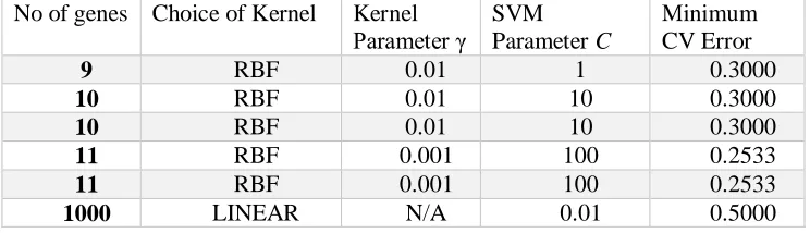
The set of the selected genes at each chosen FWER was used to train SVM classifier and determine the optimal values of the RBF kernel’s parameter (for low dimensional data space), the Linear kernel’s parameter (for high-dimensional
space) and the SVM parameter the results of which are presented in Table 3. In a 10-fold cross-validation runs, the minimum cross-cross-validation error of the SVM classifier at each optimal parameter pair is equally reported in Table 3.
Table3: Result s of the optimal tuning parameter values of SVM classifier with the Simulated Multiclass microarray data.
No of genes Choice of Kernel Kernel
Parameter γ SVM Parameter C
Minimum CV Error
9 RBF 0.01 1 0.3000
10 RBF 0.01 10 0.3000
10 RBF 0.01 10 0.3000
11 RBF 0.001 100 0.2533
11 RBF 0.001 100 0.2533
97 The optimal kernel and SVM parameters
determined as reported in Table 3 were used to train SVM classifier on each of the selected gene subsets the performance of which were examined using the test samples over 1000 MCCV runs.
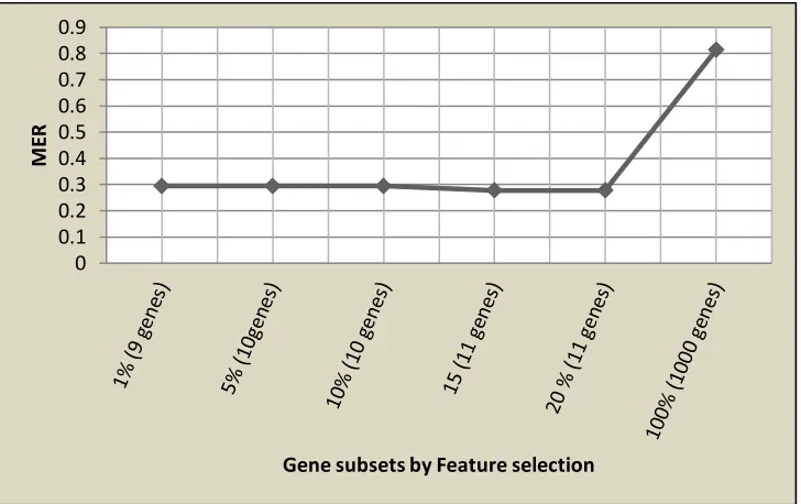
The classification results as provided by various performance indices are presented by Table 4. The plot of the average MER yielded by SVM algorithm over different gene subsets selected at various FWERs is presented by Fig 1.
Figure 1: Graph of MERs yielded by SWM algorithm at different selected gene subsets by p -value rank with FWERs thresholds .
Table 4: Result of the SVM classifier on each selected gene subsets at varying qqFWERs from the simulated data. The number of genes at which the best classification accuracy was achieved by the classifier is asterisked (*).
Performance Measure FWER (𝜶𝑭)
1% 5% 10% 15% 20% 100%
No of genes 9 10 10 11* 11 1000
MER 0.2947 0.2949 0.2949 0.2774 0.2774 0.8145
CCR (%) 70.530 70.510 70.510 72.260 72.260 18.550
Sensitivity A 0.6218 0.6286 0.6286 0.6349 0.6349 0.3259
Sensitivity B 0.6550 0.6471 0.6471 0.6732 0.6732 0.3477
Sensitivity C 0.8965 0.8765 0.8765 0.8955 0.8955 0.3264
Specificity A 0.7890 0.7591 0.7591 0.7906 0.7906 0.6495
Specificity B 0.8593 0.8548 0.8548 0.8516 0.8516 0.6731
Specificity C 0.9272 0.9538 0.9538 0.9526 0.9526 0.6980
Positive Predicted Value A 0.6001 0.5702 0.5702 0.6102 0.6102 0.1766
Positive Predicted Value B 0.7196 0.7155 0.7155 0.7126 0.7126 0.2261
Positive Predicted Value C 0.8741 0.9176 0.9176 0.9178 0.9178 0.2425 0
0.1 0.2 0.3 0.4 0.5 0.6 0.7 0.8 0.9
M
ER
98
Negative Predicted Value A 0.8036 0.8030 0.8030 0.8113 0.8113 0.6036
Negative Predicted Value B 0.8124 0.8122 0.8122 0.8240 0.8240 0.6289
Negative Predicted Value C 0.9630 0.9573 0.9573 0.9640 0.9640 0.6221
Results from Table 4 showed that the SVM classifier provided the best classification results using only 11 gene subsets selected at 𝛼𝐹 = 15%. At this gene subset, the classification accuracy (CCR) of the SVM classifier was about 72% with appreciable results reported on all other
performance indices. It is quite interesting to note that the performance of the SVM classifier was worst with about 18% classification accuracy when 1000 gene expression profiles selected at 𝛼𝐹 = 100% were employed for classification.
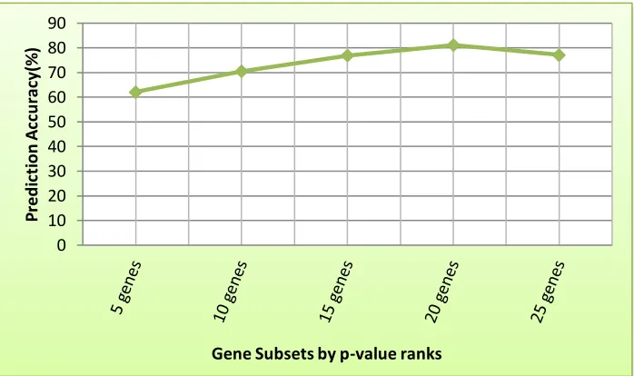
Figure 2: Graph of MERs yielded by SWM algorithm at different selected gene subsets up to the first 25 genes by p-value rank.
Table 5 presented the results of the kernel and SVM parameters using the first 5, first 10, first 15, first 20 and first 25 genes among the ranked
genes selected by the p-values of the F-statistic values. The results of the SVM classifiers based on these selected genes are presented in Table 6.
Table 5: Result s of RBF and SVM tuning parameter for each of the ranked gene subsets for the simulated data.
No. of genes Selected by p-value ranks
Kernel Parameter 𝜸
SVM Parameter 𝑪
Minimum CV Error
5 0.05 1 0.3533
10 0.01 10 0.3000
15 0.01 1 0.2533
20 0.00001 10000 0.2000
25 0.1 1 0.1933
0 10 20 30 40 50 60 70 80 90
P
red
ic
ti
o
n
A
cc
u
ra
cy(%
)
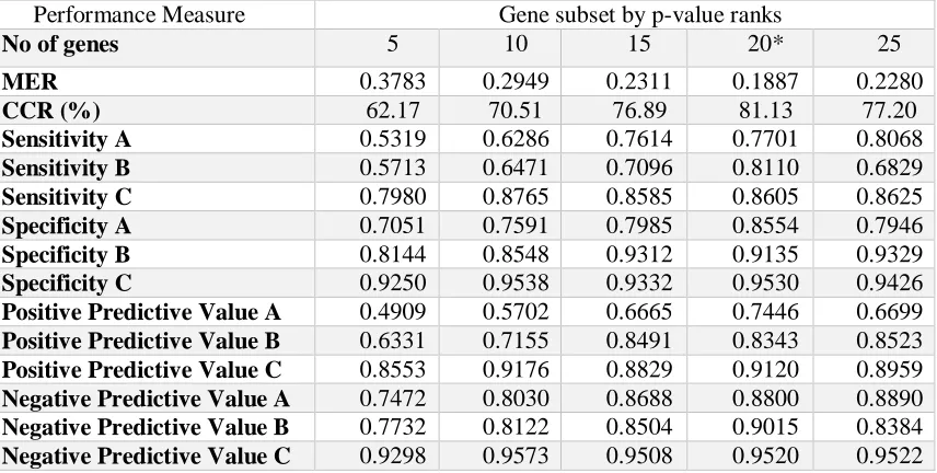
99 Table 6: Result of the SVM classifier on each selec ted gene subsets up to the first 25 genes selected by p-value rank from the simulated data. The number of genes at which the best classification accuracy was achieved by the classifier is asterisked (*).
Performance Measure Gene subset by p-value ranks
No of genes 5 10 15 20* 25
MER 0.3783 0.2949 0.2311 0.1887 0.2280
CCR (%) 62.17 70.51 76.89 81.13 77.20
Sensitivity A 0.5319 0.6286 0.7614 0.7701 0.8068
Sensitivity B 0.5713 0.6471 0.7096 0.8110 0.6829
Sensitivity C 0.7980 0.8765 0.8585 0.8605 0.8625
Specificity A 0.7051 0.7591 0.7985 0.8554 0.7946
Specificity B 0.8144 0.8548 0.9312 0.9135 0.9329
Specificity C 0.9250 0.9538 0.9332 0.9530 0.9426
Positive Predictive Value A 0.4909 0.5702 0.6665 0.7446 0.6699
Positive Predictive Value B 0.6331 0.7155 0.8491 0.8343 0.8523
Positive Predictive Value C 0.8553 0.9176 0.8829 0.9120 0.8959
Negative Predictive Value A 0.7472 0.8030 0.8688 0.8800 0.8890
Negative Predictive Value B 0.7732 0.8122 0.8504 0.9015 0.8384
Negative Predictive Value C 0.9298 0.9573 0.9508 0.9520 0.9522
Results for Published Data
The same procedures adopted to analyze the simulated dataset and obtain the various results as
reported in Tables 2 to 6 were also adopted to implement the SVM classifier on the real-life cancer data set.
Table 7: Result of the optimal tuning parameter values of SVM classifier selected gene subsets from the Breast Cancer data.
𝜶𝑭 level in %
(No of genes selected)
Choice of
Kernel
SVM
Parameter C
Minimum CV error
1% (90) Linear 0.01 0.0681
5% (131) Linear 0.01 0.0792
10% (138) Linear 0.01 0.0792
15% (155) Linear 0.01 0.0681
20% (165) Linear 0.01 0.0792
100% (456) Linear 0.01 0.1042
Feature selection with different FWERs was performed to obtain varying subsets of gene combinations using the F-statistic. These were used by the SVM algorithm to determine the
100 each of the chosen FWER is more than the
number of tissue samples, n in the data, the linear kernel, which is most appropriate in this case, was employed in the implementation of SVM algorithm as shown in Table 7.
The classification results of the SVM algorithm based on the various gene subsets
selected at different FWERs are presented in Table 8. Also, the results of the SVM classifier using the first 25 selected genes ranked by their p-values as computed from the values of their F-statistics are presented in Table 9.
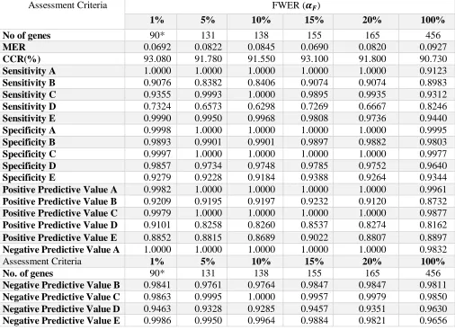
Table 8: Result of the SVM method on each selected gene subsets at varying FWERs from the Breast cancer data. The number of genes at which the best classification accuracy was achieved by the classifier is asterisked (*).
Assessment Criteria FWER (𝜶𝑭)
1% 5% 10% 15% 20% 100%
No of genes 90* 131 138 155 165 456
MER 0.0692 0.0822 0.0845 0.0690 0.0820 0.0927
CCR(%) 93.080 91.780 91.550 93.100 91.800 90.730
Sensitivity A 1.0000 1.0000 1.0000 1.0000 1.0000 0.9123
Sensitivity B 0.9076 0.8382 0.8406 0.9074 0.9074 0.8983
Sensitivity C 0.9355 0.9993 1.0000 0.9895 0.9935 0.9312
Sensitivity D 0.7324 0.6573 0.6298 0.7269 0.6667 0.8246
Sensitivity E 0.9990 0.9950 0.9968 0.9808 0.9736 0.9440
Specificity A 0.9998 1.0000 1.0000 1.0000 1.0000 0.9995
Specificity B 0.9893 0.9901 0.9901 0.9897 0.9882 0.9803
Specificity C 0.9997 1.0000 1.0000 1.0000 1.0000 0.9977
Specificity D 0.9857 0.9734 0.9748 0.9785 0.9752 0.9640
Specificity E 0.9279 0.9228 0.9184 0.9388 0.9264 0.9344
Positive Predictive Value A 0.9982 1.0000 1.0000 1.0000 1.0000 0.9961
Positive Predictive Value B 0.9209 0.9195 0.9197 0.9232 0.9120 0.8732
Positive Predictive Value C 0.9979 1.0000 1.0000 1.0000 1.0000 0.9877
Positive Predictive Value D 0.9101 0.8258 0.8260 0.8537 0.8274 0.8162
Positive Predictive Value E 0.8852 0.8815 0.8689 0.9022 0.8807 0.8897
Negative Predictive Value A 1.0000 1.0000 1.0000 1.0000 1.0000 0.9832
Assessment Criteria 1% 5% 10% 15% 20% 100%
No. of genes 90* 131 138 155 165 456
Negative Predictive Value B 0.9841 0.9761 0.9764 0.9847 0.9847 0.9811
Negative Predictive Value C 0.9863 0.9995 1.0000 0.9957 0.9979 0.9850
Negative Predictive Value D 0.9463 0.9328 0.9285 0.9457 0.9351 0.9630
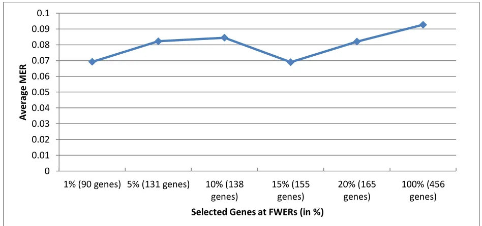
101 Figure 3: Graph of Misclassification Error Rate (MER) of SVM method for the Breast cancer data at different FWERs (in %). The numbers of genes selected are in parenthesis.
Table 9: Classification r esult s of SVM method on each selected ranked gene subsets from the Breast Cancer data.
Performance Measure Gene subset by p-value ranks
No of genes 5 10 15 20 25*
MER 0.2870 0.2010 0.1565 0.1675 0.1145
CCR(%) 71.300 79.900 84.350 83.250 88.550
Sensitivity A 0.9982 1.0000 1.0000 0.9994 0.9994
Sensitivity B 0.6454 0.7490 0.6762 0.7611 0.7579
Sensitivity C 0.6206 0.9049 0.8686 0.9824 0.9863
Sensitivity D 0.3456 0.3770 0.6728 0.5861 0.7126
Sensitivity E 0.8209 0.8678 0.9004 0.8159 0.9055
Specificity A 0.9875 0.9988 0.9885 0.9882 0.9875
Specificity B 0.9878 0.9875 0.9640 0.9584 0.9770
Specificity C 0.9590 0.9619 0.9726 1.0000 0.9992
Specificity D 0.8395 0.9019 0.9309 0.8932 0.9377
Specificity E 0.8539 0.8821 0.9464 0.9518 0.9499
Positive Predicted Value A 0.9445 0.9946 0.9514 0.9505 0.9487
Positive Predicted Value B 0.8863 0.8939 0.7219 0.7095 0.8294
Positive Predicted Value C 0.7405 0.8240 0.8658 1.0000 0.9951
Positive Predicted Value D 0.2940 0.4279 0.6603 0.5150 0.6836
Positive Predicted Value E 0.7731 0.8137 0.9091 0.9060 0.9231
Performance Measure Gene subset by p-value ranks
No of genes 5 10 15 20 25*
Negative Predicted Value A 0.9993 1.0000 1.0000 0.9995 0.9995
Negative Predicted Value B 0.9488 0.9625 0.9523 0.9638 0.9631
Negative Predicted Value C 0.9278 0.9816 0.9726 0.9965 0.9974
Negative Predicted Value D 0.8670 0.8808 0.9323 0.9183 0.9454
Negative Predicted Value E 0.8934 0.9192 0.9462 0.9035 0.9462 0
0.01 0.02 0.03 0.04 0.05 0.06 0.07 0.08 0.09 0.1
1% (90 genes) 5% (131 genes) 10% (138 genes)
15% (155 genes)
20% (165 genes)
100% (456 genes)
A
ve
ra
ge
M
ER
102
Discussion of Results
This work presents an efficient algorithm for implementing Support Vector Machine method for feature selection and classification of biological samples in multiclass response cancer tumor problems. The proposed feature selection technique in this study was able to detect and selected all the differentially expressed genes at a very low 1% FWER in Monte-Carlo study as presented in Table 2. Although, very few other genes were also detected as differentially expressed and this may be due to the value of the parameters specified in the simulation study.
The SVM algorithm as implemented in this work yielded good prediction accuracies (low misclassification error rates) with few selected biomarker genes than when all the available gene variables were used for classification of the response classes. This is an indication that the presence of noisy (irrelevant) genes in the set of features employed may adversely affect the performance of a good classifier.
The determination of the optimal values of the kernel and SVM parameters that are desirable and suitable for a given data structure play important roles in improving the performances of the SVM classifier. This is evident by the results of cross-validation error rates reported by the SVM at the optimal values of the kernel and SVM parameters as reported in Tables 3, 5 and 7 for the two data sets analyzed here.
Considering the performance of the SVM classifier at the chosen different FWERs, classification results reported in Table 4 showed that the classifier yielded the best prediction accuracy (PA) at 15% FWER at which only 11 gene subsets were selected and employed by SVM method for classification of the response class in the simulated data. The PA yielded by SVM classifier with these 11 gene biomarkers is about 72%. It can be observed that more genes selected at higher values of FWER especially when all the genes variables were employed (at 𝛼𝐹 = 100%) clearly worsened the performance of
the SVM classifier with the poorest PA of about 18%!
Results from Table 6 showed improved performance of the SVM algorithm as the number of gene subsets used increases among the ranked genes beginning from the first 5 genes up to the first 20 genes on the rank after which the prediction accuracy (PA) of the SVM decreases for simulated data (i.e. first 5 (PA= 62.17%); first 10 (PA = 70.51%); first 15(PA = 76.89%); first 20 (PA = 81.13%); first 25(PA = 77.2%)). The results of other performance indices like the sensitivity, specificity, positive and negative predictive values followed this same trend as can be observed from the classification results in Table 6. These results, therefore, showed that inclusion of additional five gene variables from 20 to 25 genes into the SVM algorithm failed to improve the efficiency of the classifier since its performance becomes worst off using more than 20 gene variables.
103 9. The result of the SVM classifier on each of the
ranked subsets also follows the pattern observed in the simulated data result. An appreciable increase in the accuracy (i.e. first 5 – 71.3%, first 10 – 79.9%, first 15 – 84.35%, first 20 – 83.25%, and first 25 – 88.55%) of the algorithm from each ranked subsets was noticed with a slight fall in the accuracy when the number of genes is twenty-five. This indicated that some noisy (false positive) genes were present in the gene combination at the ranked subset of the first twenty genes.
Conclusion
An efficient algorithm for feature selection and classification of tissue samples with support vector machine in high-dimensional microarray multiclass responses is presented in the study.
As common in many feature selection and classification studies with microarray cancer data where the data will possess greater number of genes variables that are purely uncorrelated with the clinical outcomes of the tissue samples, the new proposed method in this study yielded appreciable improvement in its ability to identify and select few gene biomarkers that seems to be biologically related to the response classes of the tissues samples. This has tremendously improved the performance of the SVM classifier that employed the few selected differentially genes for class prediction in out-of samples situations than when the entire available genes in the data were used. This result shows that the proposed method is more parsimonious at optimizing feature selection for good response class prediction than the traditional SVM method.
References
1. Banjoko A.W., Yahya W. B., Garba M. K., Olaniran O. R., Olorede K. O., Dauda K. A., Efficient Support Vector Machine Classification of Diffuse large B-Cell Lymphoma and Follicular Lymphoma mRNA Tissue Samples, Annals. Computer Science Series, 13, 2015a, 69 – 79.
2. Yahya W. B., Genes selection and Tumour Classification in Cancer Research: A new
approach, Säbruck, Germany: Lambert
Academic Publishing, 2012.
3. Yahya W. B., Aremu G. T., Garba M. K., Multiclass Sequential Feature Selection and Classification Method for Gene Expression Data, Journal of Applied Science and Technology, 20 (1&2), 2015, 50 – 61.
4. Witold R. R., Rudnicki, Mariusz W., Wiesław P., All Relevant Feature Selection Methods and
Applications, Studies in Computational
Intelligence, Springer, 584, 2015, 11 – 28. 5. Vapnik V. N., The Nature of Statistical Learning Theory, Springer-Verlag, New York, 1995.
6. Cristianini N., Shawe-Taylor J., An introduction to Support Vector Machines, Cambridge University Press, United Kingdom, 2012.
7. James G., Witten D., Hastie T., Tibshirani R., An Introduction to Statistical Learning with Applications in R, Springer Science + Business Media, New York, 2013.
8. Cichosz P., Data mining algorithms explained using R, John Wiley & Sons, New York., 2015. 9. Sørlie T., Perou C. M., Tibshirani R., Aas T., Geisler S., Johnsen H., Hastie T., Eisenh M. B., van de Rijn M., Jeffrey S. S., Thorsen T., Quist H., Matese J. C., Brown P. O., Botstein D., Lønning P. E., Anne-LiseBørresen-Dale, Gene expression patterns of breast carcinomas distinguish tumor subclasses with clinical implications”, Proceeding of the National Academy of Sciences of the United State of America (PNAS), 98, 2001, 10869 – 10874.
10. Welch B. L., On the comparison of
several
mean
values:
An
alternative
approach. Biometrika, 1951, 38
,
330–336.
11. Sidak Z. K., Rectangular Confidence Regionsfor the Means of Multivariate Normal
104 12. Banjoko A.W., Yahya W. B., Garba M. K.,
Efficient Support Vector Machine Method for Tissue Samples Classification in Colon Cancer Genomic data, Proceedings of the 34th Annual Conference of The Nigeria Mathematical Society, Nigeria, 2015b.
13. Banjoko A.W., Yahya W. B., Garba M. K., Support Vector Machine for Feature Selection and Classification of Small Node–Negative Breast Carcinomas, Proceeding of the 3rd International Conference of the U6 Consortium, Nigeria, 2015c.
14. Banjoko A.W., Yahya W. B., Garba M. K., Efficient Support Vector Machine Classification of Diffuse Large B-Cell Lymphoma and Follicular Lymphoma mRNA Tissue Samples, Proceedings of the14th Regional Scientific Conference of the International Biometric Society – group Nigeria, Nigeria, 2015d.
15. Hapfelmeier A., Yahya W. B., Rosenberg R., Ulm K., Predictive Modeling of gene Expression data. In: Handbook of Statistics in Clinical Oncology, Chapman and Hall/CRC,New York, 2012, 463-475.
16. Yahya W. B., Sequential dimension reduction and prediction methods with high dimensional
microarray data, Ph.D. Thesis, Ludwig
Maximilians-Universität, München, Germany, 2009.
17. Yahya W. B., Oladiipo M. O., Jolayemi E. T., A fast algorithm to construct neural networks classification models with high-dimensional genomic data, Annals. Computer Science Series, 10, 2012, 39- 58.
18. Yahya W. B., Rosenberg R., Ulm K.,
Microarray-based Classification of
Histopathologic Responses of Locally Advanced Rectal Carcinomas To Neoadjuvant Radio-chemotherapy Treatment, Turkiye Klinikleri Journal of Biostatistics, 6(1), 2014, 8- 23.
19. Yahya W. B., Ulm K., Ludwig F., Hapflemeir A., k-SS: A sequential feature selection and
prediction method in microarray study,
International Journal of Artificial Intelligence, 6, (S11), 2011, 19- 47.