Universal Approximation Results for the Temporal
Restricted Boltzmann Machine and the Recurrent Temporal
Restricted Boltzmann Machine
Simon Odense [email protected]
Roderick Edwards [email protected]
Department of Mathematics University of Victoria
Victoria, BC, 3800 Finnerty Rd, Canada
Editor:Yoshua Bengio
Abstract
The Restricted Boltzmann Machine (RBM) has proved to be a powerful tool in machine learning, both on its own and as the building block for Deep Belief Networks (multi-layer generative graphical models). The RBM and Deep Belief Network have been shown to be universal approximators for probability distributions on binary vectors. In this paper we prove several similar universal approximation results for two variations of the Restricted Boltzmann Machine with time dependence, the Temporal Restricted Boltzmann Machine (TRBM) and the Recurrent Temporal Restricted Boltzmann Machine (RTRBM). We show that the TRBM is a universal approximator for Markov chains and generalize the theorem to sequences with longer time dependence. We then prove that the RTRBM is a universal approximator for stochastic processes with finite time dependence. We conclude with a discussion on efficiency and how the constructions developed could explain some previous experimental results.
Keywords: TRBM, RTRBM, machine learning, universal approximation
1. Introduction
Bengio, 2008). Furthermore the related Deep Belief Networks have also been shown to be universal approximators even when each hidden layer is restricted to a relatively small number of hidden nodes (Sutskever and Hinton, 2010)(Le Roux and Bengio, 2010)(Montu-far and Ay, 2011). The universal approximation of CRBMs follows immediately from that of Boltzmann machines (Montufar et al., 2014). The question we wish to address here is the universal approximation of stochastic processes by TRBMs and RTRBMs.
1.1 The Restricted Boltzmann Machine
An RBM defines a probability distribution over a set of binary vectors x∈ {0,1}n=X as follows
P(v, h) = exp(v>W h+c>v+b>h)/Z
where the set of binary vectorsX is partitioned into visible and hidden units X =V ×H
and Z is the normalization factor, in other words Z =P v,h
exp(v>W h+c>v+b>h). This
distribution is entirely defined by (W, b, c) and is referred to as a Boltzmann Distribution. We are generally concerned with the marginal distribution of the visible units. When we refer to the distribution of an RBM we are referring to the marginal distribution of its visible units. The marginal distribution of a single visible node is given by
P(vi = 1|h) =σ
X j
wi,jhj+ci
where σ(x) = 1+exp(1 −x). A similar equation holds for the hidden units. Variations of the RBM which use real-valued visible and hidden units (or mixes of the two) exist but will not be considered here.
1.2 Approximation
In order to measure how well one distribution approximates another we use the Kullback-Leibler divergence, which for discrete probability distributions is given by
KL(R||P) =X
v
R(v) log
R(v)
P(v)
,
wherevranges over the sample space ofR andP. It can be shown that for any >0, given a probability distribution R on V there is a Boltzmann Distribution given by an RBMP
2. Universal Approximation Results for the TRBM
A TRBM defines a probability distribution on a sequence xT = (x(0), ..., x(T−1)), x(i) ∈
{0,1}n,x(i)= (v(i), h(i)), given by
P(v(t), h(t)|h(t−1)) = exp(v
(t)>W h(t)+c>v(t)+b>h(t)+h(t)>W0h(t−1))
Z(h(t−1)) ,
P(vT, hT) = T−1
Y k=1
P(v(k), h(k)|h(k−1)) !
P0(v(0), h(0)).
This distribution is defined by the same parameters as the RBM along with the additional parametersW0. The TRBM can be seen as an RBM with a dynamic hidden bias determined by W0h(t−1). The initial distribution, P
0(v(0), h(0)), is the same as P(v(t), h(t)|h(t−1)) with
h(0)>binit replacing h(t)>W0h(t−1) for some initial hidden bias binit. Note that W0 is not symmetric in general. We call the connections between h(t−1) and h(t) with weights inW0
temporal connections.
2.1 Universal Approximation Results for the Basic TRBM
Our approximation results will deal with distributions which are time-homogeneous and have finite time dependence. These distributions can be written in the form
R(vT) = T−1
Y k=m
R1(v(k)|v(k−1), ..., v(k−m)) !
R0(v(0), ..., v(m−1))
whereR1 is the transition probability andR0 is the initial distribution. We first show that a TRBM can approximate a Markov chain (distributions of the above form with m = 1) for a finite number of time steps to arbitrary precision. We begin by proving a lemma. HerePtis the marginal distribution ofP over (v(0), . . . , v(t)). SimilarlyR0,t is the marginal distribution of R0 over (v(0), . . . , v(t)).
Lemma 1: LetR be a distribution on a finite sequence of lengthT of n-dimensional binary vectors that is time homogeneous with finite time dependence. Given a set of distributions
P on the same sequences, if for every >0 we can find a distribution P ∈P such that for every vT,
KL(R1(·|v(t−1), ..., v(t−m))||P
t(·|v(t−1), ..., v(0)))< for m≤t < T −1,
KL(R0,t(·|v(t−1), ..., v(0))||Pt(·|v(t−1), ..., v(0)))< for 0< t < m,
and KL(R0,0(·)||P0(·))< ,
then we can find distributions P ∈P to approximate R to arbitrary precision.
Proof: The proof is given in the appendix.
Now we use this lemma to prove our first universal approximation theorem. In this caseP
Theorem 1: Let R be a distribution over a sequence of length T of binary vectors of length n that is time homogeneous and satisfies the Markov property. For any >0 there exists a TRBM defined on sequences of length T of binary vectors of length n with distri-bution P such thatKL(R||P)< .
Proof: By the previous lemma we will be looking for a TRBM that can approximate the transition probabilities of R along with its initial distribution. The proof will rely on the universal approximation properties of RBMs. The idea is that given one of the 2n con-figurations of the visible units, v, there is an RBM with distribution Pv approximating
R1(·|v(t−1) =v) to a certain precision. The universal approximation results for RBMs tell us that this approximation can be made arbitrarily precise for an RBM with enough hidden units. Furthermore, this approximation can be done with visible biases set to 0 (Le Roux and Bengio, 2008). We thus set all visible biases of our TRBM to 0 and include each of the approximating RBMs without difficulty. We label these RBMs H1, ..., H2n. Given a
specific configuration of the visible nodes v, Hv refers to the RBM chosen to approximate
R1(·|v(t−1)=v).
The challenge then is to signal the TRBM which of the 2n RBMs should be active at the next time step. To do this we include 2nadditional hidden nodes which we will call control nodes, each corresponding to a particular configuration of the visible units. Thus we add 2n control nodes,hc,1, ..., hc,2n corresponding to the hidden nodesH1, ..., H2n. Again, given
a particular visible configurationv, we denote the corresponding control node byhc,v. The set of all control nodes will be denotedHc. Note that (c, v) is the label ofhc,v and weights involvinghc,v will be denoted w(c,v),i orw0j,(c,v). The control nodes will signal which of the
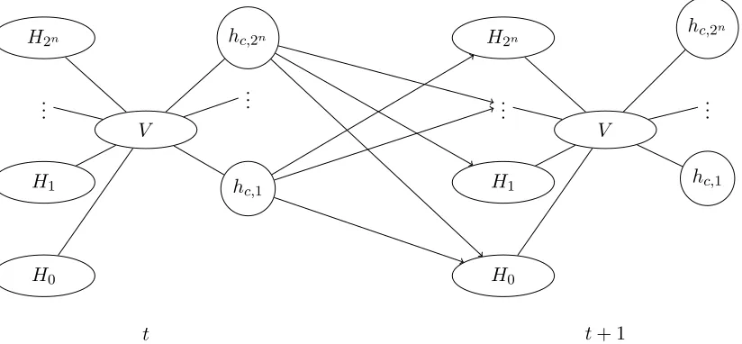
Hi’s should be active at the next time step. To accomplish this we will choose parameters such that whenv is observed at timet−1, hc,v will be on at timet−1 with a probability close to 1 and every other control node will be off at time t−1 with probability close to 1. Each hc,v will have strong negative temporal connections to every Hv0 with v0 6= v, in essence turning off every RBM corresponding to R1(·|v(t−1) = v0), and leaving the RBM corresponding to R1(·|v(t−1) = v) active (see Fig. 1). We will break the proof down into four parts and we must be able to choose parameters that satisfy all four conditions.
First, we must be able to choose parameters so that given v(t−1) = v, the probability thath(c,vt−1) = 1 can be made arbitrarily close to 1 and the probability thath(t
−1)
c,v0 = 1 can be made arbitrarily close to 0. Second, we must have that the control nodes have no impact on the visible distribution at the same time step so the transition probabilities of the TRBM will still approximate R1(·|v(t−1) = v). Third, we must be able to choose parameters so that givenh(c,vt−1) = 1 andhc,v(t−01)= 0, the probability that any nodes inHv0 are on at timet can be made arbitrarily close to 0 for v0 6=v. Finally, we must be able to approximate the initial distributionR0.
encode the visible state in the control unit so that information can be passed to the hidden nodes at the next time step without the encoding changing the visible distribution. This is covered in Steps 1 and 2. Step 3 verifies that the correct distribution can be recovered from the encoding and Step 4 shows we can simulate the initial distribution without changing the rest of the machine.
hc,2n
hc,1
H2n
H1
H0
V
..
. ...
hc,2n
hc,1
H2n
H1
H0
V
..
. ...
t t+ 1
Figure 1: Interactions between sets of nodes within and between time steps: eachhc,v turns off everyHv0 :v6=v0 in the subsequent time step. hc,v will only be
on ifv is observed at timetand collectively the control nodesHc have negligible
effect on the visible distribution. H0 is an additional set of hidden units that
will be used to model the initial distribution.
To choose temporal connections, define w0j,(c,v) to be −α if hj ∈ Hv0 where v0 6= v and 0 otherwise. Let every otherw0i,j = 0. In particular, remembering that W0 is not necessarily symmetric, we have w0(c,v),j = 0 for all hj. The only parameters left to define are the bi-ases and visible-hidden connections of Hc. Letb(c,v) =−(k−0.5)β wherek is the number of visible nodes on in v. Finally, define the connections from the visible units to hc,v by
wi,(c,v)=β ifvi is on in the configurationv and −β otherwise. Here the parameters of the control nodes are completely determined by α and β. We will proceed by showing that all necessary conditions are satisfied when α and β are large enough.
A note on notation. Throughout the proof H will denote the set of hidden nodes and
H(t) will denote the set of configurations of hidden nodes at time t. Similarly Hv(t) will denote the set of configurations of the hidden nodes in which h(it) = 0 if hi 6∈ Hv. Similar conventions are used forHc. (H\Hc)(t)then denotes the set of configurations of non-control nodes. This is used in scenarios where we want to sum over a certain subset of hidden nodes and ignore the others, which is equivalent to simply setting all other nodes to 0. Hc,v(t) de-notes the set of configurations of h(t) with h(c,vt) = 1 and hc,v(t)0 = 0 for v 6=v0. ¯H
(t)
c,v denotes
Step 1:
For this step we show that as β → ∞ we have P(Hc,v(t)(t)|v(t), . . . , v(0)) → 1. Note that given the visible state at time t, the state of the control nodes at time t is conditionally independent of all other previous states. With this in mind, we can write the probability of a control node being on at timetas
P(h(c,vt) = 1|v(t), ..., v(0)) =σ X
i
vi(t)wi,(c,v)+b(c,v)
!
,
whereσis the logistic function. Note that for allv(t)∈ {0,1}nandv∈ {0,1}n,P i
vi(t)wi,(c,v) =
aβ −bβ where a is the number of nodes on in both v and v(t) and b is the number of nodes on in v(t) but off in v. Since b(c,v) = −(k−0.5)β if v 6= v(t), then either a < k, in which case P
i
v(it)wi,(c,v)+b(c,v) ≤ −0.5β, or a = k and b ≥ 1, which again implies P
i
vi(t)wi,(c,v)+b(c,v) ≤ −0.5β. If v =v(t) thenaβ−bβ+b(c,v) = kβ−(k−0.5)β = 0.5β. Thus ifv =v(t),
σ X
i
v(it)wi,(c,v)+b(c,v)) !
=σ(0.5β).
Otherwise
σ X
i
v(it)wi,(c,v)+b(c,v) !
≤σ(−0.5β).
So as β → ∞, P(H(t)
c,v(t)|v(t), ..., v(0)) → 1. In other words, for all v(t), ..., v(0) and all
0 > 0 there exists some β0 such that β > β0 implies |1 − P(Hc,v(t)(t)|v
(t), ..., v(0))| =
P( ¯Hc,v(t)(t)|v
(t), ..., v(0))< 0. Step 2:
Here we show that by makingβ large enough we can make the effect of the control nodes on the visible distribution at the same time step negligible. Take anyv(t), for allh(t−1), we have
P(v(t)|h(t−1)) = P(v
(t)|h(t−1)) P
v(t)
P(v(t)|h(t−1))
=
P h(t)∈H(t)
c,v(t)
P(v(t), h(t)|h(t−1)) + P h(t)∈H¯(t)
c,v(t)
P(v(t), h(t)|h(t−1))
P v(t)
P h(t)∈H(t)
c,v(t)
P(v(t), h(t)|h(t−1)) +P v(t)
P h(t)∈H¯(t)
c,v(t)
P(v(t), h(t)|h(t−1)). (1)
We also have thatP(v(t), h(t)|h(t−1)) =P(h(t)|v(t), h(t−1))P(v(t)|h(t−1)) for allh(t), v(t) and by definition
X
h(t)∈H¯(t)
c,v(t)
P(h(t)|v(t), h(t−1))P(v(t)|h(t−1)) =P( ¯Hc,v(t)(t)|v
By Step 1, there exists a β0 such that for any β > β0 we have P( ¯Hc,v(t)(t)|v(t), ..., v(0)) < 0 for all v(t), ..., v(t−1). Since the only connections going to a control node are from the visible units, given v(t), the state of the control nodes are conditionally independent of
v(t−1), ..., v(0) and h(t−1) . Since P(v(t)|h(t−1) < 1, we have that β > β
0 implies that
P( ¯H(t)
c,v(t)|v
(t), h(t−1))P(v(t)|h(t−1)<
0, giving us that forβ > β0 and allv(t), X
h(t)∈H¯(t)
c,v(t)
P(v(t), h(t)|h(t−1))< 0. (2)
Note that this inequality is independent ofα. Increasingαhas no effect onP( ¯H(t)
c,v(t)|v(t), h(t
−1)) and P(v(t)|h(t−1)) is bounded above by 1 so even after increasing α arbitrarily the in-equality will hold with the same choice of β. Looking back to equation (1), as β → ∞ the right hand terms in both the numerator and denominator go to 0. Consider
P h(t)∈H(t)
c,v(t)
P(v(t), h(t)|h(t−1)). For all v(t), this is bounded above by 1 and since we are
summing overh(t)∈Hc,v(t)(t), Step 1 tells us this is strictly increasing inβ. This tells us that limit of the numerator and denominator of (1) are both finite and non-zero giving us that
lim β→∞P(v
(t)|h(t−1)) = lim β→∞
P h(t)∈H(t)
c,v(t)
P(v(t), h(t)|h(t−1))
P v(t)
P h(t)∈H(t)
c,v(t)
P(v(t), h(t)|h(t−1)).
Define
˜
P(v(t)|h(t−1)) :=
P h(t)∈H(t)
c,v(t)
P(v(t), h(t)|h(t−1))
P v(t)
P h(t)∈H(t)
c,v(t)
P(v(t), h(t)|h(t−1))
=
P h(t)∈H(t)
c,v(t)
exp P
i,j:hj∈(H\Hc)
vi(t)h(jt)wi,j + P j:hj∈(H\Hc)
bjh(jt)+ 0.5β+P i,j
h(it)h(jt−1)w0i,j
!
P v(t)
P h(t)∈H(t)
c,v(t)
exp P
i,j:hj∈(H\Hc)
v(it)h(jt)wi,j+ P j:hj∈(H\Hc)
bjh(jt)+ 0.5β+ P
i,j
h(it)h(jt−1)wi,j0
!
=
P h(t)∈H(t)
c,v(t)
exp P
i,j:hj∈(H\Hc)
v(it)h(jt)wi,j+ P j:hj∈(H\Hc)
bjh(jt)+ P
i,j
h(it)h(jt−1)wi,j0
!
P v(t)
P h(t)∈H(t)
c,v(t)
exp P
i,j:hj∈(H\Hc)
vi(t)h(jt)wi,j+ P j:hj∈(H\Hc)
bjh(jt)+P i,j
h(it)h(jt−1)w0i,j
but this is just the probability of v(t) when we remove the control nodes. Thus for any v(t) and 1 > 0 there exists a β0 such that β > β0 implies that for all h(t−1),
|P(v(t)|h(t−1))−P˜(v(t)|h(t−1))|<
1. Furthermore, this is unchanged by increasingα. Step 3:
In this step, remembering thatPvis the distribution of the RBM corresponding toR1(·|v(t−1) =
v), we show that asαandβare increased to infinity, ifh(t−1)∈Hc,v(t−1)thenP(v(t)|h(t−1))→
Pv(v(t)) for all v(t). First note that since the states of any two hidden nodes at time t are independent,P(h(jt) = 1|v(t), h(t−1)) = ˜P(h(t)
j = 1|v(t), h(t
−1)). Here ˜P is the system without control nodes, defined in the previous step. Take any v(t) and consider some configuration
h(t−1)∈Hc,v(t−1). We have h(t
−1)
c,v0 = 0 for all v06=v andwj,(c,v) = 0 for hj ∈Hv, giving us ˜
P(h(jt)= 1|v(t), h(t−1)) =σ X i
vi(t)wi,j+bj !
.
This is Pv(hj(t) = 1|v(t)). Now take a hidden unit hj ∈ Hv0 with v0 6=v. Since v0 6=v and
h(t−1)∈Hc,v(t−1), then hc,v(t−1) = 1 and wj,(c,v)=−α. This gives us ˜
P(h(jt)= 1|v(t), h(t−1)) =σ X
i
vi(t)wi,j+bj−α !
.
Since hj is not a control node, wi,j is fixed for all vi. Thus as α → ∞, ˜P(h(jt) = 1|v(t), h(t−1)) → 0. So for any
0 > 0 there exists α0 such that α > α0 implies that if
hj ∈Hv0 with v6=v0,|P˜(h(t)
j = 1|v(t), h(t
−1))|< 0. Now we have ˜
P(v(t)|h(t−1)) = X h(t)∈(H\H
c)(t)
˜
P(v(t), h(t)|h(t−1))
= X
h(t)∈H(t)
v
˜
P(v(t), h(t)|h(t−1)) + X h(t)∈(H\H
c)(t)\Hv(t)
˜
P(v(t), h(t)|h(t−1)). (3)
Note that ˜P(v(t), h(t)|h(t−1)) = ˜P(h(t)|v(t), h(t−1)) ˜P(v(t)|h(t−1)), h(t) j and h
(t)
i are indepen-dent for all i, j, and ˜P(v(t)|h(t−1)) < 1. Thus we have that α > α
0 implies that if
h(t) ∈(H\Hc)(t)\Hv(t), then ˜P(h(t)|v(t), h(t−1)) ˜P(v(t)|h(t−1)) <
0. So as α → ∞, the right hand term of (3) goes to 0. So for any 1 there exists an α1 such that α > α1 implies
|P˜(v(t)|h(t−1))− P h(t)∈H(t)
v
˜
P(v(t), h(t)|h(t−1))|<
1. Note that since there are a finite number of configurations,v(t), we can takeα large enough so that this is true for allv(t). So for any
1 we can chooseα > α1 so that ˜
P(v(t)|h(t−1))−
P h(t)∈H(t)
v
˜
P(v(t), h(t)|h(t−1)) P
v(t),h(t)∈H(t)
v
˜
P(v(t), h(t)|h(t−1))
but we have
P h(t)∈H(t)
v
˜
P(v(t), h(t)|h(t−1)) P
v(t),h(t)∈H(t)
v
˜
P(v(t), h(t)|h(t−1)) =
P h(t)∈H(t)
v
exp P
i,j
vi(t)h(jt)wi,j+P j
bjh(jt) !
P v(t),h(t)∈H(t)
v
exp P i,j
vi(t)h(jt)wi,j+P j
bjh(jt) !
=Pv(v(t)).
To summarize, Step 3 tells us that for any givenv(t)and allh(t−1) ∈Hc,v(t−1)and any1 >0, there existsα1 such thatα > α1 implies that|P˜(v(t)|h(t−1))−Pv(v(t))|< 1.
Step 4:
Finally, we must also be able to approximate the initial distribution R0 to arbitrary pre-cision. We know there is an RBM H0 with visible biases 0 whose Boltzmann distribution can approximate R0 to a certain precision. Include this machine in our TRBM. Now we define the initial biases. Let bi,init=γ for every hi ∈H0 and bc,v,init = 0 for all (c, v). Set
bi,init =−γ for all other hidden nodes. Add−γ to the biases of H0. Call the distribution of this modified machine ˆP. By Step 2, for any v(t), and any 0 >0, there exists β0 such thatβ > β0 implies |Pˆ0(v(0), h(0))−P˜ˆ0(v(0), h(0))|< 0. If hk∈Hv for somev, we have
˜ ˆ
P0(h(0)k = 1|v(0)) =σ X
i
v(0)i wi,k+bk−γ !
,
and for hj ∈H0 we have ˜ ˆ
P0(h(0)j = 1|v(0)) =σ X
i
vi(0)wi,j+bj !
.
Note that P˜ˆ0 does not depend on α or β. Following the same logic as in Step 3, for any
0>0, there existsγ0such thatγ > γ0impliesP˜ˆ0(v(0), h(0)< 0ifh(0) ∈(H\Hc)(t)\H0(t)for someHv. So for allv(t), ˆP0(v(0)) can be made arbitrarily close to the probability ofv(0) in the Boltzmann distribution ofH0, which by construction approximates R0. At subsequent time steps, for eachhj ∈H0 we haveP(hj(t)= 1|h(t−1), v(t)) =σ(
P i
wi,jv(it)+bj−γ). This can be made arbitrarily close to 0 by making γ arbitrarily large, soP(h(jt) = 1, v(t)|h(t−1)) can be made arbitrarily close to 0. Thus for any 0 >0 there exists γ1 such that γ > γ1 implies
|Pˆ(v(t)|h(t−1))− X
h(t)6∈H(t) 0
ˆ
P(v(t)h(t)|h(t−1))|< 0. (4)
But sinceγdoes not appear anywhere else fort >0, P h(t)6∈H(t)
0 ˆ
Now we put the four steps together. Given an arbitrary 0 < t < T, we can write each
P(v(t)|v(t−1), ..., v(0)) as
X h(t−1)
P(v(t), h(t−1)|v(t−1), ..., v(0))
= X
h(t−1)
P(v(t)|h(t−1), v(t−1), ..., v(0))P(h(t−1)|v(t−1), ..., v(0))
= X
h(t−1)
P(v(t)|h(t−1))P(h(t−1)|v(t−1), ..., v(0)).
Step 1 tells us that if h(t−1)6∈H(t−1)
c,v(t−1), then lim β→∞P(h
(t−1)|v(t−1), ..., v(0)) = 0. Step 2 tells us that lim
β→∞P(v
(t)|h(t−1)) = ˜P(v(t)|h(t−1)). Since P is continuous in terms ofβ, for any1, there existsβ0 such thatβ > β0 implies
| X
h(t−1)
P(v(t)|h(t−1))P(h(t−1)|v(t−1), ..., v(0))−
X
h(t−1)∈H(t−1)
c,v(t−1)
˜
P(v(t)|h(t−1))P(h(t−1)|v(t−1), ..., v(0))|< 1.
(5)
Step 3 tells us that for any0 >0, there exists an α0 such that for all h(t−1) ∈H(t
−1) c,v(t−1), if
α > α0 we have |P˜(v(t)|h(t−1))−Pv(t−1)(v(t))|< 0. So for any 1, there exists an α0 such thatα > α0 implies
| X
h(t−1)∈H(t−1)
c,v(t−1)
˜
P(v(t)|h(t−1))P(h(t−1)|v(t−1), ..., v(0))−
Pv(t−1)(v(t))
X
h(t−1)∈H(t−1)
c,v(t−1)
P(h(t−1)|v(t−1), ..., v(0))|< 1.
(6)
Again by Step 1, asβ goes to infinity, P h(t−1)∈H
c,v(t−1)
P(h(t−1)|v(t−1), ..., v(0))→1, so for any
1 there existsβ1 such thatβ > β1 implies that
|Pv(t−1)(v(t)) X h(t−1)∈H(t−1)
c,v(t−1)
P(h(t−1)|v(t−1), ..., v(0))−Pv(t−1)(v(t))|< 1. (7)
Now take any2>0 and take1 < 2/4 with correspondingβ0, β1, α0so that the inequalities in (5),(6) and (7) hold. Then from Step 4 there existγ0, β2 such thatγ > γ0andβ > β2 im-plies that (4) holds. Then takingβ >max(β0, β1, β2),α > α0,γ > γ0 and applying the tri-angle inequality to (4),(5), (6), and (7) we have that |Pˆ(v(t)|v(t−1), ..., v(0))−P(t−1)
v (v(t))|<
2. Since there are a finite number of configurationsv(t), v(t−1), ..., v(0), we can chooseα, β, γ
so that this holds for allv(t), v(t−1), ..., v(0)and by construction, KL(R(·|v(t−1))||P
for some arbitrarily chosen . Since the KL-divergence as a function of α, β, and γ is continuous, for any 0 > 0 we can find α1, β2, γ1 such that α > α1, β > β2, γ > γ1 implies that |KL(R(·|v(t−1))||P(·|v(t−1), ..., v(0))) −KL(R(·|v(t−1))||P
v(t−1)))| < 0. And
KL(R(·|v(t−1))||P
v(t−1))) < for some arbitrarily chosen . So we can choose
parame-ters such thatKL(R(·|v(t−1))||P(·|v(t−1), ..., v(0)))< . By the same argument, Step 4 tells us that we can choose parameters so that KL(R0||P0) < . Thus by Lemma 1 the result holds.
Note that following the remark after the proof of Lemma 1, if we have a TRBM which approximatesRoverT time steps to a certain precision, it also approximatesR overt < T
time steps to at least the same precision since the construction satisfies the conditions of Lemma 1.
2.2 The Generalized TRBM
The TRBM used in the previous section is a restricted instance of a more generalized model described by Sutskever et al. (2006). In the full model we allow explicit long-term hidden-hidden connections as well as long-term visible-visible connections. In this paper we will not consider models with visible-visible temporal interaction. From a practical standpoint any learning algorithm operating on a class of models with visible-visible interactions would be able to make those connections arbitrarily small if it helped, so in practice the class of models with visible-visible temporal connections is bigger than the one without any. The generalized TRBM is given by
P(v(t), h(t)|h(t−1), ..., h(0)) = exp(v
(t)>W h(t)+c>v(t)+b>h(t)+h(t)>W(1)h(t−1)+...+h(t)>W(m)h(t−m))
Z(h(t−1), ..., h(t−m)) ,
where we have a finite number of weight matricesW(i) used to determine the bias at time
t. We replace W(k)h(t−k) with an initial bias binit(k) if k > t. The distribution P(vT, hT) is then given by
P(vT, hT) = T−1
Y t=m
P(v(t), h(t)|h(t−1), ..., h(t−m))
! m−1 Y t=1
P(v(t), h(t)|h(t−1), ..., h(0)) !
×P0(v(0), h(0)).
If we drop the restriction thatRbe a Markov chain we can generalize the previous theorem so that R is any distribution homogeneous in time with a finite time dependence.
Theorem 2: Let R be a distribution over a sequence of length T of binary vectors of length n that is time homogeneous and has finite time dependence. For any > 0 there exists a generalized TRBM, P, such thatKL(R||P)< .
Proof: The initial part of the proof is identical to the proof of Theorem 1. Letmbe the time dependence of R. Then for each visible sequence v(t−1), ..., v(t−m) we construct a TRBM
P by adding sets of hidden units Hv(t−1),...,v(t−m) with parameters chosen to approximate
they do not depend on the time stept. Rather, there is one set of hidden nodes added for each configuration of an m-length sequence of visible nodes. The superscripts are added to distinguish different vectors in the sequence as well as emphasize how the connections should be made.
For each visible configuration v we add a control unit hc,v with the same bias and visible-hidden connections (determined by a parameterβ) as in the construction for Theorem 1. If
i≤m, define thei-step temporal connections asw((c,vi)),j =−αifhj ∈Hv(t−1),...,v(t−i),...,v(t−m) withv(t−i) 6=v and 0 otherwise. All other temporal connections are set to 0. Then repeat-ing Step 1, Step 2, and Step 3 in Theorem 1, by makrepeat-ing α and β sufficiently large we can make KL(R1(·|v(t−1), ..., v(t−m))||P(·|v(t−1), ..., v(0))) arbitrarily small for allvT.
To finish the proof we must modify the machine to approximate the m initial distribu-tions as well. In practice, one could train an RBM with the first m time steps as input in order to simulate the initial distribution. In this case the remainder of the proof is identical to step 4 of Theorem 1. The proof for the general TRBM as defined above is more intri-cate. In order to simulate the initial distributions with the general TRBM, First set b(initk)
to−γ for each nodeh∈Hv(t−1),...,v(t−m) and all k, and setb (k)
init to 0 for every control node. Now for each sequencev(i−1), ..., v(0) with i < m add a set of hidden units Hv(i−1),...,v(0) to approximate R0,i(·|v(i−1), ..., v(0)) to a certain precision. For each i, call the set of all of these hidden units H(i). Connect each of these sets to the control nodes in the same way as done previously. In other words if hj ∈Hv(i−1),...,v(0) thenw
(l)
j,(c,v) =−α ifv
(i−l)6=v and 0 otherwise. Add −γ to the bias of each hj if hj ∈H(i) for some i. For eachhj ∈H(i) let
b(initl) =−γ forl6=iand b(initi) = (m−i+ 2)γ.
Start by choosing β so that |P(v(i)|v(i−1), ..., v(0))−P˜(v(i)|v(i−1), ..., v(0))| <
0. This can be done for any 0 > 0 by the argument in Theorem 1 Step 2. Now for time l < m, for any non-control node hj ∈/ H(l), and all h(l−1), ..., h(0), ˜P(h
(l)
j = 1|v(l), h(l
−1), ..., h(0)) ≤
σ(P
wi,jv (l)
i +bj −γ). This tends to 0 as γ → ∞. So for any 1 > 0, the argument in Theorem 1 Step 3 tells us we can chooseγ large enough so that
|P˜(v(l)|v(l−1), ..., v(0))− X
h(l)∈H(l) (l)
˜
P(v(l), h(l)|v(l−1), ..., v(0))|< 1. (8)
Furthermore if hj ∈H(l) then ˜
P(h(jl)= 1|v(l), h(l−1), ..., h(0))
=σ X
i
wi,jvi(l)+bj+ (m−i+ 2)γ−(m−i+ 2)γ+ X
i
w(1)i,jh(il−1)+...+X i
w(i,jl)h(0)j
!
=σ Xwi,jv(il)+bj+ X
i
w(1)i,jh(il−1)+...+X i
w(i,jl)h(0)j
!
So P h(l)∈H(l)
(l) ˜
P(v(l), h(l)|v(l−1), ..., v(0)) does not depend on γ. Using the same argument as in Step 3 of Theorem 1, for all 1 >0 there exists α0 so thatα > α0 implies that
| X
h(l)∈H(l) (l)
˜
P(v(l), h(l)|v(l−1), ..., v(0))− X
h(l)∈H
v(l−1),...,v(0)
˜
P(v(l), h(l)|v(l−1), ..., v(0))|< 1.
But the second term is just the probability of v(l) under the Boltzmann distribution of
Hv(l−1),...,v(0), so using continuity of the KL-divergence along with the triangle inequality gives us the second and third condition for Lemma 1. Finally note that fort≥m, ifhj ∈H(l) for anyland allh(t−1), ..., h(t−m),P(h(t)
j = 1|v(t), h(t−1), ..., h(t−m))≤σ( P
wi,jv(il)+bj−γ). So for any 1, we can take γ large enough such that
|P˜(v(t)|v(t−1), ..., v(0))− X
h(t)∈(H\H
c\H(l))(l)
˜
P(v(t), h(t)|v(t−1), ..., v(0))|< 1. (9)
Since for t ≥ m, γ does not appear anywhere in the second term, this leaves us with the machine described in the first part of the proof, thus the first condition for Lemma 1 also holds.
3. Universal Approximation Results for the Recurrent Temporal Restricted Boltzmann Machines
The TRBM gives a nice way of using a Boltzmann Machine to define a probability distri-bution that captures time dependence in data, but it turns out to be difficult to train in practice (Sutskever et al., 2008). To fix this, a slight variation of the model, the RTRBM, was introduced. The key difference between the TRBM and the RTRBM is the use of deterministic real values denotedh(t). We will denote the probabilistic binary hidden units at timet byh0(t). The distribution defined by an RTRBM, Q, is
Q(vT, h0T) = T−1
Y k=1
Q(v(k), h0(k)|h(k−1)) !
Q0(v(0), h 0(0)
).
Here Q(v(t), h0(t)|h(t−1)) is defined as
Q(v(t), h0(t)|h(t−1)) = exp(v(t)>W h0(t)+c>v(t)+b>h 0(t)
+h0(t)>W0h(t−1))
Z(h(t−1)) ,
and hT is a sequence of real-valued vectors defined by
h(t) =σ(W v(t)+W0h(t−1)+b), h(0) =σ(W v(0)+binit+b),
(10)
the RTRBM and the TRBM is the use of the sequence of real valued vectors hT for the temporal connections. At each time step each hidden nodehi takes on two values, a deter-ministich(it) and a probabilistich0i(t). The fact that the temporal parameters are calculated deterministically makes learning more tractable in these machines (Sutskever et al., 2008).
Theorem 3: Let R be a distribution over a sequence of length T of binary vectors of length n that is time homogeneous and has finite time dependence. For any there exists an RTRBM, Q, such that KL(R||Q)< .
Proof: As in Theorem 2, for each configuration v(t−1), ..., v(t−m), include hidden units
Hv(t−1),...,v(t−m) with parameters so that the KL distance between the visible distribution of the Boltzmann machine given byHv(t−1),...,v(t−m) with these parameters and the distribution
R1(·|v(t−1), ..., v(t−m)) is less than0. Now for each possible visible configurationv add the control nodehc,v with the same biases and visible-hidden weights as in Theorems 1 and 2 (determined entirely by parameter β). In Theorem 2,hc,v had i-step temporal connections from hc,v to every Hv(t−1),...,v(t−m) withv(t−i)6=v. The proof will proceed by showing that each of these i-step temporal connections can instead be given by a chain of nodes in the RTRBM. We wish to show that we can addihidden units connectinghc,v to every hidden node in Hv(t−1),...,v(t−m) such that if hc,v is on at time t−i, it will have the same effect on the distribution of a node in Hv(t−1),...,v(t−m) as it does in the general TRBM, and the
iadditional hidden units do not effect the visible distribution. If we can achieve this then the same proof will hold for the RTRBM. This will be done as follows.
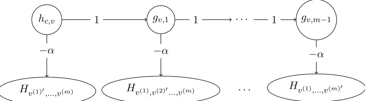
For each hc,v and each 1 ≤ k < m, add an additional hidden unit with 0 bias and no visible-hidden connections. For each hc,v, label thesem−1 hidden unitsg(v,1), ..., g(v,m−1). Since these nodes have no visible-hidden connections they have no effect on the visible distribution at the current time step. For 1 < k < m−1, let w0(v,k),(v,k+1) = 1. Let
w0(c,v),(v,1) = 1 and w(0v,k),j = −α if hj ∈ Hv(t−1),...,v(t−k−1),...,v(t−m) with v(t−k−1) 6= v, and
w0(v,k),j = 0 otherwise (see Fig. 2). Given a sequence v(t−1), ..., v(t−m), consider the prob-ability that h
0(t)
j = 1 for some hidden unit hj ∈Hv(t−1)0,...,v(t−m)0 where v(t−k) 0
6
=v(t−k) for somek. Then by construction there is some hidden nodegk−1 with w0(v,k−1),j =−α. The value of g(kt−−11) is calculated recursively by g(kt−−11) = σ(g(kt−−22)) =σk−1(h(t−k)
c,v(t−k)) =σ
k(0.5β).
Since k is bounded, by making β arbitrarily large we make gk−1 arbitrarily close to 1 and thus make h(jt)0w(0v,k−1),jgk(t−−11) arbitrarily close to −α.
Now suppose we haveh(t)
0
j = 1 for some hidden unit inHv(t−1),...,v(t−m). Then every temporal
connection is−α, andg((v,kt−1)) =σk(−0.5β) for everyg(v,k), so again by makingβ arbitrarily large we make the temporal terms arbitrarily close to 0. Thus as β → ∞, the temporal terms fromh(c,vt−i) are either−α or 0 as needed.
hc,v gv,1 · · · gv,m−1
Hv(1)0,...,v(m) Hv(1),v(2)0...,v(m) · · · Hv(1),...,v(m)0 1
−α
1 1
−α −α
Figure 2: The temporal connections of a control node. Each gv,i connects to
every Hv(1),...,v(i+1),...,v(m) with v(i+1) 0
6
= v and hc,v connects to every Hv(1)0,v(2)...,v(m)
with v(1)0 6=v.
there exist α0, β0 such that α > α0 and β > β0 imply that for all v(t) with t ≥ m,
|Q(v(t)|v(t−1), ..., v(0))−P(v(t)|v(t−1), ..., v(0))|< 0. Note that since the chains are of length
m,Qonly depends on the previousmvisible configurations. Then, once again applying the triangle inequality and continuity of theKL-divergence we can satisfy the first condition of Lemma 1.
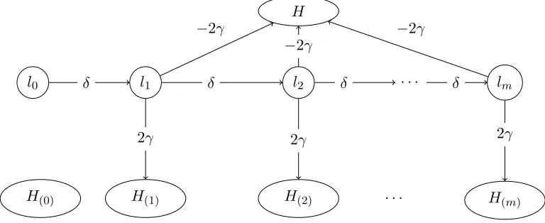
To finish the proof our machine must also be able to approximate the initial m distri-butions. Again this could be easily done should we choose to use an RBM to approximate the distribution of the firstmtime step. Instead we provide a construction to simulate the first m distributions in the RTRBM using the definition given above. As before we will use the construction of Theorem 2 and replace the long-term temporal connections with a chain. To begin, add eachH(i)described in Theorem 2 with the temporal connections again replaced by the chains described in the above step. Now we just need to replace theminitial biases. First add −γ to the bias of each node in H(i). Add hidden units l0, ..., lm−1 with connections between themw(l,i),(l,i+1)=δ and biases −δ forl0, l1 and−0.5δ forl2, ..., lm−1. For everyi >0, define the temporal connections to be 2γ fromli to every node in H(i) and
−2γ to every node inHv(t−1),...,v(t−m) for all v(t−1), ..., v(t−m). Now set the initial biases for everyli to be 0 except forl0. Set this initial bias to be 2δ. Define the initial bias for every other non-control node to be−δwith the exception ofH(0)whose initial bias is 0 (see Fig 3.). First we calculate the values l(it). Since l0 has bias of −δ and initial bias of 2δ, we have
l(0)0 =σ(δ), andl1(1)=σ(δσ(δ)−δ). Taking the limit asδ → ∞we have l(0)0 = 1 and lim
δ→∞l
(1)
1 = limδ→∞σ(δ(σ(δ)−1)) = limδ→∞σ
−δ
1 + exp(δ)
=σ(0) = 0.5.
Next we calculate the limit ofl(2)2 asδ→ ∞:
lim δ→∞l
(2) 2 = lim
δ→∞σ(δl
(1)
1 −0.5δ) = lim δ→∞σ
δ
1 (l(1)1 −0.5)
= lim
δ→∞σ
−(l1(1)−0.5)2 d
dδl (1) 1
!
.
Note that dδdl1(1) is finite and non-zero, so evaluating the limit we get lim δ→∞l
(2)
we have l0(j) = σ(−δ), l1(j+1) = σ(l(0j)−δ) and lk(j+k) = σ(lk(j−+1k−1) −0.5δ) for k > 1. So for j > i we have in the limit that l(ij) = 0. For j < i, we know lj(0)−i ≤ (−0.5δ) so
l(1)j−i+1 = σ(lj(0)−i −0.5δ) , etc., so that in the limit we have lj(i) = 0. We conclude that for any > 0, there exists δ0 such that δ > δ0 implies that for all i > 0 and all j 6= i,
|l0(0)−1|< ,|l(ii)−0.5|< , and |l(ij)|< .
When l(0)0 = 0, li(i) = 0.5, and l(ij) = 0, we have that for t < m, if hj ∈ Hv(t−1),...,v(t−m) orhj ∈H(i) with i6=tthen the bias is at most bj−γ and if hj ∈H(t) then the temporal connections from l1, ..., lm−1 are γ, which cancels the γ subtracted initially so the added bias is 0. For t≥m the temporal connections from li, ..., lm−1 to all Hv(t−1),...,v(t−m) are 0 and the added bias to each node inH(i) is−γ. This is exactly the machine described in the second part of Theorem 2.
Putting this together, we first note that since each li has no visible connections we can ignore their binary values much in the same way that we can ignore the chains in the first part of the proof. Now for t 6= 0 and any > 0 and any v(t), first we choose β > β0 so that |Q(v(t)|v(t−1), ..., v(0))−Q˜(v(t)|v(t−1), ..., v(0))|< 0, then we choose δ > δ
0 so that
|Q˜(v(t)|v(t−1), ..., v(0))−Q¯˜(v(t)|v(t−1), ..., v(0))|< 0 where Q¯˜ is the distribution obtained by
replacingl0(0)with 1,li(i)with 0.5 fori >0, andl(ji) with 0. As noted above this distribution is exactly the construction from the second part of Theorem 2. Finally, by the reasoning of Theorem 1 Step 4, by making δ large we make the initial distribution arbitrarily close to
H(0) allowing us to approximate the distribution for the first time step. So the first, second and third conditions of the lemma are satisfied by the same argument used in Theorem 2.
l1 l2 · · · lm
H(1) H(2) · · · H(m)
H
H(0)
−2γ
δ
2γ
δ δ
2γ 2γ
−2γ
−2γ
l0 δ
Figure 3: The temporal connections of the initial chain. H is the machine
defined in the first part of the proof. Each connection from an li to H or H(k)
only goes to non-control nodes in the set (control nodes include the chains
4. Conclusion
The proofs above have shown that generalized TRBMs and RTRBMs both satisfy the same universal approximation condition. In the proof of universal approximation for the RTRBM we take the weights large enough so that the real-valued hidden sequence becomes approx-imately binary. This suggests that the same proof could be adapted to the basic TRBM. However, the TRBM seems to have difficulty modeling distributions with long term time dependence. After an RTRBM was trained on videos of bouncing balls the machine was able to model the movement correctly and the hidden units contained chains of length two as described in the above proof (Sutskever et al., 2008). On the other hand the TRBM did not have this structure and modeled the motion of balls as a random walk which is what one might expect for a machine that is unable to use velocity data by modeling two-step time dependencies. Given the likely equivalence in representational power of the two models, this discrepancy of results is best explained by the efficiency of the learning algorithm for the RTRBM in comparison to the TRBM.
At first glance the constructions used here seem quite inefficient. For Theorem 1 we require 2n(G(n) + 1) hidden nodes whereGis the number of hidden nodes required to approximate an arbitrary distribution onnnodes with a Restricted Boltzmann Machine. It is important to note that the number of nodes required here, although large, depends only on the number of visible units and the process we wish to approximate, not the number of time steps for which we wish to approximate R. If the required number of hidden nodes had depended on the number of time steps then the TRBM and RTRBM would be essentially pointless as the RBM can do the same for any finite number of time steps. In contrast, the CRBM has a comparatively small lower bound on the number of hidden units required to approx-imate a set of conditional distributions (Montufar et al., 2014). Nonetheless, the above proofs are constructive and give only an upper bound on the required number of hidden units. Furthermore, we made no assumptions about KL(R1(·|v(t−1))||R1(·|v(t−1)
0
)). Even ifv(t−1) andv(t−1)0 are similar vectors, the resulting distributions may be quite different, so to guarantee the result in full generality we could need a whole new set of hidden units to approximate R1 for each pattern v(t−1). With this in mind, we might expect 2n(G(n)) to be a reasonable lower bound. In practice, similar vectors in the previous time step should produce similar distributions for the current time step. For example, looking at consecutive frames in video data, we expect that two similar frames at a certain time step will lead to similar frames in the next time step. To formalize this we could impose the restriction
KL(R1(·|v(t−1))||R1(·|v(t−1) 0
))< f(d(v(t−1), v(t−1)0)), where f is a bounded function andd
is a metric on{0,1}n. With this condition we could hope to find a more efficient TRBM to approximate R than the one given in the proof.
Re-calling the constructions used in the previous proofs, by replacing the RBMs modeling the transition probabilities with Deep Belief Networks we end up with a column structure in which certain control nodes in a column send negative feedback to the other columns. This structure bears an interesting resemblance to the structure of the visual cortex (Goodhill and Carreira-Perpin´an, 2006) suggesting that perhaps the two are computationally similar.
Acknowledgments
Appendix A.
The following table lists notations used for the labels and states for the nodes in the previ-ous proofs
H0 a set of hidden nodes whose distribution approximates R0
H(i) a set of hidden nodes used to approximate the distribution at time i
Hv Hidden nodes whose distribution approximates R1(·|v(t−1) =v)
hc,v the control node corresponding to the configuration v of the visible units
Hc the set of all control nodes
Hc,v(t) the set of configurations of the hidden nodes at time twith hc,v(t) = 1 andh(c,vt)0 = 0 ¯
Hc,v(t) the set of configurations of hidden nodes at time t not in Hc,v(t)
g(v,i) the ith node in a chain connectingh(c,v) to the visible nodes
li the ith node in the initial chain connecting l0 with the rest of the H Appendix B.
In this appendix we provide a proof for Lemma 1
Proof: For an arbitrary >0, we need to find aP ∈P such thatKL(R||P)< , where the KL-divergence is
KL(R||P) =X
vT
R(vT) log
R(vT)
P(vT)
.
We can writeP(vT) as
T−1 Y t=1
P(v(t)|v(t−1), ..., v(0)) !
P(v(0)),
and by assumption
R(vT) = T−1
Y t=m
R1(v(t)|v(t−1), ..., v(t−m)) !m−1
Y i=1
R0(v(i)|(v(i−1), ..., v(0))R0(v(0)).
Then expanding out the log in the KL-divergence gives us
KL(R||P) =X
vT
T−1 X t=m
R(vT) log R1(v
(t)|v(t−1), ..., v(t−m))
P(v(t)|v(t−1), ..., v(0)) !
+X
vT
m−1 X t=1
R(vT) log R0(v
(t)|v(t−1), ..., v(0))
P(v(t)|v(t−1), ..., v(0)) !
+X
vT
R(vT) log R0(v (0))
P(v(0)) !
.
We can decomposeR(vT) intoR(v(T−1), ..., v(t)|v(t−1), ..., v(0))R(v(t−1), ..., v(0)) so for a given
twe can write
X vT
R(vT) log R1(v
(t)|v(t−1), ..., v(t−m))
= X v(t−1),...,v(0)
R(v(t−1), ..., v(0))
×
X v(t)
X v(T−1),...,v(t+1)
R(v(T−1), ..., v(t)|v(t−1), ..., v(0)) log R1(v(t)|v(t−1), ..., v(t−m))
P(v(t)|v(t−1), ..., v(0)) !
= X
v(t−1),...,v(0)
R(v(t−1), ..., v(0))KL(R1(·|v(t−1), ..., v(t−m))||Pt(·|v(t−1), ..., v(0))).
Since R(v(t−1), ..., v(0))<1 for all v(t−1), ..., v(0) we have X
vT
R(vT) log R1(v
(t)|v(t−1), ..., v(t−m))
P(v(t)|v(t−1), ..., v(0)) !
≤2tnX
vt
KL(R1(·|v(t−1), ..., v(t−m))||Pt(·|v(t−1), ..., v(0))). The same logic applies for the cases witht < m.
By hypothesis there existsP ∈Psuch that for every vT and every0,
KL(R1(·|v(t−1), ..., v(t−m))||P
t(·|v(t−1), ..., v(0)))< 0 fort≥m,
KL(R0,t(·|v(t−1), ..., v(0))||Pt(·|v(t−1), ..., v(0)))< 0 for every 0< t < mand
KL(R0||P0)< 0. This gives us
KL(R||P)≤
T−1 X t=m
2tnX vt
KL(R1(·|v(t−1), ..., v(t−m))||Pt(·|v(t−1), ..., v(0)))
+ m−1 X t=1
2tnX vt
KL(R0(·|v(t−1), ..., v(0))||P(·|v(t−1), ..., v(0))) +KL(R0||P0)
<
T−1 X t=m
4tn0+ m−1
X t=0
4tn0.
Then we merely choose an0 so that this expression is less thanand choose a correspond-ingP ∈P.
Notice in the proof that T was chosen arbitrarily and in the last line of the proof we see that decreasing T provides a tighter bound on the KL-divergence so any distribution which approximatesR with a certain upper bound on the KL-divergence for T time steps will approximate R with at most the same upper bound on the KL-divergence for t < T
time steps.
References
G. Goodhill and M. Carreira-Perpin´an. Cortical Columns. Macmillan, first edition, 2006.
G. Hinton. Training a product of experts by minimizing contrastive divergence. Neural Computation, 14:1771–1800, 2002.
Geoffrey E. Hinton and Simon Osindero. A fast learning algorithm for deep belief nets.
Neural Computation, 18:1527–1553, 2006.
N. Le Roux and Y. Bengio. Representational power of restricted Boltzmann machines and deep belief networks. Neural Computation, 20:1631–1649, 2008.
N. Le Roux and Y. Bengio. Deep belief networks are compact universal approximators.
Neural Computation, 22:2192 – 2207, 2010.
G. Montufar and N. Ay. Refinements of universal approximation results for deep belief networks and restricted Boltzmann machines. Neural Computation, 23:1306–1319, 2011.
G. Montufar, N. Ay, and K. Ghazi-Zahedi. Geometry and expressive power of conditional restricted Boltzmann machines. Journal of Machine Learning(Preprint), 2014. URL http://arxiv.org/abs/1402.3346.
I. Sutskever and G. Hinton. Learning multilevel distributed representations for high-dimensional sequences. Proceeding of the Eleventh International Conference on Artificial Intelligence and Statistics, pages 544 – 551, 2006.
I. Sutskever and G. Hinton. Deep, narrow sigmoid belief networks are universal approxi-mators. Neural Computation, 20:2192 – 2207, 2010.
I. Sutskever, G. Hinton, and G. Taylor. The recurrent temporal restricted Boltzmann machine. Advances in Nueral Information Processing Systems, 21:1601–1608, 2008.
G. Taylor, G. Hinton, and S. Roweis. Modeling human motion using binary latent variables.
Advances in Neural Information Processing Systems, 19:1345–1352, 2006.