Comparing Inter-Sensor NDVI for the Analysis of Horticulture Crops in South-Eastern Australia

(1)

Published online March 20, 2014 (http://www.sciencepublishinggroup.com/j/ajrs) doi:110.11648/j.ajrs.20140201.11

Comparing inter-sensor NDVI for the analysis of

horticulture crops in south-eastern Australia

Mohammad Abuzar

1

, Kathryn Sheffield

1

, Des Whitfield

2

, Mark O’Connell

2

, Andy McAllister

2

1

Department of Environment and Primary Industries, 32 Lincoln Square North, Carlton, Victoria3053, Australia 2

Department of Environment and Primary Industries, 255 Ferguson Road, Tatura, Victoria3616, Australia

Email address:

[email protected] (M. Abuzar)

To cite this article:

Mohammad Abuzar, Kathryn Sheffield, Des Whitfield, Mark O’Connell, Andy McAllister. Comparing Inter-Sensor NDVI for the Analysis of Horticulture Crops in South-Eastern Australia.American Journal of Remote Sensing. Vol. 2, No. 1, 2014, pp. 1-9.

doi: 10.11648/j.ajrs.20140201.11

Abstract:

Synergistic application of NDVI from diverse sensors has been an interest of researchers in the field of natural resource management for over two decades. Attempts have been made to deal with the sensor-specific differences in NDVI which stem from a number of factors. In this study, an NDVI comparison has been made between Landsat-7 ETM+ and five other sensors of relatively fine resolution (ASTER, SPOT-5 XS, RapidEye, QuickBird-2 and WorldView-2) over an area of horticultural crops in south-eastern Australia during 2011-12. Translation equations have been developed using linear regression for specific sensors and specific horticultural crops (almond, table grape, wine grape, olive and vegetable). Cross-senor comparisons of NDVI showed strong positive relationships (p <0.001, R2>0.9) but in three cases (ASTER, SPOT-5 and RapidEye) the differences in NDVI values were significant (p<0.001) as well. Though in the other two cases (QuickBird-2 and WorldView-2) the differences were not significant, they were not negligible. Therefore the role of translation equations is considered important for cross-sensor NDVI compatibility. The results of this study will be used: (i) to convert NDVI from the selected sensors to a Landsat- equivalent NDVI for the analysis of irrigated horticultural crops, (ii) to optimise the temporal frequency of NDVI observations for long-term vegetation analyses, and (iii) to transfer Landsat ETM+-based measurements, particularly evapotranspiration (ET) estimates, to alternative sensors that lack thermal band capability which is critical for ET measurements. ET measurements will be used to estimate crop water requirement to help irrigation water management of horticultural crops.

Keywords:

NDVI Comparison, Horticultural Crops, ASTER, SPOT-5, RapidEye, QuickBird-2, WorldView-2

1. Introduction

Normalised difference vegetation index (NDVI) is one of the most widely used measures to assess and monitor vegetation status [1, 2]. Since it was first introduced in 1973 [3], NDVI has been investigated for various applications in a range of agro-climatic conditions, crop types and ecological systems both at the local/field level [4-6] and the regional scale [7-9]. The availability of NDVI data has increased with the launch of many new sensors and satellite systems. The increasing number of sensors has created a need to evaluate and standardise the NDVI data from different available sensors [1, 2, 10]. Inter-sensor comparison of NDVI has been undertaken by a number of researchers for various purposes. The main purpose, however, has been to achieve

data continuity by temporal infill for the monitoring and

modelling of natural resources [2, 10-16].

Factors responsible for inter-sensor NDVI variations are directly related to the two spectral bands (near infrared and red) that form NDVI. These factors can be broadly grouped into the following six categories.

(2)

2 Mohammad Abuzar et al.: Comparing Inter-Sensor NDVI for the Analysis of Horticulture Crops in South-Eastern Australia

minimize the atmospheric effect by selecting images of clear sky conditions.

Second is the effect of solar illumination and viewing angle which is addressed by the application of bi-directional reflectance distribution function (BRDF). Though NDVI values are less sensitive to viewing and solar geometries as compared to the spectral reflectance values that form NDVI [19], it is important to evaluate each situation separately. In this study, we chose only near-nadir satellite images to avoid the need of BRDF calculation. However, we have addressed some aspect of solar geometry in data calibration in this study.

Third is the calibration procedure that may cause inter-sensor NDVI variations. In general, NDVI is calculated using calibrated data sets. Calibration gives precision and correctness to the data from a particular sensor, so that the other data sets from the same sensor are comparable. However, algorithms for calibration, including those for radiometric correction, differ from sensor to sensor, creating some uncertainties when NDVI values from different sensors are compared [16, 20]. Small differences in NDVI have been observed even in very similar sensor systems. For example, a comparison of three very similar sensors (AVHRR from NOAA17, NOAA18 and METOP-A platforms) showed an absolute change in the range of -0.03 and 0.06 NDVI [21]. Some variations can be attributed to modulation transfer function (MTF), including absolute calibration, sun elevation, earth-sun distance, atmospheric conditions and viewing geometry. However, for homogenous surface conditions, MTF effects are negligible [22] and in such cases, sensors may be used interchangeably [23].

Fourth is the lack of bandwidth correspondence, which affects both the value and the dynamic range of NDVI. For example, in a study based on data simulated to represent different sensors (MSS, TM, NOAA-9 AVHRR and SPOT-1 HRV1), the effect of bandwidth showed a low variability among NDVI minima (1.03 - 1.7%) as compared to the NDVI maxima (10.14 -17.12%) [24]. Another study of five simulated bandwidths (10, 30, 50, 100 and 150 nm) showed that an increase in the bandwidth leads to a decrease in NDVI values (from ~ 0.78 to ~ 0.62), with most of the changes attributable to the red band [25].

The fifth includes the differences in spatial and radiometric resolution of sensors. Some studies have shown that coarser spatial resolution images generate higher NDVI values as compared to those with a finer spatial resolution. Though it is not clearly understood as to how differences in spatial resolution affect NDVI in field conditions, several studies have demonstrated this effect while comparing, for example, TM with LISS III [26], ETM+ with IKONOS [27], SPOT with IKONOS [28], and ETM+ with ASTER [10]. Increasing pixel size, however, decreases the spatial variability of NDVI [29]. Another factor that affects NDVI, particularly its dynamic range, is radiometric resolution. Higher bits per data provide higher variability in NDVI [14].

Sixth is the geolocation uncertainty. For inter-sensor

comparisons, it is essential that target surfaces remain the same. Errors due to misregistration of images have been widely reported, for example [30, 31]. In this study we co-registered images to a level of sub-pixel accuracy. Further, we aggregated NDVI pixels within field unit to avoid any further uncertainties due to misregistration.

Though there are multiple factors responsible for inter-sensor differences in NDVI, the management of these differences need not be done on the basis of individual factors. It is rather prudent to deal with the cumulative effect of factors on NDVI. This is why the most popular approach adopted so far is to estimate a transfer function to account for all NDVI differences between sensors which are being compared [13, 28, 32]. In this study we followed the transfer function approach.

There have been previous studies on inter-sensor NDVI differences focused on both mixed [14, 18, 21, 26] and specific [13, 24, 28, 33] land uses. However, studies for horticulture crops are lacking. In this study we attempted to fill this gap by focusing only on horticultural crops in a major fruit-growing region in south-eastern Australia.

NDVI can also be used to help transfer sensor-specific unique information between diverse sensors. Satellites such as Landsat series with thermal capability have distinct advantage of providing information to generate evapotranspiration (ET) [34] but their repeat cycle and spatial resolution may prove limiting in some situations. However, many other sensors lack thermal capability though they are superior in spatial resolution (e.g. SPOT XS and QuickBird) or re-visit frequency (e.g. RapidEye). But almost all available sensors have NDVI as a common capability, which can be used as a medium of information transfer. In this case, Landsat-derived ET estimates can be transferred to other sensors that lack thermal capability, by using NDVI as a medium of transfer.

Ongoing research by the authors of this paper [35-37] and others [38, 39] into satellite-based irrigation water management systems have focused in part on the derivation of land use specific relationships between ET and NDVI, using measurements derived from Landsat TM/ETM+ sensors. These relationships can be used to predict ET based on crop-specific NDVI values and weather data.

(3)

2. Methods

Focus of this study was on horticultural crops in a typical irrigation environment. As horticulture regions are distinct in farm size, crop types and vegetation conditions, compared to the other agricultural land uses, fine resolution images are more suitable for analyses in these areas. Therefore in this investigation, in addition to moderate resolution sensors (SPOT-5 XS, ASTER and Landsat ETM+), we also included high resolution sensors (RapidEye, QuickBird-2 and WorldView

not investigated in much detail in previous studies on inter-sensor NDVI comparison.

Figure 1. Location of study area and extent of satellite images used in the

study. Background is an historical Landsat-7 image as reference.

Satellite / Sensor Spatial resolution(m) Landsat-7 ETM+ 30

Aster Vnir 15 RapidEye 5 QuickBird-2 2.4

SPOT-5 XS 10 WorldView-2 2

All images were co-registered in WGS84 system (Zone 54 S) but their nominal spatial resolutions (Table 2) were maintained. Digital numbers (DN) of each satellite image were converted into radiance using sensor

procedure (Section 2.1). Radiance to reflectance conversion was performed using a uniform procedure as described in Section 2.2. NDVI values were calculated using the reflectance values as described in Section 2.3.

2.1. Conversion to Radiance

2.1.1. Landsat-7 ETM+

The conversion of Landsat-7 ETM+ images into radiance was carried out using the procedure given by Chander et al. [40]:

where

Lλ = Spectral radiance [W/ (m2srµm)]

Qcal= Pixel values (DN)

Qcalmin= Minimum pixel value corresponding to

this study was on horticultural crops in a typical irrigation environment. As horticulture regions are distinct in farm size, crop types and vegetation conditions, compared to the other agricultural land uses, fine resolution nalyses in these areas. Therefore in this investigation, in addition to moderate 5 XS, ASTER and Landsat-7 ETM+), we also included high resolution sensors 2 and WorldView-2), which were detail in previous studies on

Location of study area and extent of satellite images used in the 7 image as reference.

The study area (Fig. 1) is part of the Sunraysia Irr Region of south-eastern Australia, located between 142° 35' 45" E and 143° 20' 28" E longitudes, and between 34° 38' 31" S and 34° 56' 28" S latitudes. The region is dominated by irrigated horticultural crops.

The information on extent and crop ty fields for this study was sourced from

Mapping data sets (www.sunrise21.org.au

represented peak irrigation time for horticultural crops.

Table 1. Satellite images

Image Satellite / Sensor

1 Landsat-7 ETM+

2 ASTER

3 SPOT-5 XS

4 RapidEye

5 Landsat-7 ETM+

6 QuickBird

7 WorldView

The satellite images for this study were selected on the criteria of near-nadir viewing angle and clear sky atmospheric conditions. Two sets of satellite images were selected for Nov-Dec 2011 and Jan 2012 (Table 1).

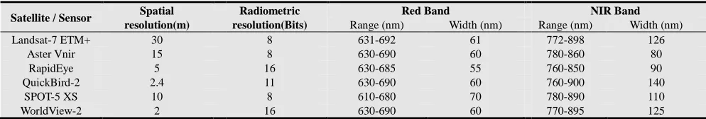
Table 2. Comparison of sensor attributes.

Radiometric resolution(Bits)

Red Band

Range (nm) Width (nm)

8 631-692 61

8 630-690 60

16 630-685 55

11 630-690 60

8 610-680 70

16 630-690 60

registered in WGS84 system (Zone 54 S) but their nominal spatial resolutions (Table 2) were maintained. Digital numbers (DN) of each satellite image were converted into radiance using sensor-specific reflectance conversion was performed using a uniform procedure as described in Section 2.2. NDVI values were calculated using the reflectance values as described in Section 2.3.

ETM+ images into radiance was carried out using the procedure given by Chander et al.

(1)

µm)]

= Minimum pixel value corresponding to

LMINλ [DN]

Qcalmax= Maximum pixel value corresponding to LMAXλ [DN]

LMINλ = Spectral at-sensor radiance scaled to minimum pixel [W/ (m2srµm)]

LMAXλ = Spectral at-sensor radiance scaled to maximum pixel [W/ (m2srµ

The values of Qcalmin, Qcalmax

taken from the metadata file of each scene provided by USGS (http://earthexplorer.usgs.gov/

2.1.2. Aster Vnir

For ASTER image data, the following equation was used to convert DN to radiance [41

Lλ = (Qcal

where UCC is the unit conversion coefficient taken from the ASTER User Handbook

(high, medium or low) of bands. Gain status was taken from the header file of ASTER image.

The study area (Fig. 1) is part of the Sunraysia Irrigation eastern Australia, located between 142° 35' 45" E and 143° 20' 28" E longitudes, and between 34° 38' 31" S and 34° 56' 28" S latitudes. The region is dominated by irrigated horticultural crops.

The information on extent and crop types of horticultural fields for this study was sourced from SunRISE 21 Inc www.sunrise21.org.au). Study period represented peak irrigation time for horticultural crops.

Satellite images used in the study.

Satellite / Sensor Date of acquisition

7 ETM+ 06 Jan 2012

ASTER 06 Jan 2012

5 XS 12 Jan 2012

RapidEye 16 Jan 2012

7 ETM+ 05 Dec 2011

QuickBird-2 13 Dec 2011

WorldView-2 20 Nov 2011

The satellite images for this study were selected on the nadir viewing angle and clear sky atmospheric conditions. Two sets of satellite images were

Dec 2011 and Jan 2012 (Table 1).

NIR Band Range (nm) Width (nm)

772-898 126 780-860 80 760-850 90 760-900 140 780-890 110 770-895 125

Maximum pixel value corresponding to

sensor radiance scaled to minimum

sensor radiance scaled to srµm)]

calmax, LMINλ and LMAXλ were taken from the metadata file of each scene provided by

http://earthexplorer.usgs.gov/).

For ASTER image data, the following equation was used 41]:

-1).UCC (2)

where UCC is the unit conversion coefficient taken from

ASTER User Handbook[41] according to the gains

(4)

2.1.3. RapidEye

Conversion of RapidEye image into radiance was done using the following equation [42]:

Lλ = (Qcal_{-1).RSF (3)}

where RSF denotes radiometric scale factor taken from the header of image file (www.rapideye.com).

2.1.4. QuickBird-2 and WorldView-2

The procedure to convert images to radiance from both satellites is the same. Individual bands were converted into radiance using the following equation [43, 44]:

(4)

where

LλPixel,Band = Spectral radiance per pixel per band [W/ (m2srµm)]

Band

K _{= The absolute calibration factor} [W/ (m2sr count)]

qPixel,Band=Radiometrically corrected image pixels [counts]

∆λ,Band = Effective band width for a given band [µm] The values for the above elements of the Eq. 4 were taken from the header file provided with images.

2.1.5. SPOT-5 XS

To convert DN of SPOT-5 XS image, the following equation was used as recommended by SPOT technical team (http://www.astrium-geo.com/en/40-faq):

Lλ = (X/A) + B (5)

where

X = Digital number [counts] A = Absolute calibration gain B = Absolute calibration offset

2.2. Conversion to Reflectance

The following equation [40] was used to convert radiance to top-of-atmosphere (TOA) reflectance for all the

images:

(6)

where

ρλ = Planetary TOA reflectance [-]

π = Mathematical constant equal to ~3.14159 [-]

Lλ = Spectral radiance [W/ (m2srµm)]

d = Earth-Sun distance [Astronomical units]

ESUNλ= Mean exoatmospheric solar irradiance [W/ (m2µm)]

θs= Solar zenith angle [Degrees]

The sensor-specific values of ESUNλ were taken from

relevant sources given in Table 3.

2.3. Comparative Analysis of NDVI

NDVI values were calculated using the reflectance of red (ρred) and NIR (ρNIR) bands of each image:

NDVI = (ρNIR_-ρred_{) / (}ρNIR₊ρred_{) (7)}

NDVI pixels within the bounds of each selected horticultural field were used to calculate mean NDVI as a representative quantity. The polygons defining field boundaries were buffered 30 m inside to avoid edge effects.

Table 3. Mean exoatmospheric solar irradiance for the near infrared and

red bands of selected sensors.

Satellite / Sensor ESUNλ(W/(m

2_µ_m))

Reference RedBand NIRBand

Landsat-7 1533 1039 [40]

ASTER 1549 1114 [45]

SPOT-5 HRG1 HRG2

1573 1575

1043 1047

ASTRIUM*

RapidEye 1560 1124 RapidEye# QuickBird-2 1575 1114 [43] WorldView-2 1559 1070 [44]

*www2.astrium-geo.com/files/pmedia/ public/r452_9_ normalsolar-irradiance.pdf

#www.rapideye.com/about /resources.htm/ [FAQ]

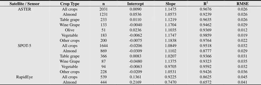
Table 4. NDVI translation equations for horticultural crops (Dependent variable = Landsat-7 ETM+ NDVI.

Satellite / Sensor Crop Type n Intercept Slope R2 _RMSE

ASTER All crops 2031 0.0090 1.1475 0.9676 0.026 Almond 1231 0.0536 1.0573 0.9239 0.026 Table grape 233 0.0110 1.1219 0.9635 0.026 Wine Grape 133 -0.0040 1.1704 0.9462 0.029

Olive 51 0.0236 1.1035 0.9369 0.012

(5)

Satellite / Sensor Crop Type n Intercept Slope R2 _RMSE

Table grape 27 0.0651 1.0462 0.8489 0.053 Wine Grape 13 0.2004 0.8403 0.8937 0.048 Other crops 55 0.1238 0.8823 0.9325 0.035 QuickBird-2 All crops 69 0.0460 0.9600 0.9260 0.049 Table grape 37 0.1051 0.8874 0.8404 0.042 Wine Grape 16 0.0389 0.9789 0.9597 0.036 Other crops 16 0.1240 0.6257 0.9211 0.031 WorldView-2 All crops 162 0.0628 0.9062 0.9405 0.043 Table grape 91 0.0815 0.8767 0.7831 0.044 Wine Grape 37 0.0442 0.9574 0.8925 0.046 Other crops 34 0.1069 0.7098 0.8132 0.033

Two sets of mean NDVI values were created. One was the ‘Jan 2012’ set which included NDVI from Landsat-7 ETM+, ASTER, SPOT-5 and RapidEye (Table 1, images 1-4). The second was the ‘Nov-Dec 2011’ set which included NDVI from Landsat-7, QuickBird-2 and WordView-2 (Table 1, images 5-7). This provided five image comparison cases. Landsat-7 ETM+ NDVI was considered as a dependent variable and NDVI from each of the other five sensors as independent variables.

The areas affected by the scan line correction (SLC) off-mode of Landsat-7 were masked out and not included in this study to avoid any bias in inter-sensor comparison.

A two-sample t-Test (two-tailed, 99% confidence interval) was used to find out whether the two NDVI samples differed significantly from each other. This was done in each of the five bivariate comparison cases.

A series of bilinear regressions were carried out to determine the relationship between two NDVI samples and develop translation equations. Initially, all crop types were considered in one analysis. Subsequently each crop type was analysed separately. Five crop types were identified including almond, tablegrape, wine grape, olive, and vegetable. A sixth category (other crops) included undefined crops and fruit trees.

Intercept, slope, coefficient of determination (R2) and root-mean-square-error (RMSE) were calculated for each comparative analysis.

3. Results

Inter-sensor comparison showed that NDVI varied in value from sensor to sensor. On average, the Landsat-7 ETM+ NDVI was higher than the NDVI from any of the other five sensors. The average value of Landsat-7 ETM+ NDVI was 0.473 whereas the corresponding ASTER NDVI was 0.404, giving an absolute difference of 0.069 which was significant (t-Test, p<0.001). Similar significant differences were found between Landsat7 and SPOT-5 (0.018), and between Landsat-7 and RapidEye (0.105). Differences with QuickBird-2 and WorldView-2 sensors (0.025 and 0.012) were not statistically significant (t-Test, p> 0.01).

The NDVI of each of the selected sensors (ASTER, SPOT-5 XS, RapidEye, Quickbird-2 and WorldView-2) was compared with that of Landsat-7 ETM+ as shown in the scatter diagrams (Figs 2-6). The linear relationship in all cases was highly significant (p<0.001). Minor variations

were observed in the strength of relationship when crop types were considered on an individual basis but statistically they were all highly significant (Table 4).

The relationship between NDVI from ASTER and Landsat-7 ETM+ was very high (R2 = 0.9676), as shown in Fig. 2. The strength of the relationship varied among crop types (Table 4). R2 was the highest (0. 9859) for vegetable and the lowest (0.9239) for almond. RMSE varied between 0.012 and 0.026.

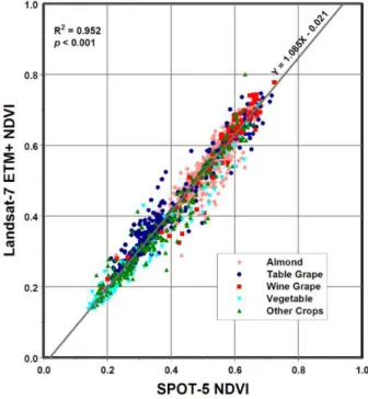
Figure 2. Scatter diagram showing crop-specific mean NDVI values of

Landsat-7 ETM+ and ASTER. Each dots represents a horticultural field.

(6)

A similarly strong relationship (R2 = 0.9518) was found between the SPOT-5 and Landsat-7 ETM+ sensors, as shown in Fig. 3. RMSE was 0.035.

The relationship between NDVI from RapidEye and Landsat-7 ETM+ was relatively low (R2 = 0.8625), as shown in Fig. 4. RMSE ranged between 0.035 and 0.053 (Table 4). The relationship was lower over the almond crops (R2 = 0.6527).

Landsat-7 ETM+ and RapidEye. Each dots represents a horticultural field.

Figure 5. Scatter diagram showing crop-specific mean NDVI of Landsat-7

ETM+ and QuickBird-2. Each dots denotes a horticultural field.

In the case of QuickBird-2 and Landsat-7 ETM+, the NDVI values had a strong significant relationship (R2 = 0.926), as shown in Fig. 5. There were minor variations observed among crop types. RMSE ranged between 0.031 and 0.049 (Table 4). Similarly NDVI from WorldView-2

and Landsat-7 ETM+ showed a strong and significant relationship (R2 = 0.9405) which varied slightly among crop types. RMSE ranged between 0.033 and 0.046 (Table 4).

Figure 6. Scatter diagram showing crop-specific mean NDVI of Landsat-7

ETM+ and WorldView-2. Each dots denotes a horticultural field.

The main results of this study are the parameters of regression equation (intercept and slope) as listed in Table 4, which varied with sensor and crop type. Most equations accounted for more than 90% of the observed variation (R2>0.9), with RMSE ranging between 0.012 and 0.049.

4. Discussion

This study compared the field-scale NDVI of five finer spatial resolution sensors (ASTER, SPOT-5 XS, RapidEye, QuickBird-2 and WorldView-2) against Landsat-7 ETM+ for irrigated horticultural crops.

The images used in this study were near-nadir acquired in clear sky conditions with the assumption that atmospheric corrections and BRDF application were not warranted. However all images were corrected for solar viewing geometries in calibration process. To avoid geolocation uncertainties co-registration of images was carefully carried out and the pixels were aggregated well within the field boundaries. For radiometric correction, a uniform procedure was used to convert from radiance to reflectance. However, the procedure of converting digital number to radiance varied per sensor except between QuickBird-2 and WorldView-2 as described in Section 2.1. There is an emerging research interest in the inter-calibration of satellite instruments [46] which, in future, will reduce or negate the influence of radiometric correction on calculated radiance values.

(7)

near-synchronous images for comparison. For this study, ASTER and ETM+ were acquired on the same day. All other sensors had different acquisitions dates relative to ETM+ but were close enough (≤15 days) for comparison in this context (Table 1). In order to account for the cumulative effect of multiple factors on inter-sensor NDVI, this investigation followed the previous studies [13, 28, 32]in adopting bilinear regression as a method.

The correlations of the inter-sensor NDVIs in all five comparison cases were very high (R2>0.9), statistically significant (<0.001), and positive. Regardless of these close relationships, there were some notable differences in NDVI values observed in both sensor- and crop-specific comparisons.

There are noticeable differences in the spatial resolution of all the sensors compared, ranging between 2 m for QuickBird-2 and 30 m for Landsat-7 (Table 2). Red bandwidths among sensors vary between 55 nm for RapidEye, 62 nm for Landsat-7 ETM+ and 70 nm for SPOT-5. The NIR bandwidths of ASTER (80 nm) and RapidEye (90 nm) differ greatly from Landsat-7 ETM+ (126 nm), whereas those of QuickBird-2, SPOT-5 and WorldView-2 (140, 110, and 125 nm respectively) are closer to Landsat-7 ETM+. In terms of radiometric resolution, Landsat-7 ETM+, ASTER and SPOT-5 are identical (8-bit) while QuickBird-2 is 11-bit and RapidEye is 16-bit.

To deal with differences in spatial resolution, studies on NDVI comparison have adopted two approaches: (1) Pixel-wise approach in which comparisons are made on pixel-by-pixel basis[10, 14, 18, 27] and (2) Representative pixel approach in which comparisons are done by single pixels representative of each unit area [28]. The pixel-wise approach of comparison requires re-sampling of pixels for spatial correspondence. In some cases, re-sampling may introduce some geolocation uncertainties and may require some level of spatial aggregation [18]. Miura et al. [20] recommends an aggregation window of several times larger of original pixel size to compensate for possible misregistration. That approach may not be suitable for certain agricultural fields which are relatively small in size and have different areal shapes. For this study it was considered appropriate to adopt the representative pixel approach where all NDVI pixels within the boundary of each horticultural field were averaged. This approach helps avoid uncertainty due to geolocation.

The published studies on inter-sensor NDVI specific to horticultural crops are lacking, which limits the direct comparison of the findings of this study. However, the studies on the other land uses have investigated various relevant aspects of inter-sensor NDVI comparisons, which have been referred to in the discussion below.

The finding of this study concur with several previous studies [10, 26-28] that sensors with a finer spatial resolution generate lower NDVI values compared with sensors that have a coarser spatial resolution. In this study, Landsat-7 ETM+ NDVI was generally found to be higher compared to the NDVI of the other five sensors, which all had finer

spatial resolution.

Some sensor-specific results of this study are comparable with the findings of previous investigations. Our NDVI relationship between ASTER and Landsat-7 ETM+ (R2 = 0.968, RMSE = 0.026) is marginally stronger than the relationship from Xu and Zhang [10] for a mixed land cover in China (R2 = 0.939, RMSE = 0.057). Soudani et al. [28] investigated the NDVI relationship of Landsat-7 ETM+ and SPOT-4 (which has an identical bandwidth to SPOT-5) for a forested area in France and found R2>0.98, which is slightly higher than our results with SPOT-5 (R2 = 0.952). In a study over Spain for an area of mixed crops, comparing NDVIs of Landsat-7 ETM+ and QuickBird using re-sampled data (25 m, 50 m, 100 m, and 200 m), Martinez-Beltran et al. [18] found varying results (R2 ranging between 0.9495 for 25 m resolution and 0.993 for 200 m) which are slightly higher than our results (R2 = 0.926).

Inter-sensor NDVI relationships investigated in this study were based on the satellite data chosen for the period of peak crop growth and irrigation activities, which is an appropriate timeframe for crop water analysis. Though the data set used in this study was taken from one crop season (2011-12), it represented a range of NDVI values (See Figs 2 – 6) as expected from typical irrigated horticultural crops.

The purpose of this study was to seek an inter-sensor NDVI relationship specific to horticultural crops, which are distinctly different from the other agricultural land uses. It is important to note that the crop-specific differences within horticulture realm do exists and affect NDVI as shown in Table 4 but these differences have been taken into consideration and have been subsumed into the “total crops” category for the derivation of translation equations. The equations for the “total crops” are therefore appropriate to use in mixed horticulture situations.

5. Conclusions

This investigation into an inter-sensor comparison of NDVI of irrigated horticultural crops in the temperate zone of south-eastern Australia provided a set of translation equations to achieve Landsat-equivalent NDVI from five high resolution sensors (ASTER, SPOT-5 XS, RapidEye, QuickBird-2 and WorldView-2). These equations are based on the statistically strong (R2> 0.9) and significant (p <0.001) relationships of inter-sensor NDVI measures, suggesting sufficient confidence in their use for typical irrigated horticultural crops. These translation equations will be used to derive Landsat-equivalent NDVI and transfer Landsat based measurement of ET to alternative sensors. The ET estimates thus achieved will be used in estimating crop water requirement to help routine irrigation water management of horticultural crops in south-eastern Australia.

Acknowledgement

(8)

(http://earthexplorer.usgs.gov/). RapidEye image data was provided by SunRISE 21 Inc., Mildura. Image data of WorldView-2 and QuickBird-2 was provided by Murray Valley Winegrowers Inc., Mildura.

References

[1] Miura, T., A. Huete, and H. Yoshioka, An empirical investigation of cross-sensor relationships of NDVI and red/near-infrared reflectance using EO-1 Hyperion data. Remote Sensing of Environment, 2006. 100(2): p. 223-236. [2] Miura, T., J.P. Turner, and A.R. Huete, Spectral compatibility

of the NDVI across VIIRS, MODIS, and AVHRR: An analysis of atmospheric effects using EO-1 Hyperion. IEEE Transactions on Geoscience and Remote Sensing, , 2013. 51(3): p. 1349-1359.

[3] Rouse, J.W., Haas, R. H,, Schell, J. A., Deering, D. W., Monitoring vegetation systems in the Great Plains with ERTS, Third ERTS Symposium1973, NASA SP-351 I: Washington, DC. p. 309-317.

[4] Hatfield, J.L. and J.H. Prueger, Value of using different vegetative indices to quantify agricultural crop characteristics at different growth stages under varying management practices. Remote Sensing, 2010. 2(2): p. 562-578.

[5] Rossini, M., et al., High resolution field spectroscopy measurements for estimating gross ecosystem production in a rice field. Agricultural and Forest Meteorology, 2010. 150(9): p. 1283-1296.

[6] Marti, J., et al., Can wheat yield be assessed by early measurements of Normalized Difference Vegetation Index? Annals of Applied Biology, 2007. 150(2): p. 253-257. [7] Gu, Y., B.K. Wylie, and N.B. Bliss, Mapping grassland

productivity with 250-m eMODIS NDVI and SSURGO database over the Greater Platte River Basin, USA. Ecological Indicators, 2013. 24(0): p. 31-36.

[8] Mkhabela, M.S., et al., Crop yield forecasting on the Canadian Prairies using MODIS NDVI data. Agricultural and Forest Meteorology, 2011. 151(3): p. 385-393.

[9] Jiang, Z., et al., Analysis of NDVI and scaled difference vegetation index retrievals of vegetation fraction. Remote Sensing of Environment, 2006. 101(3): p. 366-378.

[10] Xu, H. and T. Zhang. Comparison of Landsat-7 ETM+ and ASTER NDVI measurements. In:Tong et al. (Ed.), Remote Sensing of the Environment: The 17th China Conference on Remote Sensing. 2011. Proc. of SPIE vol. 8203 82030K-1. [11] Ambinakudige, S., J. Choi, and S. Khanal, A comparative

analysis of CBERS-2 CCD and Landsat-TM satellite images in vegetation mapping. RevistaBrasileira de Cartografia 2010. 63(1): p. 115-122.

[12] Brown, M., Pinzón, JE, Didan, K, Morisette, JT, Tucker, CJ, Evaluation of the Consistency of Long-Term NDVI Time Series Derived From AVHRR, SPOT-Vegetation, SeaWiFS, MODIS, and Landsat ETM+ Sensors. IEEE Transactions on Geoscience and Remote Sensing, 2006. 41(7 Part 1): p. 1787 - 1793.

[13] Steven, M.D., et al., Intercalibration of vegetation indices from different sensor systems. Remote Sensing of Environment, 2003. 88(4): p. 412-422.

[14] Thenkabail, P.S., Inter-sensor relationships between IKONOS and Landsat-7 ETM+ NDVI data in three ecoregions of Africa. International Journal of Remote Sensing, 2004. 25(2): p. 389-408.

[15] van Leeuwen, W.J.D., et al., Multi-sensor NDVI data continuity: Uncertainties and implications for vegetation monitoring applications. Remote Sensing of Environment, 2006. 100(1): p. 67-81.

[16] Yin, H., et al., How normalized difference vegetation index (NDVI) trends from Advanced Very High Resolution Radiometer (AVHRR) and SystemeProbatoired'Observation de la Terre VEGETATION (SPOT VGT) time series differ in agricultural areas: An inner Mongolian case study. Remote Sensing, 2012. 4(11): p. 3364-3389.

[17] Chavez, P.S., Image-based atmospheric corrections - Revisted and improved. Photogrammetric Engineering and Remote Sensing, 1996. 62(9): p. 1025-1036.

[18] Martinez-Beltran, C., et al., Multisensor comparison of NDVI for a semi-arid environment in Spain. International Journal of Remote Sensing, 2009. 30(5): p. 1355-1384. [19] Gao, F., et al., Bidirectional NDVI and atmospherically

resistant BRDF inversion for vegetation canopy. IEEE Transactions on Geoscience and Remote Sensing, 2002. 40(6): p. 1269-1278.

[20] Miura, T., et al., Inter-Comparison of ASTER and MODIS surface reflectance and vegetation index products for synergistic applications to natural resource monitoring. Sensors, 2008. 8(4): p. 2480-2499.

[21] Trishchenko, A.P., Effects of spectral response function on surface reflectance and NDVI measured with moderate resolution satellite sensors: Extension to AVHRR NOAA-17, 18 and METOP-A. Remote Sensing of Environment, 2009. 113(2): p. 335-341.

[22] Guyot, G. and X.-F. Gu, Effect of radiometric corrections on NDVI-determined from SPOT-HRV and Landsat-TM data. Remote Sensing of Environment, 1994. 49(3): p. 169-180. [23] Gallo, K.P. and J.C. Eidenshink, Differences in visible and

near-IR responses, and derived vegetation indices, for the NOAA-9 and NOAA-10 AVHRRs. Photogrammetric Engineering and Remote Sensing 1988. 54(4): p. 485-490. [24] Gallo, K.P. and C.S.T. Daughtry, Differences in vegetation

indices for simulated Landsat-5 MSS and TM, NOAA-9 AVHRR, and SPOT-1 sensor systems. Remote Sensing of Environment, 1987. 23(3): p. 439-452.

[25] Teillet, P.M., K. Staenz, and D.J. William, Effects of spectral, spatial, and radiometric characteristics on remote sensing vegetation indices of forested regions. Remote Sensing of Environment, 1997. 61(1): p. 139-149.

[26] Anderson, J.H., et al., Intercalibration and Evaluation of ResourceSat-1 and Landsat-5 NDVI. Canadian Journal of Remote Sensing, 2011. 37(2): p. 213-219.

(9)

[28] Soudani, K., et al., Comparative analysis of IKONOS, SPOT, and ETM+ data for leaf area index estimation in temperate coniferous and deciduous forest stands. Remote Sensing of Environment, 2006. 102: p. 161-175.

[29] Tarnavsky, E., S. Garrigues, and M.E. Brown, Multiscalegeostatistical analysis of AVHRR, SPOT-VGT, and MODIS global NDVI products. Remote Sensing of Environment, 2008. 112(2): p. 535-549.

[30] Townshend, J.R.G., et al., The impact of misregistration on change detection. IEEE Transactions on Geoscience and Remote Sensing, 1992. 30(5): p. 1054-1060.

[31] Verbyla, D.L. and S.H. Boles, Bias in land cover change estimates due to misregistration. International Journal of Remote Sensing, 2000. 21(18): p. 3553-3560.

[32] Hill, J. and D. Aifadopoulou, Comparative analysis of landsat-5 TM and SPOT HRV-1 data for use in multiple sensor approaches. Remote Sensing of Environment, 1990. 34(1): p. 55-70.

[33] Maselli, F., Monitoring forest conditions in a protected Mediterranean coastal area by the analysis of multiyear NDVI data. Remote Sensing of Environment, 2004. 89(4): p. 423-433.

[34] Allen, R., et al., Satellite-based ET estimation in agriculture using SEBAL and METRIC. Hydrological Processes, 2011. 25(26): p. 4011-4027.

[35] O’Connell, M.G., et al., Satellite Remote Sensing of water use and vegetation cover to derive crop coefficients for crops grown in Sunraysia Irrigation Region of Victoria, Australia. Acta Horticulturae, 2011. 889: p. 543-549.

[36] Abuzar, M., et al., Satellite-based measurements for benchmarking regional irrigation performance in Goulburn-Murray Catchment. International Archives of the Photogrammetry, Remote Sensing and Spatial Information

Sciences, 2012. XXXIX-B8: p. 221-223.

[37] Whitfield, D.M., et al., SEBAL-METRIC estimates of crop water requirement in horticultural crops grown in SE Australia. Acta Horticulturae, 2011. 922: p. 141-148. [38] Tasumi, M., et al., Satellite-Based Energy Balance to Assess

Within-Population Variance of Crop Coefficient Curves. Journal of Irrigation and Drainage Engineering, 2005. 131(1): p. 94-109.

[39] Tasumi, M. and R.G. Allen, Satellite-based ET mapping to assess variation in ET with timing of crop development. Agricultural Water Management, 2007. 88(1-3): p. 54-62. [40] Chander, G., B.L. Markham, and D.L. Helder, Summary of

current radiometric calibration coefficients for Landsat MSS, TM, ETM+, and EO-1 ALI sensors. Remote Sensing of Environment, 2009. 113(5): p. 893-903.

[41] Abrams, M., S. Hook, and B. Ramachandran, ASTER User Handbook, Version 2, 2002, JPL, NASA.

[42] RapidEye, RapidEye Standard Image Product Specifications2009, Germany.

[43] Krause, K., Radiometric Use of QuickBird Imagery - Technical Note2005: DigitalGlobe, Longmont, Colorado, USA.

[44] Updike, T. and C. Comp, Radiometric Use of WorldView-2 Imagery2010: DigitalGlobe Inc.

[45] Thome, K.J., S.F. Biggar, and P.N. Slater, Effects of assumed solar spectral irradiance on intercomparisons of Earth-observing sensors. Proceedings SPIE 2001. 4540: p. 260-269.