Efficient Computation of Gapped Substring Kernels
on Large Alphabets
Juho Rousu [email protected]
Department of Computer Science Royal Holloway University of London Egham, TW20 0EX, United Kingdom
John Shawe-Taylor [email protected]
School of Electronics and Computer Science University of Southampton
Southampton, SO17 1BJ, United Kingdom
Editor: Tommi Jaakkola
Abstract
We present a sparse dynamic programming algorithm that, given two strings s and t, a gap penalty λ, and an integer p, computes the value of the gap-weighted length-p subsequences kernel. The al-gorithm works in time O(p|M|log|t|), where M={(i,j)|si=tj}is the set of matches of characters in the two sequences. The algorithm is easily adapted to handle bounded length subsequences and different gap-penalty schemes, including penalizing by the total length of gaps and the number of gaps as well as incorporating character-specific match/gap penalties.
The new algorithm is empirically evaluated against a full dynamic programming approach and a trie-based algorithm both on synthetic and newswire article data. Based on the experiments, the full dynamic programming approach is the fastest on short strings, and on long strings if the alphabet is small. On large alphabets, the new sparse dynamic programming algorithm is the most efficient. On medium-sized alphabets the trie-based approach is best if the maximum number of allowed gaps is strongly restricted.
Keywords: kernel methods, string kernels, text categorization, sparse dynamic programming
1. Introduction
Machine learning algorithms working on sequence data are needed both in bioinformatics and text categorization and mining. In contrast, standard machine learning algorithms work on feature vector representation, thus requiring a feature extraction phase to map sequence data into feature vectors.
Representing these feature vectors explicitly is often problematic due to the potentially high dimensionality. Kernel methods (Vapnik, 1995; Cristianini and Shawe-Taylor, 2000) provide an ef-ficient way of tackling the problem of dimensionality via the use of a kernel function, corresponding to the inner product of two feature vectors. With these precomputed inner products, it is possible to efficiently accomplish a variety of machine learning and data analysis tasks, e.g. classification, regression and clustering.
The family of kernel functions defined on feature vectors computed from strings, are called
string kernels (Watkins, 2000; Haussler, 1999). These kernels are based on features corresponding
can have bounded or unbounded length, and the mismatches or gaps can be penalized in different ways.
There are three main approaches in computing string kernels efficiently. Dynamic programming approaches (Lodhi et al., 2000; Cancedda et al., 2003) are based on composing the solution from simpler subproblems, in this case, from kernel values of shorter subsequences and prefixes of the two strings. These approaches usually have time complexity of orderΩ(p|s||t|)since one typically needs to compute intermediate results for each character pair si,tj for each subsequence length 1≤l≤ p. However, there is no extra computational cost associated when using gap penalties
or mismatch costs between the characters. In trie-based approaches (Leslie et al., 2003; Leslie and Kuang, 2003) one makes a depth-first traversal to an implicit trie data structure. The search continues along each trie path while in both of the strings there exist an occurrence of the p-gram corresponding to the trie node. This termination condition prunes the search space very efficiently if the number of gaps is restricted enough. The third approach is to build a suffix tree of one of the strings and then compute matching statistics of the other string by traversing the suffix tree to compute matching statistics (Vishwanathan and Smola, 2003). The computation of the kernel value takes a linear time. However, the approach does not deal with gapped strings.
In this paper, we concentrate on improving the time-efficiency of the dynamic programming ap-proach to gapped string kernel computation. In Section 2 we review types of kernels that are used in text categorization and sequence analysis tasks. As a full review of kernel based machine learning is not possible in the context of this article, a reader not familiar with kernel methods might want to refer to the introductory text book of Cristianini and Shawe-Taylor (2000) or, for a more broad treat-ment, the books by Sch¨olkopf and Smola (2001) and Shawe-Taylor and Cristianini (2004). In Sec-tion 3, we review trie-based and a dynamic programming approaches for gap-weighted string kernel computation before presenting the main contribution of this article, a sparse dynamic programming algorithm for efficiently computing the kernel on large alphabets. We also discuss variants and im-plementation of the algorithm. In Section 4 the new algorithm is experimentally compared against the full dynamic programming approach and a trie-based algorithm. Results and open problems are discussed in Section 5 followed by conclusions in Section 6.
2. Kernels for Sequence Data
Kernel methods encompass a family of pattern analysis methods that share a common aspect: map-ping the inputs x∈X to some potentially high-dimensional feature space
F
by defining a feature map φ: X 7→F
, and then solving the pattern analysis task by linear methods, such as finding a separating hyperplane for instances of different classes (support vector machines, SVM), or find-ing principal components of the feature vectorsφ(x)(kernel PCA), or finding correlations between two viewsφ1(x),φ2(x)of the same data (kernel canonical correlation analysis, KCCA). Working in these high-dimensional spaces in made possible by the use of the so called ’kernel trick’: one does not need to handle the feature vectors explicitly, as long as the inner product, the kernel,K(x,z) =φ(x)Tφ(z)has been computed.
a quadratic programme
max αi≥0
∑
iαi−1/2
`
∑
i,j=1
αiαjyiyjK(xi,xj)s.t.
∑
iαiyi=0,
and the SVM prediction can be expressed as f(x) =sign(∑iαiyiK(xi,x) +b). Thus, the learning and prediction can be performed in space that has dimension in the order of the number of the training points.
When handling input data that already comes in vector form, there is no obligation to introduce a special kernel function. The inner product of the inputs K(x,z) =xTz, also called the ’linear kernel’, can be used. However, when using structured data such as sequences, trees or graphs, one needs to convert the structured representation to a vector form.
For sequences the most common feature representation is to count or check the existence of sub-sequence occurrences, when the subsub-sequences are taken from a fixed index set U . Different choices for the index set and accounting for occurrences give rise to a family of feature representations and kernels. Below we review the main forms of representation for sequences and the computation kernels for such representations.
Word spectrum (Bag-of-words) kernels. In the most widely used feature representation for strings in a natural language, informally called bag-of-words (BoW), the index set is taken as the set of words in the language, possibly excluding some frequently occurring stop words (Salton et al., 1975). The representation was brought to SVM learning by Joachims (1998).
In the case of a string s containing English text, for each English word u, we define the feature value
φu(s) =|{j|sj. . .sj+|u|−1=u}|, (1) as the number of times u occurs in some position j of s. For the example text s= ’The cat
was chased by the fat dog’ the BoW will contain the following non-zero entries:φthe(s) =2,
φdog(s) =1,φwas(s) =1,φchased(s) =1,φby(s) =1,φfat(s) =1,φcat=1. These occurrence counts
can also be weighted, for example by scaling by the inverse document frequency (TFIDF, Salton & Young, 1973):
φu(s) =|{j|sj. . .sj+|u|=u}| ×log2N/Nu,
where Nuis the number of documents where u occurs and N is the total number of documents in the collection.
Although the dimension of the feature space may be very high, computation of the BoW kernel can be efficiently implemented by scanning the two strings, constructing lists L(s)and L(t)of pairs (u,cu)of word u and occurrence count cuordered in the lexicographical order of the substrings u, and finally traversing the two lists to compute the dot product.
Substring spectrum kernels. For strings that do not encompass a crisply defined word-structure, for example, biological sequences, a different approach is more suitable. Given an alphabetΣ, a simple choice is to take U=Σp, the set of strings of length p. The featuresφ
u(s),u∈Σpare then defined as in (1). For example, if we choose p=4 resulting feature values for our example text includeφthe =2,φthe=1,φcat=1,φdog=1, along with close to thirty additional 4-grams.
subsequences vary within a range:
U=Σq∪Σq+1· · · ∪Σpfor some 1≤q≤p. (2)
We call the resulting kernel the bounded-length substring kernel. In our example text, we could set q=3 and p=5 to include features such asφdog,φchase andφ f at , for instance. In the extreme case, we can take p=1 and q=∞, thus including in the index set all non-empty sequences of alphabet Σ. It should be noted that the choice of parameters q and p has several effects: First, as will be discussed in the next section, the time to compute the kernels will increase by increasing p. Secondly, if all important subsequences have length at least some q0, setting q<q0 will probably make the spectrum more ’noisy’. Similarly, setting q0<q will probably lose some of the ’signal’. An interesting direction, that is out of scope of this paper, would be to learn the parameters p and q from the data.
The most efficient approaches, working in O(p(|s|+|t|))time, to compute substring spectrum kernels are based on suffix trees (Leslie et al., 2002; Vishwanathan and Smola, 2003), although dynamic programming and trie-based approaches also can be used.
Gapped substring spectrum kernels. Another way to add flexibility to our feature representation is to allow gaps in the subsequence occurrences. In that case, the index set of (2) can still be used but the definition of the features changes. For convenience of notation, in the following we will use boldface letters to indicate ordered collections of indices: j= (j1,j2, . . . ,jq),j1< j2<· · ·<
jq and denote s(j) =sj1. . .sjq. We define the features φu(s) to count the number of such unique
sequences of indices j that the corresponding subsequence sj1. . .sjq equals to u, in other words
φu(s) =|{j|s(j) =u}|.Our example string’The cat was chased by the fat dog’can be seen to contain, among others, the following gapped substrings of length 3:φtea=7,φted=5,φdog=2.
This definition does not make a difference between occurrences that contain few gaps and those that contain several gaps, or the lengths thereof; all contribute to the feature value equally. For example, the substring ’tea’ will have a high weight as it occurs many times in the text, although it never occurs with fewer than two gaps and the total length of gaps is at least three. At the same time, ’dog’ will have much smaller weight although it occurs in the text without any gaps.
A solution for this problem is to downweight occurrences that contain many or long gaps. Such feature representation is the basis of gap-weighted string kernels. In string matching, there are many approaches for weighting gaps (see e.g. Eppstein, 1989; Gordon et al., 2003). We consider two gap-weighting schemes, both of which downweight occurrences exponentially in increasing gap number or length.
When downweighting by the total length of gaps the weight of an occurrence i= (i1, . . . ,iq) with span span(i) =iq−i1+1 is defined asλspan(i), where 0<λ≤1 is a fixed penalty constant. The feature values are then defined as a normalized sum of occurrence weights
φu(s) =1/λq
∑
i:u=s(i)
λspan(i).
The normalization 1/λqensures that only gaps—not matches—are penalized. This normalization is important when using substrings of different lengths as the index set
U
, otherwise short substrings easily get too much weight.be computed will then be
φu(s) =
∑
i:u=s(i)
λ∑jJij+1−ij>1K,u∈Σp,
where the expression inside the indicator function J·K counts pairs of adjacent indices (ij,ij+1) within i where there’s a gap in between the two indices.
In literature, two approaches for computing gapped substring kernels appear, a dynamic pro-gramming approach (Lodhi et al., 2002) and a trie-based approach (Leslie et al., 2002), both of which can deal with gap-weighting as well. We review the dynamic programming approach and a variant of the trie-based computation in Section 3, followed by a presentation of the new sparse dynamic programming approach.
Generalized alphabets. We conclude this section by noting that treating text as strings of charac-ters is not the only and not necessarily the best approach. Depending on the application, considering larger units such as syllables (c.f. Saunders et al., 2002) or words (c.f. Cancedda et al., 2003) may be beneficial. Using the text ’The cat was chased by the fat dog’ as the example, if words are used as the alphabet:
• Substrings are word sequences, or phrases: ’cat was chased’.
• Gapped substrings will be phrases with some words skipped: ’cat ? chased ? ? ?
dog’.
• Penalizing gaps will decrease the weight of phrases that span too long a text segment. For example, the weight of ’cat was chased’ would be higher than that of ’cat ? chased ? ? ? dog’ as the former phrase exists in the text as such whereas the latter contains two gaps of total length four.
Using phrases as features has a potential advantage over the bag-of-words representation, as the ordering and the proximity of the words is taken into account. Thus such a representation should be able to more closely capture syntactically and, ideally, semantically similar text segments.
There is, however, one drawback in using words or phrases as the features, namely the slight variations in the word occurrences that still correspond to the same meaning. Such variations in-clude alternative spellings, prefixes/suffixes attached to words or word stems. These problems can of course be tackled by preprocessing the documents. An alternative approach is the use of sylla-ble alphabet: the text is treated as a sequence of syllasylla-bles: ’The cat was cha sed by the fat dog’. The benefit is that small spelling variations or inflection of the word (e.g. ’cha se’ vs. ’cha sed’) are likely to retain some of the original syllables.
Compared to the character alphabet, word and syllable alphabets share two benefits. Firstly, as argued above, using phrases of words or syllables are more likely to capture meaning in the text than arbitrary substring of characters. Secondly, as the document size drastically goes down when moving from character to syllable and word alphabets, computational requirements decrease as well.
3. Computing Gap-Weighted String Kernels
Let us now concentrate to the question how to efficiently compute the gap-weighted string kernel:
K(s,t) =
∑
u∈UA (’the’,g)s A (’the’,g)t A (’the dog’,g)s A (’the dog’,g)t
2 2 2 2
3 3 3 3
5 5 5 5
cat
the
dog
dog
fat
cat
the
fat
dog
dog
dog
dog
the
dog
the
dog
dog
g g g g
0 0 0 0
1 1 1 1
4 4 4 4
6 6 6 6
{1,6} {1,5}
{8}
{8}
{6}
{6}
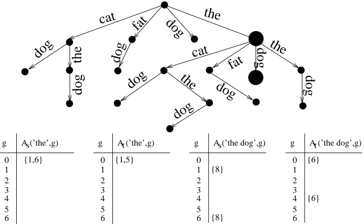
Figure 1: The co-occurrence trie of the example strings (top), and the sets of alive indices for the substrings ’the’ and ’the dog’ in the two strings with numbers of gaps ranging from 0 to 6 (bottom).
where the index set satisfies U=Σpor U=Σq∪. . .Σp, and
φu(s) =1/λp
∑
i:u=s(i)
λspan(i) (4)
We will present three algorithms all of which are then experimentally compared in Section 4. The first is based on constructing an implicit trie data structure for the co-occurring gapped substrings in s and t. The second algorithm is the dynamic programming approach by Lodhi et al., (2002), and the third is a new method based on sparse dynamic programming.
As a running example we we use two strings s=’The cat was chased by the fat dog’ and t =’The fat cat bit the dog’ and, for illustration, we apply the word alphabet. Hence, in the example, ’letters’ corresponds to English words, ’substrings’ and ’subsequences’ to English phrases.
3.1 Trie-Based Computation
Thus the resulting kernel can be considered as an approximation of (3) where co-occurrences with mor than gmaxgaps are discarded.
Figure 1 shows the trie structure of co-occurring subsequences for the example strings, when the index set is fixed to U =Σ3, the three word phrases. Below we briefly describe a trie-based algorithm that is a slight variation of the one described by Shawe-Taylor and Cristianini (2004) and also bear resemblance to the related mismatch string kernel algorithm by Leslie et al. (2003).
In a trie-node corresponding to subsequence u=u1· · ·uqthe algorithm keeps track of all matches
s(i) =u that could still be extended further. For each such index set i=i1. . .iq, the last index iqis stored in a list of alive matches As(u,g)where g=span(i)−q is the number of gaps in the match. Similarly for t the lists At(u,g) are maintained. To expand a node u, the algorithm looks for all possible letters the matching subsequence can be extended to a longer match uc. For an alive match
i∈As(u,g)and all g0≤gmax−g the algorithm puts the indices i+1+g0 into As(usi+1+g0,g+g0).
The lists At(uti+1+g0,g+g0)are constructed the same way. The search is continued for nodes uc
for which both S
gAs(uc,g)
and S
gAt(uc,g)
are non-empty, that is, there is at least one occur-rence of uc in both s and t, with some number of gaps. This makes the trie much sparser than the subsequence tries for either one of the strings alone would be.
In our example (Figure 1), ’the’ is encountered in positions 1 and 6 of s, with (trivially) no gaps, and in positions 1 and 5 in t. To find the alive indices for ’the dog’ the algorithm searches for the occurrence of ’dog’, in s from indices 2 and 7 onwards, and finds the occurrence in position 6, corresponding to an occurrence with 1 and 4 gaps, respectively. Similar analysis is performed for
t. When a node u in depth d is encountered one easily obtains the relevant terms in the kernel via
computing the sum
φu(s)φu(t) =
∑
gs,gtλgs+d|A
s(u,gs)| ·λgt+d|At(u,gt)|.
If a length-p subsequence kernel is being computed this computation only need to be performed in the leaves of the trie. For bounded-length subsequence kernel, the computation needs to be performed in all trie nodes that are in depth q≤d≤p.
Note that the above approach differs from the(g,k)-gapped trie algorithm by Leslie and Kuang (2003) in two respects: First, the strings s and t are not broken into frames before the search but the algorithm maintains the lists As(u,g)to keep track of the subsequence occurrences. Second, the algorithm keeps track of the number of gaps in the occurrences during the search. This relieves us from the need to embark on dynamic programming search in the trie leaves to compute the values
φu(s)φu(t).
The worst-case time complexity of the algorithm, O( p+gmax
p
(|s|+|t|)), arises when s=t, which
follows from noticing that each position in the two strings is a start location of a co-occurring subsequence, and there are O( p+gmax
p
)possible combinations of assigning p letters and gmaxgaps in a window of length p+gmax. Note that if no gaps are allowed we get the time complexity
O(p(|s|+|t|)matching the suffix tree approach.
3.2 Dynamic Programming Computation
The basis of dynamic programming computation of the string kernel (3) is the following observation: if there is a co-occurrence of substring u1. . .uqthat ends in positions k’th and l’th position of s and
t, respectively, two conditions must be satisfied:
λ5
λ4
+
λ8λ11
λ2 λ2
λ2
λ2
λ2
λ2 λ2
the was chased by the fat
the
the bit fat
cat dog
cat
dog the was chased by the fat
the
the bit fat
cat dog
cat
dog 1
κ
2
κ
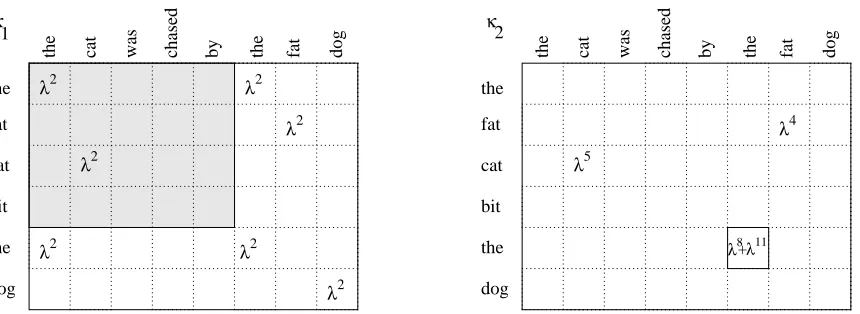
Figure 2: The co-occurrence weights of length-one (a) and length-two (b) substrings. Computing
κ2(6,8)requires efficiently maintaining the appropriately scaled sum of the weights in the shaded region ofκ1.
2. there must be a matching prefix u1. . .uq−1 that ends in some position i<k in string s and some position j<l in string t.
Moreover, ignoring the normalization 1/λ2q, the co-occurrence weight can be computed by from the weight of the prefix co-occurrence by extending the subsequences with k−i and l−j letters,
respectively:
λspan([i1...,iq,k])·λspan([j1...,jq,l])=λspan([i1...,iq])·λspan([j1...,jq])·λk−iqλl−jq.
Denoting byκq(k,l) the sum of weights of length-q substring co-occurrences, again ignoring the normalization 1/λ2q, that end at positions k and l in s and t, respectively, the above observations can be summarized in the following recurrence
κq(k,l) =
(
λ2Js
k=tlK for q=1, and
∑i<k∑j<lλk−i+l−jκq−1(i,j)Jsk=tlK, for q>1,
(5)
where Figure 2 depicts the idea behind the recurrence (5): to computeκ2(5,6)we need to extend the length-1 matches in the shaded region,κ1(i,j),i<5,j<6, into length-2 matches by adding gaps. The weights of two length-1 matches in positions(1,1) and(3,2)are rescaled before summation:
λ8+λ11=λ5−3+6−2λ2+λ5−1+6−1λ2.
The dynamic programming algorithm (Figure 4) computes this recurrence by starting with sub-sequence length 1, which requires looping through all pairs of positions (i,j) in the two strings, checking for matching letters and summing up the co-occurrence weights. For convenience, the algorithm computes the sum of weights without the normalization 1/λ2qthat is applied in the final phase when computing the kernel value K(q).
Longer subsequences are handled in increasing order of length, in accordance to (5). How-ever, computing the double sum for each(k,l)(e.g. the shaded region in Figure 2) would be very inefficient, hence instead, a separate table storing the double sum
S(k,l) =
∑
i<k∑
j<lλk−i+l−jκ
κ1
λ
2λ
2λ
2λ
2λ
2 λ2λ3 λ4
λ5
λ
6λ4
λ3 λ5 λ6 λ7
λ6+λ9
λ2
+λ5
λ4
λ5
λ3+λ6 λ4+λ7λ5+λ8
λ3+λ6 λ5
+λ8
λ4+λ7
the was chased by the fat
the the bit fat cat dog cat dog S the was chased by the fat
the the bit fat cat dog cat dog
λ
2λ
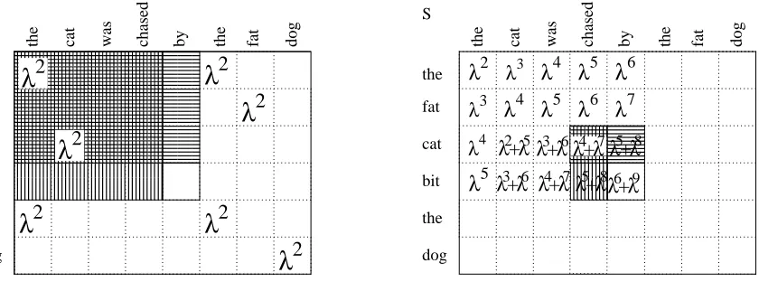
2Figure 3: The table S (right) stores the scaled sums of co-occurrence weights of the prefixes of the strings. The value S(k,l)is computed in constant time by adding upκq−1(k,l)λS(k−1,l) (horizontally striped area) andλS(k,l−1) (the vertically striped area) and subtracting
λ2S(k−1,l−1)(the intersection) that would otherwise be doubly counted.
is maintained. With that auxiliary table, computing the recurrence is very simple
κq(k,l) =Jsk=tlKλ2S(k−1,l−1). Maintenance of the table S can be done efficiently via the relationship
S(k,l) =κq−1(k,l) +λS(k−1,l) +λS(k,l−1)−λ2S(k−1,l−1), (6) where the first term computes the contribution of the cell (k,l), the two middle terms the regions
{(i,j)|i<k,j≤l}and{(i,j)|i≤k,j<l}, respectively, and the last term subtracts the twice counted region{(i,j)|i<k,j<l}.
In Figure 3 the computation of the value S(4,5) =λ6+λ9is depicted. The value can be seen as the sum of weights of matching ’the ? ? ?’ with ’the ? ? ? ?’ (weightλ4·λ5) and ’the’ (λ3·λ), and ’cat’ with ’cat ? ? ? ?’ (weightλ·λ5).
The algorithm has time complexity O(p|s||t|)which is immediately seen from the pseudocode in Figure 4. It is possible to optimize the algorithm to consume less memory. As the computation proceeds in increasing order of subsequence length and only the previous length is referred to, it suffices to maintain a single tableκthat is reused for valuesκ1, . . . ,κp. Also, it suffices to maintain a one-dimensional vector S(j) instead of the matrix S(i,j), as the computation proceeds in the increasing order of i and only the values S(i−1,:)are referred to when computing S(i,:).
3.3 A Sparse Dynamic Programming Algorithm
function K = DYNPROG(s,t,p,lambda)
κ1=zeros(length(s),length(t));
K(1) =0; % length-1 co-occurrences for i=1 : length(s)
for j=1 : length(t) if s(i) =t(j)
κ1(i,j) =λ2;
K(1) =K(1) +κ1(i,j); end
end end
K(1) =K(1)/λ2; % renormalize
for l=2 : p % co-occurrences of length 2...p
K(l) =0;
S(1 :(l−1),1 : length(t)) =0; S(l : length(s),1 :(l−1)) =0; for i=1 : length(s)
for j=1 : length(t)
S(i,j) =κl−1(i,j) +λ·S(i−1,j)+
λ·S(i,j−1)−λ2·S(i−1,j−1); if s(i) =t(j)
κl(i,j) =λ2·S(i−1,j−1);
K(l) =K(l) +κl(i,j); end
end end
K(l) =K(l)/λ2l; % renormalize end
Our algorithm is easiest to understand as a speed-up method for the dynamic programming approach described in Section 3.2. Despite its relatively low time-complexity, the algorithm makes unnecessary computations: the value S(k,l)is required only when sk=tl, but computing that value using (6) dictates that all values S(i,j),i≤k,j≤l are computed. In the following we present an
algorithm that avoids these unnecessary computations via replacing the matrix S with a query tree that can be used to retrieve the values S(i,j)as needed in log n time.
Another change to the original dynamic programming algorithm is that the matrixκqis replaced with a set of match lists
Mq(i) = ((j1,κq(i,j)),(j2,κq(i,j)), . . .)
where κq(i,j) =λm−i+n−j·κq(i,j))can be interpreted as extending the length-q co-occurrences ending with siand tj, respectively, with dummy gaps spanning positions i+1 to m in s and positions
j+1 to n in t. The use of such dummy gap weighting relieves us from repeatedly scaling the kernel values as the search progresses: for any(k,l)it holds that
κq(k,l) =Jsk=tlK
∑
i<k∑
j<lκq−1(i,j). (7)
and the values S(k,l) =∑i<k∑j<lκq−1(i,j)can be updated as the search proceeds without perform-ing any rescalperform-ing of the items S(k,l) =S(k−1,l) +∑j<lκq−1(k,j). This fact will be essential for maintaining our range-sum tree data structure, described below.
The data structure used for the queries belongs to the family of one-dimensional range query data structures, frequently used in computational geometry, online analytical processing (OLAP) and other fields where efficient range queries are needed (de Berg et al., 1997; Agarwal and Erick-son, 1999).
The range sum tree for a set of key-value pairs
S
={(j1,v1), . . . ,(jh,vh)} ⊂ {1, . . . ,n} ×Ris a binary tree of height h=dlog newhere the nodes are in one-to-one correspondence with the keys in the range. The root contains the key 2h, leaves contain all odd keys in the range and and if an internal node in depth d={0, . . . ,h−1}contains key j, its left child contains the key j−2h−1−d and the right child, when it exists, contains the key j+2h−1−d. With each key j in depth d a value is stored that represents a sum of item weights in a subrange[j−2h−d+1,j]. It is easy to see that this subrange exactly covers the keys that are covered by the node’s left subtree and the node itself. The range sum can be used to return the sum of values within an interval[1,j]in O(log n)time by traversing the path from the node j to the root, and computing the sumRangesum([1,j]) =vj+
∑
{h∈Ancestors(j)|h<j} vh
Also, adding an item(j,v)to the tree takes time O(log n): we need to add v to node j and the set
{h∈Ancestors(j)|h> j}.
For our algorithm, we will use the tree to query the values S(k,l) =λm−k+n−lS(k,l). To cope with this two-dimensional query region, we maintain the tree so that, when processing the match list Mq(k) the tree will contain items (j,vj), 1≤ j≤n, vj =∑i<kκq−1(i,j), and thus the one-dimensional range query
Rangesum([1,l−1]) =
∑
j<lvj=
∑
i<k
∑
j<lκ1 the cat was chased by the fat dog
the cat was chased by the fat dog
λ14
λ9
λ7
+ 11 14
λ λ
+
λ11λ14
+ +
14 λ
+
11
λ λ9
λ7 the
the bit fat
cat
dog
0 0
λ
2λ
2λ
2λ
2λ
2λ
2λ
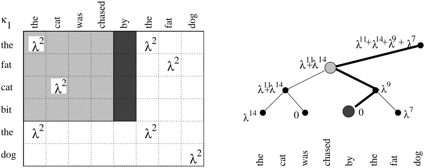
2Figure 5: The range-sum tree on the right, with a query path (emphasized edges) and an area of theκ1matrix corresponding to the query path (grey and black strips) on the left. Starting from the leaf, the values in nodes that are left children of their parents are added together.
will return the desired answer.
Figure 5 depicts the state of the range-sum tree when computing the valueκ2(5,6). The node 5 will contain value 0 as there are no subsequence co-occurrences within the strip(i,5),i<5. On the other hand, the key 4 will contain the valueλ11+λ14corresponding to the two co-occurrences within the (shaded) region(i,j),i<5,j∈[1,4], scaled with the dummy gaps: λ11=λ2λ6−3+8−2,λ14=
λ2λ6−1+8−1. The sum of weights in the shaded region is computed by adding the value 0 in node 5 corresponding to the empty black region, the value in node 4 corresponding to the grey region and skipping node 6 as 6>5.
The sparse dynamic programming algorithm is shown in Figure 6. The algorithm takes as input a set M1={M1(1), . . . ,M1(m)}of match lists
M1(i) = ((j1,κ1(i,j)),(j2,κ1(i,j)), . . .),
that have been created in a preprocessing step taking O(n+m+|Σ|+|M1|)time and space. This preprocessing involves creating for each character c∈Σa list I(c) ={j|tj=c}of indices in the string t that contain the character c. To create a match list M1(i)then involves copying the indices in I(si)to M1(i)and storing the corresponding valuesκ1(i,j) =λm−i+n−jλ2with the indices.
The main algorithm computes the kernel K(s,t) =κp(m,n)by incrementally working out match sets M2, . . . ,Mp, corresponding to subsequence lengths 2, . . . ,p.
The processing of subsequence length q entails making one pass through the match sets Mq−1(k) in increasing order of k. When constructing match list Mq(k) the algorithm traverses match list
Mq−1(k), and for each item(j,κ)in the list makes a range query RangeSum([1,l−1]) =∑i<k∑j<lκq−1(i,j), and, if the result is non-zero, inserts the item(l,RangeSum([1,l−1]))to the list Mq(k). After cre-ating each list Mq(k)the tree is updated with the contents of Mq−1(k).
Finally, the kernel value K(s,t) is computed by traversing the match lists Mp(k),1≤k≤m,
function K=SPARSE(M1,p,λ) for q=2 :(p−1)
RangeSum(1 :|t|) =0; % initially the ranges are empty for i=p : m
% compute the kappa values for the next level
Mq(i) ={};
for(jh,κh)∈Mq−1(i)
S=query(RangeSum,[1,jh−1]); % make range query if S>0
Mq(i) =Mq(i)∪(jh,S); end
end
% update the range with Mq−1(i) for(jh,κh)∈Mq−1(i)
update(RangeSum,(jh,κh)); end
end end
% compute the values for the final level
K=0;
for i=p :(m−1)
for(jh,κh)∈Mp−1(i); if jh<n
K=K+κhλi+jh; % rescale to remove the dummy gap end
end end
The queries and updates amount to O(log n)per item in the match list so the time complexity to process level q is O(|Mq|log n). Since we have|M1| ≥ |M2| ≥ · · · ≥ |Mp|, the total time complexity will be O(p|M1|log n). On random strings|M1| ≈ |s||t|/|Σ|. Hence, the sparse algorithm is likely to excel when log n/|Σ|is small, which we verify in the experiments presented in Section 4.
3.4 Variants and Implementation
The presented algorithm can be modified to compute many of the string kernel variants:
• A kernel only counting the number of co-occurrences of substrings is trivially obtained by settingλ=1. In practical implementation, one can remove the scaling/rescaling operations from the algorithm, thus reducing the constants hidden in the asymptotic time-complexity.
• Bounded-length subsequence kernels are straight-forward to obtain. For each subsequence length q≤l≤p, the sum of weights in the match lists, rescaled to remove the dummy gaps,
needs to be computed, as opposed for the length p only, as in the original algorithm. Thus, kernels of the form K(s,t) =∑qp=1wqKq(s,t),wq∈Rare easily obtained.
• Weighting by the number of gaps and the use of character specific gap penalties only require minor modifications to the algorithm (see below).
However, soft matching approaches (c.f Saunders et al., 2002), where most of the characters can be matched with each other with different costs (or utilities), are beyond this algorithm. This is because the efficiency of the algorithm relies on the match sets Mqto be sparse.
Weighting by the number of gaps. It is straightforward to modify the algorithm to penalize the number of gaps in the subsequence, instead of the total gap length. The kernel
κGap#(s,t) =
∑
u∈Σpφp
u(s)φup(t),withφup(s) =
∑
i:u=s(i)
λ∑j[ij+1−ij>1],u∈Σp,
can be computed via the recurrence
κq(k,l) = [si=tj]
∑
i<k−1,j<l−1
λ2κ
q−1(i,j) +
∑
i<k−1
λκq−1(i,l−1) +
∑
j<l−1λκq−1(k−1,j) +κq−1(k−1,l−1)
(8)
which again leads to the O(p|s||t|)time complexity. The first term takes into account co-occurrences where one gap is inserted to both the matched subsequences. The second and third term correspond to matches where a gap is inserted to occurrences in s only and t only, respectively. The last term takes into account matches where no gap is inserted to either s or t.
The sparse dynamic programming algorithm can be made to compute this recurrence effi-ciently by a simple modification: The range sum tree updates need to be lagged by one iteration so that, when creating the match list Mq(k), the tree will not yet contain the values in the match list
Mq−1(k−1); these values will be added to the tree after handling the match list Mq(k). By such an arrangement, the recurrence can be computed as
κq(k,l) = [si=tj]
λ2·Rangesum([1,l−2])+λ·Rangesum([l−1,l−1])+λr(j)+κ
q−1(k−1,l−1)
where the values r(j) =∑j<l−1κq−1(k−1,j) are incrementally computed while processing the match list Mq−1(k−1). The algorithm’s time complexity O(p|M|log n)will not change.
Character-specific gap and match weights. Another variant is to let the gap penalty depend on the character that was skipped, so that we have a set of penalties{λa|a∈Σ}. To implement this we need to precompute a vectorΛs= (λs,k)|ks=|1, λs,k=λs1× · · · ×λsk and an analogous vectorΛt
for string t. In the algorithm, when storing the item κq−1(i,j) in the range sum tree, it is first scaled byλs,m/λs,i·λt,n/λt,j to introduce a dummy gaps s(i+1 : m)and t(j+1 : n)with character specific weighting. As with uniform gap weights, when computing the final level, rescaling by
λs,k/λs,m·λt,l/λt,nis needed to recover the valueκp(k,l).
The approach can easily extended to handle different weights for matches and gaps, as suggested by Cancedda et al., (2003). This only requires performing a scaling
κq(k,l) =
γsk
λsk
γtl
λtl
RangeSum([1,l−1]),
whereγaandλaare the match and gap decays for letter a, respectively, to reflect the fact that skwas matched to tlrather than skipped over.
Implementation. The algorithm described above has been implemented in MATLAB 7.0. The code has been heavily tweaked to ensure that the benefits suggested by theoretical analysis can also be realized in practise. The major tweaks include
• Range sum tree storage. In our MATLAB implementation, the range sum tree is implicitly stored in a weight vector w storing the sum of the left subtree of each node 1≤j≤n. To speed
up computations we also precompute in separate tables the nodes that need to be visited when querying or updating the range sum tree. For example, in the situation depicted in Figure (5) the precomputed query path for will contain the nodes 4 and 5. The corresponding update
path will contain the nodes 6 and 8.
• Avoiding numerical underflow. The algorithm in Figure 6 stores the items in the form
λm−i+n−jκ
q−1(i,j) and rescales them when computing the level p. This approach suffers from the potential of numerical underflow when handling long strings. In order to avoid that, we divide the index plane into rectangles of height and width sufficiently small (depending on the valueλ) such that within a rectangle[x0,x00]×[y0,y00]the values are stored in the form
λx00+y00−i−j. The handling of the boundaries of the rectangles causes a small additive overhead to the time complexity. The same technique can be used with the above discussed variants as well.
The implementation of the sparse dynamic programming algorithm is available via WWW from the home page of Juho Rousu: htt p ://www.cs.helsinki.f i/juho.rousu.
4. Empirical Evaluation
We compared the time consumption of the following gapped string kernel algorithms, all imple-mented in MATLAB:
2 4 8
16 3264 128
25651210242048 32
64 128 256 512 1024 2048 4096 8192 0.01 0.1 1 10 100 1000 10000
alphabet size |A|
Time consumption of SPARSE on random strings
string length |s|,|t|
time (s)
2 4 8 16 32 64 128 256 512 1024 2048 32 64
128 256 5121024
2048 40968192 10%
50% 100% 500% 1000%
alphabet size |A|
Relative time consumption: time(SPARSE)/time(DYNPROG)
string length |s|,|t|
relative time consumption
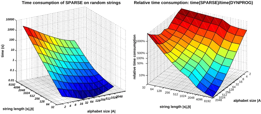
Figure 7: The time consumption of SPARSE in seconds (left) and relative time consumption of SPARSE relative to the time consumption of DYNPROG (right). The subsequence length p=10 was used. Note the logarithmic scale on all axes.
DYNPROG. The full dynamic programming approach of Section 3.2.
TRIE. The Trie-based computation approach of Section 3.1.
Note that, differently from TRIE, DYNPROGand SPARSEplace no hard restriction on the gap length
but softly penalize the increase in gap length. We used three data sets for comparing the algorithms.
• Randomly generated strings, with varying length and alphabet sizes.
• 1000 random English news article pairs from the Reuters-21578 corpus, represented as se-quences of syllables. The size of the syllable alphabet was 3769.
• 1000 random document pairs from the Chinese part of the Reuter’s multilingual RCV-2 cor-pus. The size of the alphabet was 3142.
The tests were run on a 3GHZ Pentium 4 processor with 1.5GB main memory.
4.1 Results on Random Strings
In our first test we tested the time-consumption of the algorithm SPARSE as a function of string length and alphabet size. Figure 7 depicts the results. On the left the algorithms absolute time consumption is shown. The inverse dependency of the time-consumption on the alphabet size is clearly visible. Also, the larger the alphabet, the slower the time-consumption increases when the string length is increased.
2 32
128 512 2048 0
2 4 6 8 10% 100% 1000% 10000%
alphabet size |A|
Relative time consumption: time(TRIE)/time(SPARSE)
gap length
relative time consumption
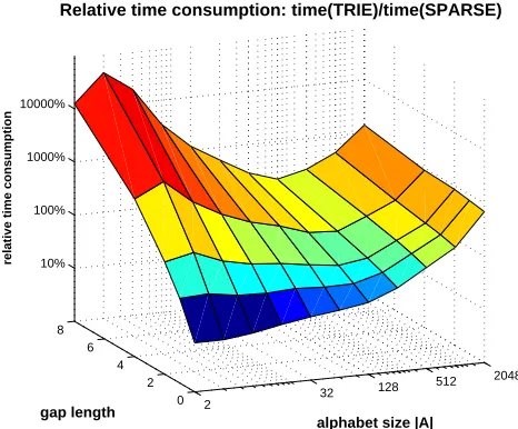
Figure 8: The relative time consumption time(TRIE)/time(SPARSE) of the algorithms, as a function of alphabet size and gap length. The subsequence length p=10 and string length|s|,|t|= 512 was used. Note the logarithmic scale.
SPARSE. With long strings and large alphabets the roles reverse: on strings longer than 1024 letters
and alphabet sizes over 256, the SPARSEcan be an order of magnitude faster then DYNPROG.
In our second test we compare the speed of TRIEalgorithm to the SPARSEalgorithm. Figure 8 depicts the relative time consumption as a function of alphabet size and gap length. Subsequence length of 10 and string length of 512 were used. Since SPARSE does not place any restriction to
the gap length, in the comparison only the time taken by TRIEactually varied when the maximum number of gaps was varied.
The figure shows that TRIEalgorithm gets very significantly slower than SPARSEwhen more gaps are allowed especially so on small alphabets. TRIE is faster than SPARSE only when the number of gaps is restricted to 2 or below. On very large alphabets even disallowing gaps does not bring TRIEbelow the time consumption of SPARSE.
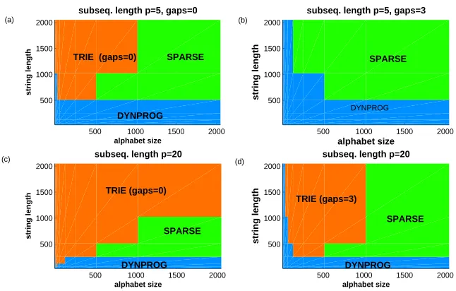
The fastest algorithm as a function of string length and alphabet size is depicted in Figure 9, with different settings for the subsequence length (p) and the maximum number of gaps allowed in the TRIEalgorithm. DYNPROG is the fastest method on short strings independent on the alphabet
size and the subsequence length (a-d). If no gaps are allowed, TRIE is competitive on small to medium-size alphabets and long strings (a). When the subsequence length is increased, TRIE is faster than SPARSE even on large alphabets (c). The situation changes when gaps are allowed
500 1000 1500 2000 500
1000 1500 2000
alphabet size
subseq. length p=5, gaps=0
string length
500 1000 1500 2000 500
1000 1500 2000
subseq. length p=5, gaps=3
alphabet size
string length
500 1000 1500 2000 500
1000 1500 2000
subseq. length p=20
alphabet size
string length
500 1000 1500 2000 500
1000 1500 2000
alphabet size
subseq. length p=20
string length
SPARSE TRIE (gaps=0)
DYNPROG
SPARSE
DYNPROG
TRIE (gaps=0)
SPARSE
DYNPROG
TRIE (gaps=3)
SPARSE
DYNPROG
(a) (b)
(c) (d)
Figure 9: The fastest algorithm as a function of string length and alphabet size, with different sub-sequence lengths (p) and upper bounds for the number of gaps in the TRIEalgorithm.
4.2 Results on Reuter’s News Articles
Our second set of experiments tests the speed of kernel computation on two Reuter’s newswire article data sets, English articles from Reuters-21578 corpus represented as sequences of syllables and Chinese articles from the multilingual RCV-2 corpus.
We computed the gap-weighted string kernel using DYNPROG and SPARSEfor 1000 random
document pairs, varying the subsequence lengths in the range 5-20. In our preliminary experiments, TRIEwas significantly slower than both of the dynamic programming approaches on these data sets. Hence, we omitted that algorithm from the comparison.
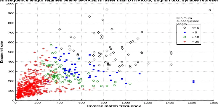
The results on the English news articles are summarized in Figure 10. In the figure each docu-ment pair is plotted to the location corresponding to the (geometric) mean length of the docudocu-ments (x-axis) and the inverse of the match frequency|s||t|/|M|(y-axis), which also can be thought as the effective alphabet size: if the syllables were independently randomly drawn from alphabet of size|Σ|=|s||t|/|M|, the expected size of the match set would be|M|. Note that, due to the skewed distribution of syllables in the documents this number is usually significantly lower than the size of the syllable alphabet.
The marker type corresponds to the minimum subsequence length p required to make SPARSE
run faster than DYNPROG on that document pair. Document pairs marked with ’+’ require p>
0 200 400 600 800 1000 1200 1400 1600 1800 0
100 200 300 400 500 600 700 800 900 1000
Inverse match frequency
Document size
Subsequence length regimes where SPARSE is faster than DYNPROG, English text, syllable representation
<= 5 > 5 > 10 > 20 Minimum subsequence length
Figure 10: Regimes of subsequence length p, document size (x-axis) and inverse frequency of matching letters (y-axis), where SPARSEis faster than DYNPROGon English syllable-represented news articles. Document pairs marked with ’+’ require p>20, circles re-quire 11≤p≤20, boxes require 6≤p≤10, and for diamonds p=5 is sufficient.
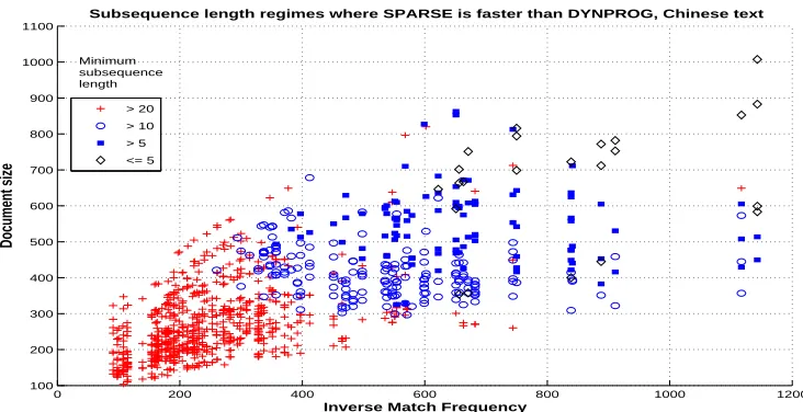
The results on Chinese news are summarized in Figure 11. The behaviour of the algorithms can be seen to be essentially the same as on the syllable converted English text: long documents and a sparse match matrix favour SPARSE.
5. Discussion and Open Problems
Based on the presented experiments, the full dynamic programming approach is the fastest method on short strings. On longer strings, the best algorithm depends on other parameters: if the alphabet is large the new sparse dynamic programming approach is the fastest method, if the alphabet is small DYNPROG is the best method. On medium-sized alphabets, the trie-based approach is competitive
if the number of gaps can be strongly restricted.
The observed relative performance can be explained as follows. When the alphabet size is small, allowing more gaps rapidly expands the number of partially matching subsequences. Since TRIEexplicitly keeps track of them, its time-consumption increases. SPARSEalso suffers on small
alphabets. However, it can never be worse than DYNPROGby more than a log n factor. On large alphabets, TRIEhas an overhead of keeping track of all subtrees that may or may not need to be expanded. The improving performance of TRIEby increasing subsequence length is also easy to
explain: the trie becomes the sparser the deeper the search level. Thus deepening the search is relatively cheap.
0 200 400 600 800 1000 1200 100
200 300 400 500 600 700 800 900 1000 1100
Inverse Match Frequency
Document size
Subsequence length regimes where SPARSE is faster than DYNPROG, Chinese text
> 20 > 10 > 5 <= 5 Minimum subsequence length
Figure 11: Regimes of subsequence length p, document size (x-axis) and inverse frequency of matching letters (y-axis), where SPARSEis faster than DYNPROG on Chinese news ar-ticles. Document pairs marked with ’+’ require p>20, circles require 11≤ p≤20, boxes require 6≤p≤10, and for diamonds p=5 is sufficient.
per query (Agarwal and Erickson, 1999), even when taking advantage of the fact that the points are situated on an integer grid (Overmars, 1988, Alstrup et al., 2000). On the other hand the best lower bounds are of orderΩ(log log n)per query (Chazelle, 1995).
There are amortized O(α(n))time range query methods, whereα(n)is the inverse Ackermann’s function, but they require O(|s||t|)(Chazelle and Rosenberg, 1989) or O(|M|2)preprocessing (Poon, 2003)—which would lead to O(p|s||t|)and O(p|M|2)total time complexity in our case, if applied in a straightforward manner. But, could we get O(p|M|α(|M|)+|s||t|)complexity by taking advantage of the fact that the match sets satisfy M1⊃M2⊃ · · · ⊃Mp? Moreover, each match set Ml is highly structured: for each l≤i≤ |s| we make the the range query sequence [1,j1]⊂[1,j2]⊂ · · · ⊂ [1,jr], where si =tjh,l< jh≤ |t|. In addition, for i and i
0 that satisfy si =s
i0 exactly the same
query sequence is made. However, taking advantage of this appears to be non-trivial. For example, maintaining a separate range-query index for each character would result in O(p|M||Σ|)≈O(p|s||t|) time complexity.
6. Conclusions
We presented a sparse dynamic programming algorithm that efficiently computes the gap-weighted string kernels. The algorithm is easily adaptable to different string kernel variants, including fixed-length and bounded-fixed-length subsequence kernels and different gap penalization schemes, includ-ing penalization by total length of the gaps and number of the gaps as well as character specific gap/match penalization.
to be useful in document classification tasks (Saunders et al., 2002, Cancedda et al., 2003). As the algorithm scales well to long documents when the alphabet is large, it could find use in classification of longer documents than the relatively short news stories, for instance, full-length research articles.
Acknowledgments
We thank Yaoyong Li and Craig Saunders for the help preparing the data sets. The work by Juho Rousu has been supported by the EU/Marie Curie Fellowship grant HPMF-CT-2002-02110. This work was supported in part by the IST Programme of the European Community, under the PASCAL Network of Excellence, IST-2002-506778. This publication only reflects the authors’ views.
References
P. Agarwal and J. Erickson. Geometric range searching and its relatives. Contemporary Mathematics 23:
Advances in Discrete and Computational Geometry, pages 1–56, 1999.
S. Alstrup, G.S. Brodal, T. Rauhe. New Data Structures for Orthogonal Range Searching. In Proceedings
of 41st Annual Symposium on Foundations of Computer Science, pages 198-207, 2000.
B. S. Baker and R. Giancarlo. Longest common subsequence from fragments via sparse dynamic program-ming. In Proceedings of Sixth Annual European Symposium on Algorithms, pages 79–90, 1998.
M. de Berg, M. van Kreveld, M. Overmars, and O. Schwarzkopf. Computational Geometry – Algorithms
and Applications. Springer-Verlag, Berlin, 1997.
N. Cancedda, E. Gaussier, C. Goutte, J-M. Renders. Word-Sequence Kernels. Journal of Machine Learning
Research 3:1059–1082, 2003.
B. Chazelle. Lower bounds for off-line range searching. In Proceedings of 27th Annual ACM Symposium
on Theory of Computing, pages 733–740, 1995.
B. Chazelle and B. Rosenberg. Computing partial sums in multidimensional arrays. In Proceedings of 5th
Annual Symposium on Computational Geometry, pages 131–139, 1989.
N. Cristianini and J. Shawe-Taylor. An introduction to Support Vector Machines. Cambridge University Press, 2000.
D. Eppstein. Efficient algorithms for sequence analysis with concave and convex gap costs. Ph.D. thesis, Columbia University, 1989.
D. Eppstein, Z. Galil, R. Giancarlo, and G. F. Italiano. Sparse dynamic programming I: linear cost functions.
Journal of the ACM 39, 3:519–545, 1992.
D. Haussler. Convolution kernels on discrete structures. Technical report, University of California, Santa Cruz, 1999.
T. Joachims. Text Categorization with Support Vector Machines: Learning with Many Relevant Features. In Proceedings of Tenth European Conference on Machine Learning, pages 137–142, 1999.
C. Leslie, E. Eskin and W. Stafford Noble. The spectrum kernel: a string kernel for SVM protein classifica-tion. In Proceedings of Pacific Symposium on Biocomputing 7, pages 566–575, 2002.
C. Leslie and R. Kuang. Fast Kernels for Inexact String Matching. In Proceedings of 16th Conference
on Computational Learning Theory and 7th Kernel Workshop, COLT/Kernel’2003. Lecture Notes in Computer Science 2777:114 - 128, 2003.
H. Lodhi, C. Saunders, J. Shawe-Taylor, N. Cristianini and C. Watkins. Text Classification using String Kernels. Journal of Machine Learning Research 2:419–444, 2002.
V. M¨akinen. Parameterized Approximate String Matching and Local-Similarity-Based Point-Pattern Match-ing. Report A-2003-6. Department of Computer Science, University of Helsinki, 2003.
M. Overmars. Efficient data structures for range searching on a grid. Journal of Algorithms 9:254–275, 1988.
C. Poon. Dynamic orthogonal range queries in OLAP. Theoretical Computer Science 296(3):487–510, 2003.
G. Salton, A. Wong and C.S. Yang. A Vector Space Model for Automatic Indexing. Communications of the
ACM 18(11):613–620, 1973.
C. Saunders, H. Tschach and J. Shawe-Taylor. Syllables and other String Kernel Extensions. In Proceedings
of 19th International Conference on Machine Learning, pages 530–537, 2002.
J. Shawe-Taylor and N. Cristianini. Kernel Methods for Pattern Analysis. Cambridge University Press, 2004.
V. Vapnik. The Nature of Statistical Learning Theory. Springer Verlag, 1995.
S. Vishwanathan and A. Smola. Fast Kernels for String and Tree Matching. Advances in Neural Information
Processing Systems 15, pages 569–576, 2003,
C. Watkins. Dynamic alignment kernels. In A.J. Smola, P. Bartlett, B. Sch¨olkopf and D. Schuurmans, eds.,