A Linear Difference Scheme for Dissipative Symmetric Regularized Long Wave Equations with Damping Term

Boundary Value Problems

Volume 2010, Article ID 781750,16pages doi:10.1155/2010/781750

Research Article

A Linear Difference Scheme for Dissipative

Symmetric Regularized Long Wave Equations with

Damping Term

Jinsong Hu,

_{Youcai Xu,}

_{and Bing Hu}

1_{School of Mathematics and Computer Engineering, Xihua University, Chengdu 610039, China}

2_{School of Mathematics, Sichuan University, Chengdu 610064, China}

Correspondence should be addressed to Youcai Xu,xyc@scu.edu.cn

Received 24 August 2010; Accepted 14 November 2010

Academic Editor: V. Shakhmurov

Copyrightq2010 Jinsong Hu et al. This is an open access article distributed under the Creative Commons Attribution License, which permits unrestricted use, distribution, and reproduction in any medium, provided the original work is properly cited.

We study the initial-boundary problem of dissipative symmetric regularized long wave equations with damping term by finite difference method. A linear three-level implicit finite difference scheme is designed. Existence and uniqueness of numerical solutions are derived. It is proved that the finite difference scheme is of second-order convergence and unconditionally stable by the discrete energy method. Numerical simulations verify that the method is accurate and efficient.

1. Introduction

A symmetric version of regularized long wave equationSRLWE,

utρxuux−uxxt0,

ρtux0,

1.1

has been proposed to model the propagation of weakly nonlinear ion acoustic and space charge waves1 . The sec2_{solitary wave solutions are}

ux, t 3

v2₋₁ v sec

21 2

v2₋₁

v2 x−vt,

ρx, t 3

v2₋₁ v2 sec

21 2

v2₋₁

v2 x−vt.

The four invariants and some numerical results have been obtained in 1 , where vis the velocity,v2_{>1. Obviously, eliminatingρfrom1.1, we get a class of SRLWE:}

utt−uxx

1 2

u2

xt−uxxtt0. 1.3

Equation1.3is explicitly symmetric in thex andt derivatives and is very similar to the regularized long wave equation that describes shallow water waves and plasma drift waves

2, 3 . The SRLW equation also arises in many other areas of mathematical physics 4–6 . Numerical investigation indicates that interactions of solitary waves are inelastic7 ; thus, the solitary wave of the SRLWE is not a solution. Research on the wellposedness for its solution and numerical methods has aroused more and more interest. In8 , Guo studied the existence, uniqueness, and regularity of the numerical solutions for the periodic initial value problem of generalized SRLW by the spectral method. In9 , Zheng et al. presented a Fourier pseudospectral method with a restraint operator for the SRLWEs and proved its stability and obtained the optimum error estimates. There are other methods such as pseudospectral method, finite difference method for the initial-boundary value problem of SRLWEssee9–

15 .

In applications, the viscous damping effect is inevitable, and it plays the same important role as the dispersive effect. Therefore, it is more significant to study the dissipative symmetric regularized long wave equations with the damping term

utρx−υuxxuux−uxxt0, 1.4

ρtuxγρ0, 1.5

whereυ, γare positive constants,υ >0 is the dissipative coefficient, andγ >0 is the damping coefficient. Equations 1.4-1.5are a reasonable model to render essential phenomena of nonlinear ion acoustic wave motion when dissipation is considered. Existence, uniqueness, and wellposedness of global solutions to 1.4-1.5 are presented see 16–20 . But it is difficult to find the analytical solution to 1.4-1.5, which makes numerical solution important.

To authors’ knowledge, the finite difference method to dissipative SRLWEs with

damping term1.4-1.5has not been studied till now. In this paper, we propose linear three level implicit finite difference scheme for1.4-1.5with

ux,0 u0x, ρx,0 ρ0x, x∈xL, xR , 1.6

and the boundary conditions

uxL, t uxR, t 0, ρxL, t ρxR, t 0, t∈0, T . 1.7

We show that this difference scheme is uniquely solvable, convergent, and stable in both theoretical and numerical senses.

Lemma 1.1. Suppose thatu0∈H1_{,ρ0∈L2, the solution of1.4–1.7satisfiesu}

L2 ≤C,uxL2 ≤

Proof. Let

Et u2L2ux

2

L2ρ

2

L2

xR

xL

u2dx xR

xL

ux2dx

xR

xL

ρ2dx, t∈0, T . 1.8

Multiplying1.4byuand integrating overxL, xR , we have

xR

xL

uutuρx−υuuxxu2ux−uuxxt

dx0. 1.9

According to

_xR

xL

uutdx

1 2

d dt

_xR

xL u2dx,

xR

xL

uρxdxuρ|xxRL− xR

xL

ρdu− xR

xL

uxρdx,

− _xR

xL

uuxxdx−uux|xxRL _xR

xL

uxdu

_xR

xL

ux2dx,

xR

xL

u2uxdx 1

3u 3_|xR

xL 0,

− _xR

xL

uuxxtdx−uuxt|xxRL _xR

xL

uxtdu

1 2

d dt

_xR

xL

ux2dx,

1.10

we get

d dt

xR

xL

u2u2x

dx−2

xR

xL

uxρdx2υ

xR

xL

ux2dx0, 1.11

Then, multiplying1.5byρand integrating overxL, xR , we have

xR

xL

ρρtρuxγρ2

dx0. 1.12

By

xR

xL

ρρtdx

1 2

d dt

xR

xL

ρ2dx, 1.13

we get

d dt

_xR

xL

ρ2dx2 _xR

xL

uxρdx2γ

_xR

xL

Adding1.14to1.11, we obtain

d dt

xR

xL

u2u2xρ2

dx−2υ xR

xL

ux2dx−2γ

xR

xL

ρ2dx≤0. 1.15

SoEtis decreasing with respect tot, which implies thatEt u2

L2ux

2

L2ρ

2

L2≤E0,

t ∈ 0, T . Then, it indicates that uL2 ≤ C,uxL2 ≤ C, andρL2 ≤ C. It is followed from

Sobolev inequality thatuL∞ ≤C.

2. Finite Difference Scheme and Its Error Estimation

Lethandτbe the uniform step size in the spatial and temporal direction, respectively. Denote xj xLjhj 0,1,2, . . . , J,tn nτn 0,1,2, . . . , N,N T/τ ,un_j ≈ uxj, tn,ρn_j ≈

ρxj, tn, andZ0_h{u uj|u0uJ 0, j0,1,2, . . . , J}. We define the difference operators

as follows:

un

j

x

un_j1−un_j

h ,

un

j

x

un_j −un_j−1

h ,

un

j

x

un_j1−un_j−1

2h ,

un

j

t

un_j1−un_j−1

2τ ,

unj

un1

j unj−1

2 , u

n_{, v}n_hJ−1 j0

un_jv_jn, un2un, un, un_∞ max 0≤j≤J−1

un_j.

2.1

Then, the average three-implicit finite difference scheme for the solution of1.4–1.7is as follow:

un_j

t−

un_j

xxt

ρ_jn

x−υ

unj

xx

1 3

un_junj

x

un_junj

x

0, 2.2

ρ_jn

t

un_j

xγρ n

j 0, 2.3

u0_j u0xj

, ρ0_j ρ0xj

, 0≤j≤J, 2.4

un

0 unJ 0, ρn0 ρnJ 0, 1≤n≤N. 2.5

Lemma 2.1. Summation by parts follows [12,21] that for any two discrete functionsu, v∈Z0

h

uj

x, vj

−uj,

vj

x

, vj,

uj

xx

−vj

x,

uj

x

Lemma 2.2discrete Sobolev’s inequality 12,21 . There exist two constantsC1 andC2 such that

un_∞≤C1unC2unx. 2.7

Lemma 2.3discrete Gronwall inequality12,21 . Suppose thatwk,ρkare nonnegative functions and ρkis nondecreasing. IfC >0and

wk≤ρk Cτ

k−1

l0

wl. 2.8

Thenwk≤ρkeCτk_.

Theorem 2.4. Ifu0∈H1_{,ρ0∈L2, then the solution of 2.2–2.5satisfies}

un ≤C, unx ≤C, ρn≤C, un∞≤C n1,2, . . . , N. 2.9

Proof. Taking an inner product of 2.2 with 2unj i.e., ujn1 unj−1 and considering the

boundary condition2.5andLemma 2.1, we obtain

1 2τ

un12−un−12

1

2τ

unx1

2

−unx−1

2

ρn_j

x,2u n j

−υunj

xx,2u n j

P,2unj

0,

2.10

whereP 1/3un_junjx unju n

jx . Since

ρn

j

x,2u n j

−ρn j,2

unj

x

,

unj

xx,2u n j

−2unx

2 ,

P,2unj

2

3h

J−1

j0

unj

unj

x

unjunj

x

unj

1

12

J−1

j0

u_jnun_j11un_j−₁1−un_j−11−un_j−−₁1un_j1un_j11un_j−₁1−u_jn₋₁un_j−11un_j−−₁1

×un1

j unj−1

1

12

J−1

j0

un j unj1

un1

j1 unj−11

un1

j unj−1

−1 12

J−1

j0

un_j un_j−1un_j1u_jn−1un_j−11un_j−−₁10,

we obtain

1 2τ

un12−un−12

1

2τ

unx1

2

−unx−1

2

−ρjn,2

unj

x

2υunx

2

0. 2.12

Taking an inner product of2.3with 2ρn_j i.e., ρn1

j ρnj−1, we obtain

1 2τ

ρn12_−ρn−12

un j

x,2ρ n j

2γρn_j2 0. 2.13

Adding2.12to2.13, we have

un12−un−12unx1

2

−unx−1

2

ρn12−ρn−12

2τρn j,2

unj

x

−un

j

x,2ρ n j

−4υτunx

2₋

4γτρn_j2.

2.14

Since

ρnj,2

unj

x

ρnj,

unj1

x

unj−1

x

≤ρn21 2

unx1

2

unx−1

2 ,

−un_j

x,2ρ n j

−un_j

x, ρ n1

j ρjn−1

≤ unx2

1 2

ρn12ρn−12

.

2.15

Equation2.14can be changed to

un12−un−12unx1

2

−unx−1

2

ρn12−ρn−12

≤Cτunx1

2

unx2unx−1

2

ρn12ρn2ρn−12

.

2.16

LetAn_un12_un2_un1

x 2unx2ρn12ρn2, and2.16is changed to

An−An−1≤CτAnAn−1. 2.17

Ifτis sufficiently small which satisfies 1−Cτ >0, then

An−An−1≤CτAn−1. 2.18

Summing up2.18from 1 ton, we have

An_≤A0_Cτn−1

l0

FromLemma 2.3, we obtainAn _{≤ C, which implies that,u}n _{≤ C,u}n

x ≤ C, andρn ≤ C.

ByLemma 2.2, we obtainun ∞≤C.

Theorem 2.5. Assume thatu0_∈H2_,ρ0_∈H1_{, the solution of difference scheme2.2–2.5satisfies: ρ}n

x≤C, unxx ≤C, unx∞≤C, ρn∞≤C n1,2, . . . , N. 2.20

Proof. Differentiating backward2.2–2.5with respect tox, we obtain

un_j

xt−

un_j

xxxt

ρn_j

xx−υ

unj

xxx

1 3

un_junj

x

un_junj

x

x 0, 2.21

ρn_j

xt

un_j

xxγ

ρn_j

x0, 2.22

u0_j

xu0,x

xj

, ρ0_j

xρ0,x

xj

, 0≤j≤J, 2.23

un_0xun_J

x0,

ρn_0xρn_J

x0, 0≤n≤N. 2.24

Computing the inner product of2.21with 2unx i.e., uxn1unx−1and considering2.24and

Lemma 2.1, we obtain

1 2τ

unx1

2

−unx−1

2

1

2τ

unxx1

2

−unxx−1

2

ρn_xx,2unx

−υun_xxx,2unx

R,2unx

0,

2.25

whereR 1/3un_junjx unju n

jx x. It follows fromTheorem 2.4that

un_j≤C j 0,1,2, . . . , J. 2.26

By the Schwarz inequality andLemma 2.1, we get

R,2unx

2

3

un_junj

x

un_junj

x

x, u n x −2 3

un_junj

x

un_junj

x, u n xx

−2 3h

J−1

j0

unj

unj

x

unjunj

x

unj

xx

≤ 2 3Ch

J−1

j0 unj

x

·unj

xx

≤Cunx

2 unxx

2

≤Cunx1

2

unx−1

2

unxx1

2

unxx−1

2 .

Noting that

ρn_xx,2unx

−2unxx, ρxn

−ρnx, unxx1unx−x1

≤ρxn2

1 2

unxx1

2

unxx−1

2 ,

unxxx,2unx

−2unxx

2 ,

2.28

it follows from2.25that

unx1

2

−unx−1

2

unxx1

2

−unxx−1

2

≤ −4υτunxx

2

Cτunx1

2

unx−1

2

unxx1

2

unxx−1

2

ρnx

2 .

2.29

Computing the inner product of2.22with 2ρn_xi.e.,ρn1

x ρnx−1and considering2.24and

Lemma 2.1, we obtain

1 2τ

ρnx1

2

−ρxn−1

2

un_xx, ρn_x2γρn_x20. 2.30

Since

un_xx,2ρn_xun_xx, ρnx1ρnx−1

≤ unxx2

1 2

ρxn1

2

ρnx−1

2

, 2.31

then2.30is changed to

ρxn1−ρxn−1≤ −4γτρnx

2 Cτ

unxx2ρxn1

2

ρnx−1

2

. 2.32

Adding2.29to2.32, we have

unx1

2

−unx−1

2

unxx1

2

−unxx−1

2

ρnx1

2

−ρxn−1

2

≤ −4υτunxx

2₋

4γτρn_x2

Cτun1

x

2

un−1

x

2

un

xx2unxx1

2

un−1

xx

2

ρn1

x

2

ρn x

2 ρn−1

x

2

≤Cτunx1

2

unx−1

2

unxx2unxx1

2

unxx−1

2

ρnx1

2

ρxn

2 ρnx−1

2 .

2.33

LetingBn_un1

x 2unx2uxxn12unxx2ρxn12ρnx2, we obtainBn−Bn−1≤CτBn

Bn−1_{. Choosing suitableτwhich is small enough to satisfy 1−Cτ >0, we get}

Summing up2.34from 1 ton, we have

Bn≤B0Cτ

n−1

l0

Bl. 2.35

By Lemma 2.3, we get Bn _{≤ C, which implies that ρ}n

x ≤ C,unxx ≤ C. It follows from

Theorem 2.4andLemma 2.2thatun

x∞≤C,ρn∞≤C.

3. Solvability

Theorem 3.1. The solutionun_{of2.2–2.5is unique.}

Proof. Using the mathematical induction, clearly,u0_,ρ0 _{are uniquely determined by initial} conditions2.4. then select appropriate second-order methodssuch as the C-N Schemes and calculate u1 _{and ρ}1 _{i.e. u}0_{, ρ}0_{, and u}1_{, ρ}1 _{are uniquely determined. Assume that} u0_{, u}1_{, . . . , u}n_andρ0_{, ρ}1_{, . . . , ρ}n_{are the only solution, now consideru}n1_andρn1_in2.2and

2.3:

1 2τu

n1

j −

1 2τ

un_j1

xx−

υ 2

un_j1

xx

1 6

un_jun_j1

x

un_jun_j1

x

0, 3.1

1 2τρ

n1

j

γ 2ρ

n1

j 0. 3.2

Taking an inner product of3.1withun1_{, we have}

1 2τ

un12 1 2τ

unx1

2

υ

2 unx1

2

1

6h

J−1

j0

un_jun_j1

x

un_jun_j1

x

un_j10. 3.3

Since

1 6h

J−1

j0

un_jun_j1

x

un_jun_j1

x

un_j1

1

12

J−1

j0

u_jnun_j11−u_jn₋₁1un_j1un_j11−un_j−1un_j−11un_j1

1

12

J−1

j0

un_jun_j1un_j11u_jn₁un_j1u_jn₁1− 1 12

J−1

j0

un_j−1u_jn₋₁1un_j1un_jun_j−11un_j10,

3.4

then it holds

1 2τ

un12

1 2τ

υ 2

unx1

2

Taking an inner product of3.2withρn1_{and adding to3.5, we have}

1 2τ

un12

1 2τ

υ 2

unx1

2

1 2τ

γ 2

ρn120, 3.6

which implies that3.1-3.2have only zero solution. So the solutionun1

j andρnj1of2.2–

2.5is unique.

4. Convergence and Stability

Let vx, t and ∅x, t be the solution of problem 1.4–1.7; that is, v_jn uxj, tn, ∅n_j

ρxj, tn, then the truncation of the difference scheme2.2–2.5is

rjn

vnj

t−

vnj

xxt

∅n

j

x−υ

vnj

xx

1 3

vnj

vnj

x

vjnvnj

x

, 4.1

sn_j ∅n_j

t

vn_j

xγ∅ n

j. 4.2

Making use of Taylor expansion, it holds|r_jn||sn_j|Oτ2h2ifh, τ → 0.

Theorem 4.1. Assume thatu0 ∈ H1_{,ρ0 ∈L2, then the solutionu}n_andρn_{in the senses of norms} · ∞and · L2, respectively, to the difference scheme2.2–2.5converges to the solution of problem 1.4–1.7and the order of convergence isOτ2_h2_.

Proof. Subtracting2.2from4.1subtracting2.3from4.2, and lettingen_j v_jn−un_j,ηn_j

∅n

j −ρnj, we have

r_jnen_j

t−

en_j

xxt

η_jn

x−υ

enj

xxQ, 4.3

sn_j η_jn

t

e_jn

xγη n

j, 4.4

where

Q 1 3

v_jnvnj

x−u n j

unj

x

1

3

v_jnvnj

x−

un_junj

x

. 4.5

Computing the inner product of4.3with 2en, we get

en12−en−12exn1

2

−enx−1

2

−4υτenx

2

2τr_jn,2enj

−ηn_j

x,2e n j

−Q,2enj

.

According to

−Q,2enj

−2 3h

J−1

j0

vn_jvnj

x−u n j

unj

x

enj −

2 3h

J−1

j0

vn_jvnj

x−

un_junj

x

enj

−2 3h

J−1

j0

vn_jenj

xe n j

unj

x

enj

2 3h

J−1

j0

vn_jvnj −unju n j

enj

x

−2 3h

J−1

j0

vn_jenj

xe n j

unj

x

enj

2 3h

J−1

j0

en_jvnj unje n j

enj

x,

4.7

it follow fromLemma 1.1, Theorems2.4, and2.5that

vn_j≤C, vnj≤C,

unj

x

≤C, un_j≤C j0,1,2, . . . , J. 4.8

By the Schwarz inequality, we obtain

−Q,2en≤ 2 3Ch

J−1

j0

enj

x en j ·enj

2 3Ch

J−1

j0 _en

jenj

·enj

x

≤Cenx

2

en2en2

≤Cen12en2en−12enx1

2

enx−1

2 .

4.9

Since

r_jn,2enj

r_jn, en_j1e_jn−1≤ rn21 2

en12en−12

,

−ηn_j

x,2e n j

ηn_j,2enj

x

≤ηn21 2

exn1

2

enx−1

2 ,

4.10

it follows from4.9–4.10and4.6that

en12−en−12enx1

2

−enx−1

2

≤2τrnCτen12en2en−12enx1

2

enx−1

2

η2

.

Computing the inner product of4.4with 2ηn, we obtain

ηn12−ηn−122τsn_j,2η_jn−2τen_j

x,2η n j

−2γτηn2

≤Cτηn12ηn−12enx2

2τsn2.

4.12

Adding4.12to4.11, we have

en12−en−12enx1

2

−exn−1

2

ηn12 ηn−12

≤2τrn22τsn2Cτen12en2en−12enx1

2

en−1

x

2

en

x2ηn1

2

ηn2 ηn−12

.

4.13

Leting

Dn_en2_en12_en

x2enx1

2

ηn2

ηn12_{, 4.14}

we get

Dn−Dn−1≤2τrn22τsn2CτDn1Dn. 4.15

Ifτis sufficiently small which satisfies 1−Cτ >0, then

Dn_−Dn−1_≤CτDn−1_Cτrn2_Cτsn2_{. 4.16}

Summing up4.16from 1 ton, we have

Dn≤D0Cτ

n

l1

rl2Cτ

n

l1

sl2Cτ

n−1

l0

Dl. 4.17

Select appropriate second-order methodssuch as the C-N Schemes, and calculateu1 _and ρ1_{, which satisfies}

Noticing that

τ

n

l1

rl2_≤nτmax

1≤l≤n

rl2_≤T·Oτ2_h22_,

τ

n

l1

sl2≤nτmax 1≤l≤n

sl2≤T·Oτ2h22,

4.19

we then have

Dn≤Oτ2h22Cτ

n−1

l0

Dl. 4.20

ByLemma 2.3, we get

Dn_≤Oτ2_h22_{. 4.21}

This yields

en _≤Oτ2_h2_{, e}n x ≤O

τ2_h2_{, η}n_≤Oτ2_h2_{. 4.22}

ByLemma 2.2, we have

en ∞≤O

τ2_h2_{. 4.23}

Similarly toTheorem 4.1, we can prove the result as follows.

Theorem 4.2. Under the conditions ofTheorem 4.1, the solutionun_andρn_{of2.2–2.5is stable in}

the senses of norm · ∞and · L2, respectively.

5. Numerical Simulations

Since the three-implicit finite difference scheme can not start by itself, we need to select other two-level schemes such as the C-N Schemeto get u1_{, ρ}1_{. Then, reusing initial valueu}0_, ρ0_{, we can work outu}2_{, ρ}2_{, u}3_{, ρ}3_{, . . .. Iterative numerical calculation is not required, for this} scheme is linear, so it saves computing time.

Whent0, the damping does not have an effect and the dissipative will not appear. So the initial conditions of1.4–1.7are same as those of1.1:

u0x 5 2sec

2

√ 5

6 x, ρ0x

5 3sec

2

√ 5

Table 1:The error ratios in the sense ofl∞at various time steps.

τh0.1 τh0.05 τh0.025

μ

t0.2 5.783531e−4 1.366490e−4 3.178799e−5 t0.4 9.505742e−4 2.237941e−4 5.198658e−5 t0.6 1.159542e−3 2.724234e−4 6.320922e−5 t0.8 1.246682e−3 2.925785e−4 6.789465e−5 t1.0 1.248960e−3 2.936257e−4 6.817804e−5

ρ

t0.2 1.292902e−3 3.176066e−4 7.553391e−5 t0.4 2.182523e−3 5.367686e−4 1.277456e−4 t0.6 2.182523e−3 6.760967e−4 1.610159e−4 t0.8 3.046673e−3 7.521463e−4 1.792741e−4 t1.0 3.154536e−3 7.796078e−4 1.859421e−4

0 0.5 1 1.5 2 2.5

t=0 t=0.5 t=1

−20 −15 −10 −5 0 5 10 15 20

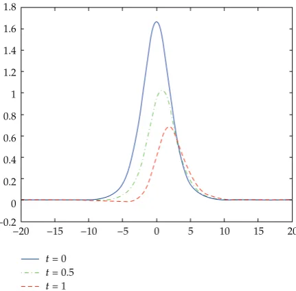
Figure 1:Whenτh0.05, the wave graph ofuat various times.

LetxL −20,xR 20,T 1.0, andυ γ 1. Since we do not know the exact solution of

1.4-1.5, an error estimates method in21 is used: a comparison between the numerical solutions on a coarse mesh and those on a refine mesh is made. We consider the solution on meshτ h1/160 as the reference solution. InTable 1, we give the ratios in the sense ofl∞ at various time steps.

Whenτ h0.05, a wave figure comparison ofuandρat various time steps is as in Figures1and2.

−0.2 0 0.2 0.4 0.6 0.8 1 1.2 1.4 1.6 1.8

t=0 t=0.5 t=1

−20 −15 −10 −5 0 5 10 15 20

Figure 2:Whenτh0.05, the wave graph ofρat various times.

Acknowledgments

The work of Jinsong Hu was supported by the research fund of key disciplinary of application

mathematics of Xihua University Grant no. XZD0910-09-1. The work of Youcai Xu was

supported by the Youth Research Foundation of Sichuan Universityno. 2009SCU11113.

References

1 C. E. Seyler and D. L. Fenstermacher, “A symmetric regularized-long-wave equation,”Physics of Fluids, vol. 27, no. 1, pp. 4–7, 1984.

2 J. Albert, “On the decay of solutions of the generalized Benjamin-Bona-Mahony equations,”Journal of Mathematical Analysis and Applications, vol. 141, no. 2, pp. 527–537, 1989.

3 C. J. Amick, J. L. Bona, and M. E. Schonbek, “Decay of solutions of some nonlinear wave equations,” Journal of Differential Equations, vol. 81, no. 1, pp. 1–49, 1989.

4 T. Ogino and S. Takeda, “Computer simulation and analysis for the spherical and cylindrical ion-acoustic solitons,”Journal of the Physical Society of Japan, vol. 41, no. 1, pp. 257–264, 1976.

5 V. G. Makhankov, “Dynamics of classical solitonsin non-integrable systems,”Physics Reports. Section C, vol. 35, no. 1, pp. 1–128, 1978.

6 P. A. Clarkson, “New similarity reductions and Painlev´e analysis for the symmetric regularised long wave and modified Benjamin-Bona-Mahoney equations,”Journal of Physics A, vol. 22, no. 18, pp. 3821– 3848, 1989.

7 I. L. Bogolubsky, “Some examples of inelastic soliton interaction,”Computer Physics Communications, vol. 13, no. 3, pp. 149–155, 1977.

8 B. Guo, “The spectral method for symmetric regularized wave equations,”Journal of Computational Mathematics, vol. 5, no. 4, pp. 297–306, 1987.

9 J. D. Zheng, R. F. Zhang, and B. Y. Guo, “The Fourier pseudo-spectral method for the SRLW equation,” Applied Mathematics and Mechanics, vol. 10, no. 9, pp. 801–810, 1989.

11 Y. D. Shang and B. Guo, “Legendre and Chebyshev pseudospectral methods for the generalized symmetric regularized long wave equations,”Acta Mathematicae Applicatae Sinica, vol. 26, no. 4, pp. 590–604, 2003.

12 Y. Bai and L. M. Zhang, “A conservative finite difference scheme for symmetric regularized long wave equations,”Acta Mathematicae Applicatae Sinica, vol. 30, no. 2, pp. 248–255, 2007.

13 T. Wang, L. Zhang, and F. Chen, “Conservative schemes for the symmetric regularized long wave equations,”Applied Mathematics and Computation, vol. 190, no. 2, pp. 1063–1080, 2007.

14 T. C. Wang and L. M. Zhang, “Pseudo-compact conservative finite difference approximate solution for the symmetric regularized long wave equation,”Acta Mathematica Scientia. Series A, vol. 26, no. 7, pp. 1039–1046, 2006.

15 T. C. Wang, L. M. Zhang, and F. Q. Chen, “Pseudo-compact conservative finite difference approximate solutions for symmetric regularized-long-wave equations,”Chinese Journal of Engineering Mathematics, vol. 25, no. 1, pp. 169–172, 2008.

16 Y. Shang, B. Guo, and S. Fang, “Long time behavior of the dissipative generalized symmetric regularized long wave equations,”Journal of Partial Differential Equations, vol. 15, no. 1, pp. 35–45, 2002.

17 Y. D. Shang and B. Guo, “Global attractors for a periodic initial value problem for dissipative generalized symmetric regularized long wave equations,” Acta Mathematica Scientia. Series A, vol. 23, no. 6, pp. 745–757, 2003.

18 B. Guo and Y. Shang, “Approximate inertial manifolds to the generalized symmetric regularized long wave equations with damping term,”Acta Mathematicae Applicatae Sinica, vol. 19, no. 2, pp. 191–204, 2003.

19 Y. Shang and B. Guo, “Exponential attractor for the generalized symmetric regularized long wave equation with damping term,”Applied Mathematics and Mechanics, vol. 26, no. 3, pp. 259–266, 2005.

20 F. Shaomei, G. Boling, and Q. Hua, “The existence of global attractors for a system of multi-dimensional symmetric regularized wave equations,” Communications in Nonlinear Science and Numerical Simulation, vol. 14, no. 1, pp. 61–68, 2009.