R E S E A R C H
Open Access
Optimal control for evolutionary imperfect
transmission problems
Luisa Faella
1and Carmen Perugia
2**Correspondence:
[email protected] 2Dipartimento di Scienze e
Tecnologie, Universitá del Sannio, Via Dei Mulini 59/A Palazzo Inarcassa, Benevento, 82100, Italia Full list of author information is available at the end of the article
Abstract
We study the optimal control problem of a second order linear evolution equation defined in two-component composites with
ε
-periodic disconnected inclusions of sizeε
in presence of a jump of the solution on the interface that varies according to a parameterγ
. In particular here the caseγ
< 1 is analyzed. The optimal control theory, introduced by Lions (Optimal Control of System Governed by Partial Differential Equations, 1971), leads us to characterize the control as the solution of a set of equations, called optimality conditions. The main result of this paper proves that the optimal control of theε
-problem, which is the unique minimum point of a quadratic cost functionalJε, converges to the optimal control of the homogenized problemwith respect to a suitable limit cost functionalJ∞. The main difficulties are to find the appropriate limit functional for the control of the homogenized system and to identify the limit of the controls.
MSC: Primary 49J20; 35B37; 35B27
Keywords: homogenization; optimal control; evolution equations
1 Introduction
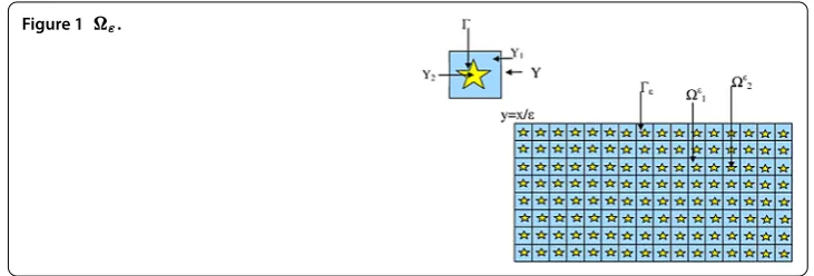
In this paper we study the optimal control of a linear hyperbolic problem with oscillating coefficients on a domainofRnmade up of two components, a connected one
εand
a second oneε, which is the union ofε-periodic disconnected inclusions of sizeε. On
the interfaceε=∂ε separating the two components, we prescribe the continuity of
the conormal derivatives and a jump of the solution proportional to the conormal deriva-tives through a function of orderεγ, meanwhile, a Dirichlet condition is imposed on the exterior boundary∂(see Figure ). The order of magnitude of this parameter, with re-spect to the periodε, determines the influence of the contact barrier in the propagation properties of the medium. Indeed this problem models the wave propagation in a medium made up of two components with very different coefficients of propagation, which gives rise to a jump in the boundary condition on the interface. This interface condition is the mathematical interpretation of imperfect interface characterized by the discontinuity of the displacement (see [–] and references therein).
This work connects the corresponding homogenization and correctors results proved respectively in [] and []. The first question of this paper deals with the existence of an optimal control of theε-problem with respect to a quadratic functional. If such a con-trol exists, the second and more interesting question is: does the optimal concon-trol of the ε-problem converge asε→ to the optimal control of the homogenized problem with
Figure 1 ε.
respect to a suitable cost functional? The optimal control of one or more aspects of a problem entails the minimization of a cost functional which describes physical quantities involved in the specific problem. To give a positive answer to both questions, we refer to the techniques used by Lions in []. These ones consist of the construction of the adjoint problem and the research of a set of equations, called optimality conditions, characterizing the optimal control and the related cost functional. As already shown by Hummel in [], for the homogenization results in the elliptic case, one cannot expect to have boundedness of the solutions whenγ > . Hence it would be natural here to supposeγ ≤. Neverthe-less in this paper we analyze the caseγ < being the caseγ = more delicate. Indeed it is already known from previous studies (see []) that the asymptotic behavior of the ε-problem differs in terms of the homogenized ε-problems in the two casesγ < andγ = . The second one is the most complicated one, since the limit problem is a coupled system of a P.D.E. and a O.D.E. and gives rise to what is called a memory effect. When searching an optimal control result for the caseγ = we cannot adapt the same arguments used for the more general caseγ < . In fact the homogenized problem is no more symmetric, hence the adjoint of the homogenized problem does not coincide with the limit of the adjoint problem atε-level. We will use other techniques to study the caseγ = .
The plan of the paper is as follows.
In Section we recall some useful properties of a specific functional space, introduced in [, ] by Donato and Monsurrò in the elliptic framework, suitable for the solutions of this kind of interface problems. Successively, we recall some further properties, involving evolution triples, needed in the time-dependent framework. They have been proved by Donatoet al.in [].
In Section , we state the main result, Theorem ., whose proof is performed into sev-eral steps. At first we describe the homogenization result for the hyperbolic problem; we refer the reader also to [] where all the proofs can be found. Then we study the control problem. Our approach to the optimal control problem for a hyperbolic equation consists in applying Pontryagin maximum principle to obtain the expression for the optimal con-trolwεat levelεin terms of the adjoint statepε, solution of the dual problem. We identify
the problem satisfied by the limit (u,w) of the sequence of optimal pairs{(uε,wε)}ε, where
uεdenotes the state of the system to be controlled, and also the problem satisfied by the
limitpof{pε}ε. We observe thatpis the adjoint state corresponding to an optimal control
properties for the sequence of the optimal controlswε. Finally, we prove that the limit of
the minimum points of the cost functionalJεat levelεis the minimum point of an
appro-priate limit cost functionalJ∞. Let us point out that the cost functionalJ∞ describe the physical properties of the wave equation for a composite occupying the whole, without any interface. Moreover, we observe that, without any technical difficulties, we can obtain the same optimal control result with a more general quadratic cost functional.
Optimal control problems and the exact controllability in domains with highly oscillat-ing boundary are considered in [–]. Moreover, we refer to [] for control of hyper-bolic problems with oscillating coefficients in a fixed domain and to [, ] for control of hyperbolic problems in perforated domains.
In [] and [] the authors study, respectively, the approximate control and the correctors for a class of parabolic equations with interfacial contact resistance. For the sake of com-pleteness, we recall also [] where all the results for transmission problems in the elliptic case are collected and [, ] where the authors treated the homogenization in other types of perforated domains. For the study of similar problems, where the same jump condition is taken into account, we quote here also [, , , –] and the references therein.
2 Statement of the problem and main result
Letbe an open bounded subset ofRn(n≥) andY= ],l
[× · · · ×],ln[ the reference cell.
We denote byYandYtwo nonempty open and disjoint subsets ofYsuch that
Y=Y∪Y,
withY connected and:=∂Y of classC. For anyk∈Znwe define the translated sets
Yk
i andkas follows:
Yik:=kl+Yi, k:=kl+,
wherekl= (kl, . . . ,knln) andi= , . Let{ε}be a sequence of positive real numbers con-verging to zero and for any givenεlet us set
Kε:=
k∈Zn|εk∩ =∅
.
Then we define the two components ofand the interface respectively as follows:
iε:=∩
k∈Kε εYik
, i= , , and ε:=∂ε.
We assume that
∂∩ k∈Zn
(εk)
:=∅. (.)
disjoint translated sets ofεY. Moreover,εis the interface separating the two components
with∂∪ε=∅(see Figure ).
In the sequel we denote by
•˜the zero extension to the whole ofof functions defined onεorε;
• χEthe characteristic function of any measurable setE∈Rn;
• mω(v) =ω ωv dxthe average on Y of any functionv∈L(ω).
Let us recall (see for instance []) that asε→, fori= , ,
χiε θi:= |Yi|
|Y| weakly inL
() (.)
θibeing the proportion of the material occupyingiε.
For anyε> , let us introduce he functional spaceVεas
Vε:=v∈H(ε)|v= on∂
,
which is a Banach space if endowed with the norm
vVε:=∇vL(
ε).
Clearly, since we do not assume any regularity on∂, the condition on∂in the defini-tion ofVεhas to be understood in a density sense. To be more precise,Vεis the closure,
with respect to theH(
ε)-norm, of the set of the functions inC∞(ε) with a compact
support contained in. This can be done in view of (.). For anyε> , we set
Wε:=v= (v,v)∈L
,T;Vε×L,T;H(ε)
|
v∈L,T;L(ε)
×L,T;L(ε)
, (.)
which is a Hilbert space if equipped with the norm
vWε=vL(,T;Vε)+vL(,T;H(
ε))+v
L(,T;L( ε))+v
L(,T;L( ε)).
LetAbe an×n Y-periodic matrix field with coefficients inL∞(Y) such that for anyλ∈Rn and a.e. inYone has
⎧ ⎪ ⎨ ⎪ ⎩
(A(x)λ,λ)≥α|λ|,
|A(x)λ| ≤β|λ|,
ai,j=aj,i for every ≤i,j≤n,
(.)
with <α<β.
Moreover, we suppose thathis aY-periodic function such that
h∈L∞() and∃h∈Rsuch that <h<h(y) a.e. in. (.)
For anyε> , we set
hε(x) :=h
x ε
and
Aε(x) :=A(x/ε). (.)
The aim of this paper is to study the optimal control and its asymptotic behavior asε→ for a hyperbolic imperfect transmission problem defined in the domainpreviously de-scribed.
More precisely letzε= (zε,zε) be a control to be found inL(,T;L(ε))×L(,T;
L(
ε)). For any fixedT> let us consider the following problem:
⎧ ⎪ ⎪ ⎪ ⎪ ⎪ ⎪ ⎪ ⎪ ⎪ ⎪ ⎪ ⎨ ⎪ ⎪ ⎪ ⎪ ⎪ ⎪ ⎪ ⎪ ⎪ ⎪ ⎪ ⎩
uε–div(Aε∇uε) =fε+zε inε×],T[,
uε–div(Aε∇u
ε) =fε+zε inε×],T[,
Aε∇u
ε·nε= –Aε∇uε·nε onε×],T[,
Aε∇u
ε·nε= –εγhε(uε–uε) onε×],T[,
uε= on∂×],T[,
uε() =Uε inε, uε() =Uε inε,
uε() =Uε inε, uε() =Uε inε,
(.)
whereγ < ,niεis the unitary outward normal toiε,i= , , and
⎧ ⎪ ⎨ ⎪ ⎩
(i) fε= (fε,fε)∈L(,T;L(ε))×L(,T;L(ε)),
(ii) Uε= (Uε,Uε)∈Vε×H(ε),
(iii) U
ε= (Uε,Uε)∈L(ε)×L(ε).
(.)
Let us introduce a class of function spaces expressly considered for the solution of this particular kind of interface problems. They were defined for the first time in [, ] and [] in the framework of the study of the analogous elliptic problem. Clearly, the space of the solutions must take into account either the geometry of the domain in which the material is confined or the boundary and interfacial conditions. For everyγ ∈R, we set (see also [])
Hε γ :=
v= (v,v)|v∈Vεandv∈H(ε)
.
The spaceHε
γ is a Banach space when equipped with the norm
v
Hγε:=∇v
L(
ε)+∇v
L( ε)+ε
γv
–vL(ε). It is easy to check that, if <ε< andγ≤γ, then
vHγε ≤ vHγε.
Moreover, for every fixedεthe norms ofHε
γ andVε×H(ε) are equivalent; see []
for details.
We point out that Hε
γ is a separable and reflexive Banach space dense in L(ε)×
L(
ε). Moreover,Hγε ⊆L(ε)×L(ε) with continuous imbedding. On the other
hand, one sees thatL(
space. This means that the triple (Hε
γ,L(ε)×L(ε), (Hγε)) is an evolution triple. We
refer the reader to [] for an in-depth analysis on this aspect. By using an approach to the evolutionary problems based on evolution triples, as far as the weak formulation of prob-lem (.) is concerned, we assume as precise formulation of formal probprob-lem the following one (see []):
⎧ ⎪ ⎪ ⎪ ⎪ ⎪ ⎪ ⎪ ⎪ ⎪ ⎪ ⎪ ⎨ ⎪ ⎪ ⎪ ⎪ ⎪ ⎪ ⎪ ⎪ ⎪ ⎪ ⎪ ⎩
finduε= (uε,uε) inWεsuch that
u
ε,v(Vε),Vε+u
ε,v(H(
ε)),H(ε)
+
εA
ε∇u
ε· ∇vdx+ εA
ε∇u
ε· ∇vdx
+εγ
εhε(uε–uε)(v–v)dσx= ε(fε+zε)vdx
+
ε(fε+zε)vdx ∀(v,v)∈V
ε×H(
ε) inD(,T),
uε() =Uε inε, uε() =Uε inε,
uε() =U
ε inε, uε() =Uε inε.
(.)
An abstract Galerkin method provides the existence and uniqueness result for the solution of problem (.) for anyε> and also somea prioriestimates (see []). We point out that the unique solutionuε(zε) of problem (.) is said the ‘state’ of the system to be controlled
and (.) are called ‘state equations’.
To any controlzε∈L(,T;L(ε))×L(,T;L(ε)) we associate the cost functional
Jε:L(,T;L(ε)×L(ε))→Rdefined in the following way:
Jε(zε) :=
T
ε
uε(zε)
+
T
ε
uε(zε)
+
T
ε |zε|+
T
ε
|zε|. (.)
This functional is continuous, strictly convex and coercive. Hence, by applying the direct method in the calculus of variations, the following minimum problem:
minJε(z) :z∈L
,T;L(ε)×L(ε)
(.)
admits a unique solutionwεwhich is called the optimal control of problem (.), (.) with
respect to the cost functional (.).
The aim of this paper is to study the asymptotic behavior, asε→ of the sequence of the optimal pairs (uε,wε) under the following assumptions on the data:
⎧ ⎪ ⎪ ⎪ ⎨ ⎪ ⎪ ⎪ ⎩
(i) U
ε U:= (U,U) weakly inL()×L(),
withU
∈H(),
(ii) U
ε U:= (U,U) weakly inL()×L(),
(iii) UεHγε ≤C,
(.)
withCpositive constant independent ofεand
fε f := (f,f) weakly inL
,T;L()×L,T;L(). (.)
LetA
(i) forγ < –
Aγλ=
|Y|
Y
A∇Wγdy (.)
withWγ ∈H(Y) a solution, for anyλ∈Rn, of
⎧ ⎪ ⎨ ⎪ ⎩
–div(A∇Wγ) = inY,
Wγ–λ·y Y-periodic,
|Y| Y(Wγ–λ·y)dy= ;
(.)
(ii) forγ = –
Aγλ=
|Y|
Y
A∇w+∇wdy (.)
with (w, w)∈H(Y
)×H(Y) a solution, for anyλ∈Rn, of
⎧ ⎪ ⎪ ⎪ ⎪ ⎪ ⎪ ⎪ ⎪ ⎨ ⎪ ⎪ ⎪ ⎪ ⎪ ⎪ ⎪ ⎪ ⎩
–div(A∇w) = inY ,
–div(A∇w) = inY,
(A∇w)·n
= –(A∇w)·n on,
–A∇w·n
=h(w– w),
w–λ·y Y-periodic,
|Y| Y(w
–λ·y)dy= ;
(.)
(iii) for – <γ <
Aγλ=
|Y|
Y
A∇wdy (.)
with w∈H(Y
) a solution, for anyλ∈Rn, of
⎧ ⎪ ⎪ ⎪ ⎨ ⎪ ⎪ ⎪ ⎩
–div(A∇w) = inY,
(A∇w)·n= on,
w –λ·y Y-periodic,
|Y| Y(w –λ·y)dy= .
(.)
We establish the following result.
Theorem . Letγ < and let Aεand hεsatisfy(.)-(.).Suppose that(.), (.),and
(.)hold and let wεthe optimal control of problem(.), (.), (.),and(.).Then
there exists a function w∈(L(,T;L()))such that
wε w= (w,w) in
L,T;L(), (.)
where
w=
θ
θ
andw
θ is the unique solution of the following problem:
min
T
u(z)+
T
|z|:z∈L,T;L(), (.)
u(z)being,for every z∈L(,T;L()),the unique solution of
⎧ ⎪ ⎪ ⎪ ⎨ ⎪ ⎪ ⎪ ⎩
u–div(A
γ∇u) =f+f+z in×],T[,
u= on∂×],T[,
u() =U+U in,
u() =U
+U in,
(.)
where the homogenized matrix A
γ is defined in(.), (.)and(.).
Remark . Forγ < – the matrix fieldA
γ is the classical one in a fixed domain. Forγ =
–, the homogenized matrixAγis described in terms of the periodic solution of an elliptic
problem posed in the two reference sub-domains of the periodicity cell and prescribing on the interface a conormal derivative proportional to the jump of the solution. Finally in the case – <γ< , the matrix fieldA
γ is the same obtained by Cioranescu and Saint Jean
Paulin in [], for the homogenization of the elliptic problem in the perforated domain εwith a Neumann condition on the boundary of the holes.
Remark . The boundness (iii) in (.) is necessary in order to havea prioriestimates for the solution of problem (.) and (.), as shown in Section below.
Remark . Iffiε=f|εi, withf ∈L
(), fori= , , then (.) holds withf
i=θif.
3 Proof of Theorem 2.1
This section is devoted to the proof of Theorem .. At first, we recall some convergence results about the sequence of solutions of problem (.) and (.). Then we give a char-acterization of the optimal controlwεatε-level in the form of the optimality system and
we deduce a uniform estimate forwε. Finally we identify the limit ofwεas the solution of
the optimality system related to the homogenized problem with respect to a suitable limit cost functional.
3.1 Asymptotic behavior of the
ε
-problemLetA
γ the matrix field defined in the previous section. We will make use of some
homog-enization results proved in [] that we recall below, for the reader’s convenience. For any fixedT> andγ < let us consider the following problem:
⎧ ⎪ ⎪ ⎪ ⎪ ⎪ ⎪ ⎪ ⎪ ⎪ ⎪ ⎪ ⎨ ⎪ ⎪ ⎪ ⎪ ⎪ ⎪ ⎪ ⎪ ⎪ ⎪ ⎪ ⎩
uε–div(Aε∇uε) =gε inε×],T[,
uε–div(Aε∇u
ε) =gε inε×],T[,
Aε∇u
ε·nε= –Aε∇uε·nε onε×],T[,
Aε∇u
ε·nε= –εγhε(uε–uε) onε×],T[,
uε= on∂×],T[,
uε() =Uε inε, uε() =Uε inε,
uε() =U
ε inε, uε() =Uε inε,
whereniεis the unitary outward normal toiε,i= , , and
⎧ ⎪ ⎨ ⎪ ⎩
(i) gε= (gε,gε)∈L(,T;L(ε))×L(,T;L(ε)),
(ii) U
ε= (Uε,Uε)∈V
ε×H( ε),
(iii) Uε= (Uε,Uε)∈L(ε)×L(ε).
(.)
Moreover, let us suppose that
⎧ ⎪ ⎪ ⎪ ⎨ ⎪ ⎪ ⎪ ⎩
(i) U
ε U:= (U,U) weakly inL()×L(),
withU∈H(), (ii) U
ε U:= (U,U) weakly inL()×L(),
(iii) U
εHγε ≤C,
(.)
withCpositive constant independent ofε, and
gε g:= (g,g) weakly inL
,T;L()×L,T;L(). (.)
Theorem .([]) Let Aε and hε satisfy(.)-(.).Suppose that(.), (.),and(.)
hold and let uεbe the solution of problem(.)and(.),withγ < .Then there exists an
extension operator Pε
∈L(L∞(,T;Hk(ε));L∞(,T;Hk())),for k= , ,such that
⎧ ⎪ ⎨ ⎪ ⎩
(i) Pε
uε u weakly* in L∞(,T;H()),
(ii) uε θu weakly* in L∞(,T;L()),
(iii) uε θu weakly* in L∞(,T;L()),
(.)
⎧ ⎪ ⎨ ⎪ ⎩
(i) Pε
uε u weakly* in L∞(,T;L()),
(ii) uε θu weakly* in L∞(,T;L()),
(ii) uε θu weakly* in L∞(,T;L()),
(.)
and
Aε∇uε+Aε∇uε Aγ∇u weakly* in L∞
,T;L()n, (.)
whereθandθare given by(.)and uis the unique solution in L(,T;H()),with u
in L(,T;L()),of the following problem:
⎧ ⎪ ⎪ ⎪ ⎨ ⎪ ⎪ ⎪ ⎩
u–div(Aγ∇u) =g+g in×],T[,
u= on∂×],T[,
u() =U+U in,
u() =U
+U in.
(.)
Moreover,if– <γ < ,
(i) Aε∇u
ε Aγ∇u weakly* in L∞(,T; [L()]n),
(ii) Aε∇u
ε weakly* in L∞(,T; [L()]n).
(.)
Remark .). We point out thatHε
γ ⊆L(ε)×L(ε) with continuous imbedding so
that the triple (Hε
γ,L(ε)×L(ε),Hγε) is an evolution triple (see Theorem . in []
for an in-depth analysis on this aspect).
Theorem . Let T∈], +∞[.Let Wεbe defined as in(.),hεand Aεas in(.)-(.).
For everyε,under assumptions(.), (.),and(.),problem(.)admits a unique weak solution uε∈Wε.Moreover,there exists a constant C,independent ofε,such that
uεL(,THε
γ(ε))+u
εL(,TL(
ε)×L(ε)) ≤CUεHε
γ +U
εL(
ε)×L(ε)+gεL(,T;L(ε)×L(ε))
. (.)
Let us point out that, for any fixedε, the solution of problem (.) and (.) has some further properties (see [], Chapter , Theorem .). In fact, under the same hypotheses of Theorem . the unique solutionuεof problem (.) and (.), withγ < satisfies
uε∈C
[,T];Hγε
, uε∈C
[,T];L(ε)×L(ε)
(.)
and
uεL∞(,THγε(ε))+u
εL∞(,TL(
ε)×L(ε)) ≤CUεHε
γ +U
εL(
ε)×L(ε)+gεL(,T;L(ε)×L(ε))
, (.)
whereCis the same constant as in (.).
3.2 The optimality system
The following results give a characterization of the optimal controls for both problem at levelεand homogenized problem (.) (see [], Chapter ).
Theorem . For every ε, under assumptions (.)-(.) and (.), the optimal pair (uε,wε),solution of problem(.), (.), (.),and(.)is characterized by the
follow-ing optimality system: ⎧
⎪ ⎪ ⎪ ⎪ ⎪ ⎪ ⎪ ⎪ ⎪ ⎪ ⎪ ⎨ ⎪ ⎪ ⎪ ⎪ ⎪ ⎪ ⎪ ⎪ ⎪ ⎪ ⎪ ⎩
uε–div(Aε∇u
ε) =fε+wε inε×],T[,
uε–div(Aε∇uε) =fε+wε inε×],T[,
Aε∇u
ε·nε= –Aε∇uε·nε onε×],T[,
Aε∇u
ε·nε= –εγhε(uε–uε) onε×],T[,
uε= on∂×],T[,
uε() =Uε inε, uε() =Uε inε,
uε() =Uε inε, uε() =Uε inε,
(.)
⎧ ⎪ ⎪ ⎪ ⎪ ⎪ ⎪ ⎪ ⎪ ⎪ ⎪ ⎪ ⎨ ⎪ ⎪ ⎪ ⎪ ⎪ ⎪ ⎪ ⎪ ⎪ ⎪ ⎪ ⎩
pε–div(Aε∇pε) =uε inε×],T[,
pε–div(Aε∇p
ε) =uε inε×],T[,
Aε∇p
ε·nε= –Aε∇pε·nε onε×],T[,
Aε∇p
ε·nε= –εγhε(pε–pε) onε×],T[,
pε= on∂×],T[,
pε(T) = inε, pε(T) = inε,
pε(T) = inε, pε(T) = inε,
pε= –wε a.e. in],T[×ε. (.)
As previously, we prefer to use the following weak formulation of problems (.) and (.): ⎧ ⎪ ⎪ ⎪ ⎪ ⎪ ⎪ ⎪ ⎪ ⎪ ⎪ ⎪ ⎨ ⎪ ⎪ ⎪ ⎪ ⎪ ⎪ ⎪ ⎪ ⎪ ⎪ ⎪ ⎩
finduε= (uε,uε) inWεsuch that
u
ε,v(Vε),Vε+u
ε,v(H(
ε)),H(ε)
+
εA
ε∇u
ε· ∇vdx+ εA
ε∇u
ε· ∇vdx
+εγ
εhε(uε–uε)(v–v)dσx= ε(fε+wε)vdx
+
ε(fε+wε)vdx for every (v,v)∈V
ε×H(
ε) inD(,T),
uε() =Uε inε, uε() =Uε inε,
uε() =Uε inε, uε() =Uε inε,
(.) and ⎧ ⎪ ⎪ ⎪ ⎪ ⎪ ⎪ ⎪ ⎪ ⎪ ⎪ ⎪ ⎨ ⎪ ⎪ ⎪ ⎪ ⎪ ⎪ ⎪ ⎪ ⎪ ⎪ ⎪ ⎩
findpε= (pε,pε) inWεsuch that
p
ε,v(Vε),Vε+p
ε,v(H(
ε)),H(ε)
+
εA
ε∇p
ε· ∇vdx+ εA
ε∇p
ε· ∇vdx
+εγ
εhε(pε–pε)(v–v)dσx= εuεvdx dt
+
εuεvdx dt for every (v,v)∈V
ε×H(
ε) inD(,T),
pε(T) = inε, pε(T) = inε,
pε(T) = inε, pε(T) = inε.
(.)
Let us consider the cost functionalJ∞:L(,T;L())→Rdefined in the following way:
J∞(z) :=
T
u(z) + T
|z|, (.)
where for every controlz∈L(,T;L()),u(z) is the unique solution of problem (.).
This functional is continuous, strictly convex, and coercive. Hence, by applying the direct method in the calculus of variations, the minimum problem (.) admits a unique solu-tionw¯ which is the optimal control of problem (.) with respect to the cost functional (.).
Theorem . The optimal pair(u,w),¯ solution of problem(.)and(.)is
character-ized by the following optimality system:
⎧ ⎪ ⎪ ⎪ ⎨ ⎪ ⎪ ⎪ ⎩
u–div(Aγ∇u) =f+f+w¯ in×],T[,
u= on∂×],T[,
u() =U+U in,
u() =U
+U in,
(.) ⎧ ⎪ ⎪ ⎪ ⎨ ⎪ ⎪ ⎪ ⎩
p–div(A
γ∇p) =u in×],T[,
u= on∂×],T[,
p(T) = in,
p(T) = in,
(.)
3.3 A prioriestimates
In this subsection, we deduce somea priorinorm-estimates either for the sequence of the optimal controlswεor for the corresponding solutionuε=uε(wε) (resp.pε=pε(uε)) of
problem (.) (resp. (.)).
Proposition . Let(uε,wε)∈(L(,T;L(ε)×L(ε)))be the optimal pair,solution
of the optimality system(.), (.)and(.).Under assumptions(.)-(.), (.)and (.),there exists a constant c,independent ofε,such that
wεL(,T;L(
ε)×L(ε))≤c, (.)
uεL(,T;L(
ε)×L(ε))≤c, (.)
for everyε.
Proof Let us fixε. Letuε=uε(wε) be the unique solution of problem (.) andpε=pε(uε)
be the unique solution of the adjoint problem (.). Choosingpεas test function in (.)
anduεas a test function in (.), we have
T
uε(t,·),pε(t,·)
(H(
ε)),H(ε)dt+ T
uε(t,·),pε(t,·)
(H(
ε)),H(ε)dt +
T
ε
A∇xuε∇xpε+uεpεdx dt+
T
ε
A∇xuε∇xpε+uεpεdx dt
= T
ε
fεpε+wεpεdx dt+
T
ε
fεpε+wεpεdx dt (.)
and
T
pε(t,·),uε(t,·)
(H(
ε)),H(ε)dt+ T
pε(t,·),uε(t,·)
(H(
ε)),H(ε)dt +
T
ε
A∇xpε∇xuε+pεuεdx dt+
T
ε
A∇xpε∇xuε+pεuεdx dt
= T
ε
(uε)dx dt+
T
ε
(uε)dx dt. (.)
Integrating by parts, we get
T
uε(t,·),pε(t,·)
(H(
ε)),H(ε)dt+ T
uε(t,·),pε(t,·)
(H(
ε)),H(ε)dt =uε(T),pε(T)
(H(
ε)),H(ε)–
uε(),pε()
(H(
ε)),H(ε) –
T
uε(t,·),pε(t,·)
L(
ε)dt+
uε(T),pε(T)
(H(
ε)),H(ε) –uε(),pε()
(H(
ε)),H(ε)– T
uε(t,·),pε(t,·)
L(
and T
pε(t,·),uε(t,·)
(H(
ε)),H(ε)dt+ T
pε(t,·),uε(t,·)
(H(
ε)),H(ε)dt =pε(T),uε(T)
(H(
ε)),H(ε)–
pε(),uε()
(H(
ε)),H(ε) –
T
pε(t,·),uε(t,·)
L(
ε)dt+
pε(T),uε(T)
(H(
ε)),H(ε) –pε(),uε()
(H(
ε)),H(ε)– T
pε(t,·),uε(t,·)L(
ε)dt. (.)
Subtracting (.) from (.), using (.) and (.), the symmetry of the matrixA, the initial conditions in (.), and the final conditions in (.), we obtain
pε(),Uε
(H(
ε)),H(ε)–
Uε,pε()
(H(
ε)),H(ε) +pε(),Uε
(H(
ε)),H(ε)–
Uε,pε()
(H(
ε)),H(ε) =
T
ε
fεpε+wεpε–uεdx dt+
T
ε
fεpε+wεpε–uεdx dt.
By virtue of (.), as a result we find T
ε
uε+wεdx dt+
T
ε
uε+wεdx dt
= – T
ε
fεwεdx dt–
T
ε
fεwεdx dt
+
ε
Uεpε() –Uεpε()dx+
ε
Uεpε() –Uεpε()dx, (.)
from which, by the Cauchy-Schwarz inequality, it follows that
uεL(,T;L(
ε)×L(ε))+wε
L(,T;L(
ε)×L(ε)) ≤ wεL(,T;L(
ε)×L(ε))fεL(,T;L(ε)×L(ε)) +UεL(
ε)×L(ε)p
ε(,·)L(
ε)×L(ε) +UεL(
ε)×L(ε)pε(,·)L(ε)×L(ε). (.) On the other hand, to estimatepε(,·)L(
ε)×L(ε)andp
ε(,·)L(
ε)×L(ε)let us apply Theorem . withpεinstead ofuε. Then by translation we get
pε(,·)H(
ε)+p
ε(,·)L(
ε)≤CuεL(,T;L(ε)×L(ε)), (.) whereCis a constant independent ofε. Finally, combining (.) with (.) and using (.), as a result we find that
uεL(,T;L(
ε)×L(ε))+wε
L(,T;L(
ε)×L(ε)) ≤cwεL(,T;L(
As a consequence of (.), up to a subsequence still denoted byε, we have the following convergences:
wε w inL
,T;L(),
wε w inL
,T;L().
(.)
3.4 Conclusions
Let us recall that for the adjoint state atε-levelpε= (pε,pε), the following convergences
hold:
pε θp weakly* inL∞
,T;L(),
pε θp weakly* inL∞
,T;L().
Hence by (.) and (.) we get
θp= –w,
θp= –w,
whereθandθare given in (.). As a consequence
w=
θ
θ
w, (.)
which is (.).
Hence we are able to pass to the limit, asεgoes to , in the optimality system (.)-(.) by applying Theorem . to both problems (.) and (.) with, respectively,gε=fε+wε
andgε=uε. Then by (.), (.), and (.) asθ+θ= , we see that the pair (u,wθ) is
such that ⎧ ⎪ ⎪ ⎪ ⎨ ⎪ ⎪ ⎪ ⎩
u–div(A
γ∇u) =f+f+θw in×],T[,
u= on∂×],T[,
u() =U+U in,
u() =U
+U in,
(.)
⎧ ⎪ ⎪ ⎪ ⎨ ⎪ ⎪ ⎪ ⎩
p–div(A
γ∇p) =θu+θu=u in×],T[,
u= on∂×],T[,
p(T) = in,
p(T) = in,
(.)
p= –
θ
w. (.)
Finally, by Theorem . and uniqueness we get w
θ =w¯ and the convergences (.)-(.)
and (.) hold for the whole sequence. Hence Theorem . is now completely proved.
Competing interests
Authors’ contributions
The authors conceived and wrote this article in collaboration and with the same responsibility. All of them read and approved the final manuscript.
Author details
1Dipartimento di Ingegneria Elettrica e dell’ Informazione, Università degli Studi di Cassino e del Lazio Meridionale, via
G. Di Biasio 43, Cassino, FR 03043, Italia.2Dipartimento di Scienze e Tecnologie, Universitá del Sannio, Via Dei Mulini 59/A Palazzo Inarcassa, Benevento, 82100, Italia.
Received: 17 November 2014 Accepted: 4 March 2015 References
1. Auriault, JL, Ene, H: Macroscopic modelling of heat transfer in composites with interfacial thermal barrier. Int. J. Heat Mass Transf.37, 2885-2892 (1994)
2. Canon, E, Pernin, JN: Homogenization of diffusion in composite media with interfacial barrier. Rev. Roum. Math. Pures Appl.44, 23-36 (1999)
3. Donato, P: Some corrector results for composites with imperfect interface. Rend. Mat. Appl. (7)26, 189-209 (2006) 4. Donato, P: Homogenization of a class of imperfect transmission problems. In: Damlamian, A, Miara, B, Li, T (eds.)
Multiscale Problems: Theory, Numerical Approximation and Applications. Series in Contemporary Applied Mathematics CAM, vol. 16, pp. 109-147. Higher Education Press, Beijing (2011)
5. Donato, P, Faella, L, Monsurrò, S: Homogenization of the wave equation in composites with imperfect interface: a memory effect. J. Math. Pures Appl.87, 119-143 (2007)
6. Donato, P, Faella, L, Monsurrò, S: Correctors for the homogenization of a class of hyperbolic equations with imperfect interfaces. SIAM J. Math. Anal.40, 1952-1978 (2009)
7. Donato, P, Jose, E: Corrector results for a parabolic problem with a memory effect. ESAIM: Math. Model. Numer. Anal.
44, 421-454 (2010)
8. Donato, P, Jose, E: Asymptotic behavior of the approximate controls for parabolic equations with interfacial contact resistance. ESAIM Control Optim. Calc. Var.21, 138-164 (2015). doi:10.1051/cocv/2014029
9. Donato, P, Monsurrò, S: Homogenization of two heat conductors with interfacial contact resistance. Anal. Appl.2, 247-273 (2004)
10. Monsurrò, S: Erratum for the paper ‘Homogenization of a two-component composite with interfacial thermal barrier’. Adv. Math. Sci. Appl.14, 375-377 (2004)
11. Lions, JL: Optimal Control of System Governed by Partial Differential Equations. Springer, Berlin (1971)
12. Hummel, HC: Homogenization for heat transfer in polycrystals with interfacial resistances. Appl. Anal.75, 403-424 (2000)
13. Monsurrò, S: Homogenization of a two-component composite with interfacial thermal barrier. Adv. Math. Sci. Appl.
13, 43-63 (2003)
14. De Maio, U, Gaudiello, A, Lefter, C: Optimal control for a parabolic problem in a domain with highly oscillating boundary. Appl. Anal.83(12), 1245-1264 (2004)
15. De Maio, U, Faella, L, Perugia, C: Optimal control problem for an anisotropic parabolic problem in a domain with very rough boundary. Ric. Mat.63(2), 307-328 (2014)
16. De Maio, U, Faella, L, Perugia, C: Optimal control for a second-order linear evolution problem in a domain with oscillating boundary. Complex Var. Elliptic Equ. doi:10.1080/17476933.2015.1022169 (to appear)
17. De Maio, U, Nandakumaran, AK, Perugia, C: Exact internal controllability for the wave equation in a domain with oscillating boundary with Neumann boundary condition. Evol. Equ. Control Theory (2015, to appear)
18. Durante, T, Faella, L, Perugia, C: Homogenization and behaviour of optimal controls for the wave equation in domains with oscillating boundary. NoDEA Nonlinear Differ. Equ. Appl.14(5-6), 455-489 (2007)
19. Durante, T, Mel’nyk, TA: Asymptotic analysis of an optimal control problem involving a thick two-level junction with alternate type of controls. J. Optim. Theory Appl.144(2), 205-225 (2010)
20. Durante, T, Mel’nyk, TA: Homogenization of quasilinear optimal control problems involving a thick multilevel junction of type 3:2:1. ESAIM Control Optim. Calc. Var.18(2), 583-610 (2012)
21. Lions, JL: Contrôlabilité Exacte et Homogénéisation. I. Asymptot. Anal.1(1), 3-11 (1988)
22. Cioranescu, D, Donato, P: Exact internal controllability in perforated domains. J. Math. Pures Appl.68(2), 185-213 (1989)
23. Cioranescu, D, Donato, P, Zuazua, E: Exact boundary controllability for the wave equation in domains with small holes. J. Math. Pures Appl.71(4), 343-377 (1992)
24. Donato, P, Nabil, A: Homogenization and correctors for the heat equation in perforated domains. Ric. Mat.50(1), 115-144 (2001)
25. Faella, L, Perugia, C: Homogenization of a Ginzburg-Landau problem in a perforated domain with mixed boundary conditions. Bound. Value Probl.2014, 223 (2014). doi:10.1186/s13661-014-0223-2
26. Lipton, R: Heat conduction in fine scale mixtures with interfacial contact resistance. SIAM J. Appl. Math.58, 55-72 (1998)
27. Lipton, R, Vernescu, B: Composite with imperfect interface. Proc. R. Soc. Lond. Ser. A452, 329-358 (1996) 28. Monsurrò, S: Homogenization of a composite with very small inclusions and imperfect interface. In: Multi Scale
Problems and Asymptotic Analysis. GAKUTO Internat. Ser. Math. Sci. Appl., vol. 24, pp. 217-232. Gakk ¯otosho, Tokyo (2006)
29. Yang, Z: Homogenization and correctors for the hyperbolic problems with imperfect interfaces via the periodic unfolding method. Commun. Pure Appl. Anal.13(1), 249-272 (2014)
30. Yang, Z: The periodic unfolding method for a class of parabolic problems with imperfect interfaces. ESAIM: Math. Model. Numer. Anal.48(5), 1279-1302 (2014)
32. Faella, L, Monsurrò, S: Memory effects arising in the homogenization of composites with inclusions. In: Topics on Mathematics for Smart System, pp. 107-121. World Scientific, Hackensack (2007)
33. Cioranescu, D, Saint Jean Paulin, J: Homogenization in open sets with holes. J. Math. Anal. Appl.71, 590-607 (1979) 34. Zeidler, E: Nonlinear Functional Analysis and Its Applications. Vol II, Part A and B. Springer, Berlin (1980)