ANALYSIS OF CHANGES IN SOIL VOLUMETRIC WATER CONTENT USING COMMON-OFFSET GPR Dr. Hussein H. Karim*, Dr. Hasan H. Joni, Aram A. Dawood

[Karim et al., 3(9): September, 2016] ISSN 2349-4506

Impact Factor: 2.785

G

lobal

J

ournal of

E

ngineering

S

cience and

R

esearch

M

anagement

ANALYSIS OF CHANGES IN SOIL VOLUMETRIC WATER CONTENT USING

COMMON-OFFSET GPR

Dr. Hussein H. Karim*, Dr. Hasan H. Joni, Aram A. Dawood

*

Professor, Building and Construction Engineering Department, University of Technology, Baghdad,

Iraq

Asst. Professor, Building and Construction Engineering Department, University of Technology,

Baghdad, Iraq

M.Sc. in Transportation Engineering, Department of Building and Construction Engineering,

University of Technology, Baghdad, Iraq

DOI:

KEYWORDS

: GPR, Common-offset, Pavement subbase-subgrade, volumetric water content.

ABSTRACT

In highway engineering, GPR is a nondestructive tool for prediction pavement layers conditions, the quality of subgrade soils, and assessing other pavement conditions, such as moisture-related pavement damage. From the reflected GPR wave information, dielectric properties of the materials, which are highly dependent on soil or aggregate-water-air systems, can be estimated. An increase in dielectric constant may indicate an increase in moisture content of dielectric materials. However, the relationship between dielectric value and moisture content is complex and controlled by many factors. GPR studies, which consider both real and imaginary parts of dielectric value and its frequency dependent behavior, have shown potentials for developing more robust model to predict moisture content. This paper presents an overview of ground coupled GPR capabilities in estimating water content that is necessary in assessing pavement condition. Two types of antennas (800 and 500 MHz) were employed to decide the best monitoring for the water seepage under new or existing pavements. As well as, the data outcomes will be presented with the necessary data filtration and post processing softwares to observe spectrums behavior during the wetting cycles. Finally, it is concluded that estimation of soil water content using Common-Offset GPR measurements mode facilitates rapid data acquisition.

INTRODUCTION

In highway researches, the accurate measurement of the soil water content and its changes is of vital issue, as they affect significantly the soil strength and its deformation characteristics, and in turn influencing the stabilization of the surface constructions, subsidence and ground water flow. In pavement engineering, for effective design of subsurface pavement layers, non-destructive methods are crucial to observe changes in soils water contents. Ground Penetrating Radar (GPR) is one of the non-destructive geophysical methods for subsurface measurement. It is an effective tool to gain a lot of information after its data interpretation such as soil water content. This can be done after determining dielectric constant from the transmission velocity of the impulse electromagnetic wave, and using empirical relationships to estimate the soil water content and its changes (Saito and Kitahara, 2012; Zhang, 2012).

[Karim et al., 3(9): September, 2016] ISSN 2349-4506

Impact Factor: 2.785

G

lobal

J

ournal of

E

ngineering

S

cience and

R

esearch

M

anagement

The main objective of this paper is to introduce the capacity of surface GPR to rapidly and non-invasively estimate the volumetric water content that is important for assessing pavement condition. This new approach analyzes the amplitude attributes of the GPR pulse obtained from conventional single-offset surface-coupled profiling.

PARAMETERS AFFECTED BY MOISTURE ACCUMULATION

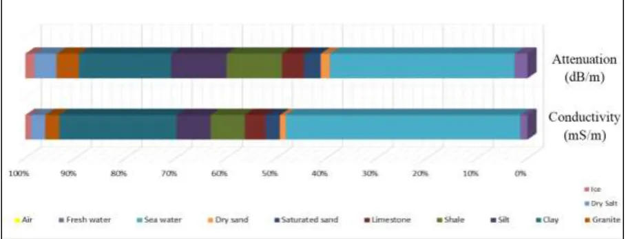
The most important material electrical properties are the dielectric constant and the conductivity. Both are greatly influenced by water (e.g. material moisture content). For example, the soil conductivity limits the maximum depth of energy penetration since it influences the rate of which the energy is absorbed. A more conductive soil (one that is wetter or has a higher clay content) will absorb the energy at a far greater rate than a low conductivity soil such as dry sand (Griffin et al., 2002).

The electric conductivity describes the ability of a material to pass free electric charges under the influence of an applied field. The primary effect of conductivity on EM waves is energy loss, which is expressed as the real part of the conductivity. The imaginary part contributes to energy storage and the effect is usually much less than that of energy loss (Cassidy, 2009). The least penetration occurs in saturated clayey materials or where the moisture content is saline. In addition, to understand the behavior of different materials, sketched scalar bars combine both attenuation (dB/m) and conductivity (mS/m) in different materials are presented in Figure 1.

Figure 1: Scalar bars showing the variation of conductivity and attenuation for materials.

The dielectric permittivity of a substance refers to its ability to store (i.e. permit) an electric field that has been applied to it. The permittivity of a material is a complex function having both real and imaginary parts, with the real and imaginary components affects the wave speed and wave absorption, respectively. Moreover, because the conduction loss is usually much higher than dielectric effect loss, the dielectric constant can be considered a real number (Evans, et al. 2007). This is convenient for the approximate calculation of radar wave velocities and wavelengths.

The dielectric constant is commonly normalized with respect to the permittivity of free space, and is referred to as the relative dielectric constant( Saarenketo, 1997).

εr* = εr'- iεr''' (1)

This can be further divided into the high frequency loss components

εr* = εr' -i [εr'' +

σ

𝜔𝜀𝑜 ] (2) where εr* is the relative complex dielectric permittivity of the medium, εr' is the real part of the dielectric

[Karim et al., 3(9): September, 2016] ISSN 2349-4506

Impact Factor: 2.785

G

lobal

J

ournal of

E

ngineering

S

cience and

R

esearch

M

anagement

conductivity of the medium (mho/m) or (S/m), ω f (rad/sec), and εo is the dielectric

permittivity of free space = 8.854 x 10-12 _Farad/m.

The bar chart shown in Figure 2 summarizes the selection of classified and reorganized values for a variety of materials relating to several researches (Hubbard, 1997; Hothan et al., 2000; Saarenketo, 2000; Maierhofer, 2003; Saarenketo, 2006; and Evans, 2007).

MOISTURE SURVEY FROM GPR BASIS

The data are analyzed by tracking the amplitude of the reflection from above the layered portion of the irrigation pipes, since the radiation travels through the medium and reproduced back to the receiver, this can be exploited by making a massive scope to estimate the dielectric constant by the hyperbola fitting. From the arrival time of the EM wave, it is possible to estimate the EM wave velocity in the soil if the wave travel path is known by reflecting from an object. At the frequency range usually used in GPR, the EM wave velocity depends strongly on the electric properties of the material that is the relative permittivity, as shown in equation (3) and simplified to equation (4).

𝑉𝑚= 𝑐/√{( 𝜀𝑟𝜇𝑟

2 )} [(1 + 𝑃

2_{) + 1] (3)}

where P is the loss factor and equals to σ/ωεr, c is the velocity of light in vacuum c = 299,792,458 m/sec. In

addition, the radar signal velocity in low-loss materials (P≈ 0) which are amenable to radar sounding is related to εr (Davis and Annan, 1989).

𝑉𝑚= 𝑐

√ε𝑟 (4)

The relative permittivity of water is about 81, while that of soil particles is about 3 to 10 and that of air is 1. This indicates that the relative permittivity of the soil is very sensitive to its moisture content (Huisman et al., 2003). GPR surveys on pavement moisture content can be divided into two parts: the first considers water content in subgrade soils and unbound base, the other concerns the water contentwithin pavement construction materials. Since time-domain reflectometry (TDR) has already been accepted as a reliable method for soil water content the method that were used in TDR to relate water content and dielectric constant focuses on establishing empirical relationships between volumetric water content and dielectric constant of soil. The most commonly used model was developed by Topp et al. (1980), which is a third-order polynomial relationship, given by equation (5):

θv = -5.3 x 10-2 +2.92 x 10-2 Ka -5.5 x 10-4 Ka2 + 4.3 x 10-6 Ka3 (5)

[Karim et al., 3(9): September, 2016] ISSN 2349-4506

Impact Factor: 2.785

G

lobal

J

ournal of

E

ngineering

S

cience and

R

esearch

M

anagement

Figure 2: Characteristic values of the dielectric constant for a variety of materials.

MODEL PREPARATION AND DATA COLLECTION

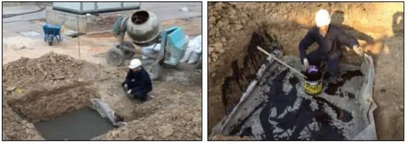
The study was first planned to be conducted at the University of Technology (Figs. 3 and 4). But, the difficulties represented by the elevated ground water table (around 90 cm in depth) made the continuation of this work impossible. Following the same procedures achieved in the previous site, the case study was revised near to the Army Canal with dimensions admitted (2.5 × 2.25 × 0.6 m) hole. The model consists four molded concrete walls using lubricated wood and steel templates and the bottom base casted with 1: 2: 4 percentages. All corners were sealed with mastic asphalt brought from Al-Daura Refinery to prevent any moisture ingress (Fig. 5a and b).

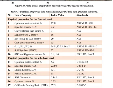
The next stage comprises the placement of 30 cm of air-dried soil and 20 cm air-dried sub-base (type B) (their properties are shown in Table 1). The arrangement of the irrigation pipes within the proposed model with its necessary dimensions are shown in the schematic Figure 6.

(a) (b)

[Karim et al., 3(9): September, 2016] ISSN 2349-4506

Impact Factor: 2.785

G

lobal

J

ournal of

E

ngineering

S

cience and

R

esearch

M

anagement

(a) (b) (c)

Figure 4: Field model preparation for subgrade placement, compaction and model demolition.

(a) (b) (c) Figure 5: Field model preparation procedures for the second site location.

Table 1: Physical properties and classification for the fine and granular soil used.

No. Index Property Index Value Standards Physical properties for the fine soil used

1 Optimum water content % 17.8 ASTM: D - 698

2 Specific gravity (G.S) 2.71 ASTM: D -854 -14

4 Gravel (larger than 2mm) % 0 N/A

5 Sand (0.06 to 2 mm) % 16 N/A

6 Silt (0.005 to 0.06 mm) % 29 N/A

7 Clay (less than 0.005 mm) % 55 N/A

8 (L.L, P.L, P.I) % 34.8 ,17.35, 16.42 ASTM: D -4318-10

9 Soil Symbols (USCS) CL ASTM: D2487-11

10 SO3 and Gypsum contents % 0.9, 1.6 BSI 1377, Part 3

Physical properties for the sub- base used

11 Optimum water content % 5.2 D 1557-12

12 Specific gravity (G.S) 2.350 D 854-14

13 Liquid Limit (L.L. %) 33.1 D 2487

14 Plastic Limit (P.L. %) 18 D 3282

15 SO3 Content % 0.142 BSI 1377, Part 3

16 Gypsum content % 0.35 BSI 1377, Part 3

[Karim et al., 3(9): September, 2016] ISSN 2349-4506

Impact Factor: 2.785

G

lobal

J

ournal of

E

ngineering

S

cience and

R

esearch

M

anagement

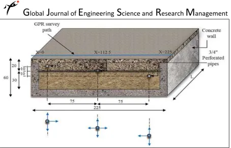
Figure 6: Schematic diagram cross-section of the pumping model and layers with the irrigation directions (all dimensions are in cm).

For alignments and specifications for the pipes system used, three (3/4 inch) diameter perforated CPVC pipes Sc.80 wp.690 psi conform to ASTM F 441/F 441M were used, with water pressure rating according to the diameter, 690 psi (4760 kPa). One irrigation side of each CPVC pipe was connected to (female fitting Adapters 90° Elbows) that connects to the high pressure hose pipes using male hose fitting and directing to high pressure Brass impeller water pump. The second side of the pipes were closed using high quality fitting congeal. To avoid any clogging at the perforation inlets, a thin tissue mesh with very fine opening close to 0.075 mm used for enveloping the pipes before installing in the appropriate location.

In order to monitor movements of wetting fronts in the model, time-lapse common offset (i.e. the transmitter and receiver are kept at fixed antenna offset of 18 and 14 cm for 800 and 500 MHz antennas respectively). This acquisition mode facilitates rapid data acquisition at walking speed. For all measurements, the traces were acquired in different intervals at initial state of pumping 15, 30, 60 minutes after immediate pumping. After this period, profiles were then collected at 180, 360, and 720 minutes after pumping was ceased. One survey was finally collected at 1440 minutes (24 hr.) by pumping 1500 ml of water. The pumping cycle was repeated after three-four days until the 4th cycle is included. Figure 7 shows a two dimensional radargram for the initial state (before water irrigation) with 500 and 800 MHz, respectively.

(a) (b)

[Karim et al., 3(9): September, 2016] ISSN 2349-4506

Impact Factor: 2.785

G

lobal

J

ournal of

E

ngineering

S

cience and

R

esearch

M

anagement

RESULTS, INTERPRETATION AND DISCUSSION

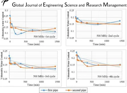
Figure 8 displays the common offset (CO) profiles acquired at initial, 15, 30, 60, 180, 360, 720 and 1440 minutes for the second irrigation cycle. As it is depicted from overall radargrams, the horizontal separation is noticeable between the two pipes about 0.75 m with time window 2.5 and 4 ns respectively. The third pipe is seemed to be difficult to observe at initial irrigation cycles, this may have two explanations; the first may confirm with the concept of the waves attenuation caused by the soil type specifically for clayey soils, while the second as the CPVC pipe material has a lower electrical conductivity that prevents emitting high radiation as irons or other reflective metals. The third pipe gives slight reflections after performing the following filters: DC removal, amplitude correction, and the band-pass filtering by increasing the low pass and the high pass in MHz.

The second attempt of irrigation cycles represents the irrigation intervals from the initial state immediately after water pumping, which are accumulatively measured. For all stages, the radargrams include the first two pipes, the first placed within the subbase at 10 cm depth and the second between the subgrade–subbase interface boundary, which is clearly appeared due to materialistic property difference at approximate 5 ns or 20 cm from the surface.

As depicted for all profiles attempts (Figure 8), the first horizontal strong signal accounts for the pulse wave traveled directly between two antennas. This kind of wave is referred to as a direct wave. Because of the velocity of air wave is equal to the speed of light in the vacuum, an actual travel time can be calculated if the antenna separation is fixed. Then the air wave arrival time can be used to calibrate time zero of the profile data.

At initial Common-offset profile (Figure 8a), there is distinct strong signal beneath the first pipe hyperbolic shape. Another strong signal inclined at the top of the second pipe extending through the interface boundary towards the first pipe approximately from 0.75 to 1.1 m, this may point for the water emitted from the right-side direction of the first pipe combined with the actual emitting water of the second pipe itself.

During the first hour and after the initial pumping, both the two mentioned strong signals are being progressively bleached out, this is strong indication that the distribution or the movement of the injected water is greater within the initial periods, Figures (8a to d).

After 24 hours, the pipes hyperbolas become more evident, in addition the profile present more homogeneous masses, which may be due to the moisture content of the soil is near to be uniform inside the bounded model. That means the velocity of the EM wave also becomes approximately constant within specific masses. In such a situation, the reflected signals from the horizontal boundary between the subbase and the subgrade become more clearly horizontal, note the boundary in Figure 8h.

The hyperbolic shape signals peaked at the location of pipes when the antenna is directly above it, in this experiment, the irrigation pipe is a point reflection source and this reflection will be greater or more duplicated when the conductivity of the medium increases or at high reflective bodies. Hence, when the water concentration is high at specific locations, the hyperbola reflection seemed to be located with less travel time (closer to surface) for both irrigation pipes, Figures (8a to f).

Table 2 presents the data outcomes for the second irrigation cycle using 800 and 500 MHz frequencies. The first column represents the time of irrigation intervals and the rest columns represent the average dielectric constants from which the volumetric water contents of the medium are obtained for the first two pipes.

During the survey using 800 MHz frequency, the water content values or the dielectric permittivity for the upper pipe were found to have lower water content values in compare to the second pipe, slight deviations were noticed in the first irrigation cycle throughout the first intervals. These deviations become more noticeable after 12 and 24 hours. For example, the water content values were found to be about 17.8% and 18.2% individually within the first minute, while these values decline approximately to 8.7% and 11.3% individually after 24 hours of irrigation.

[Karim et al., 3(9): September, 2016] ISSN 2349-4506

Impact Factor: 2.785

G

lobal

J

ournal of

E

ngineering

S

cience and

R

esearch

M

anagement

than the subbase materials (effect of gradation particles). Also, note that the soil-subbase interface signal becomes more evident or stronger after 24 hours (Figure 8h). The second probable reason relates to the gradation and compactness of layers, that the air void percent within the granular subbase particles is actually greater than the fine soil particles, which results lower dielectric values, since the dielectric constant for air is much lower than the granular subbase materials.

(a) Initial (b) 15 min

(c) 30 min (d) 60 min

(e) 180 min (f) 360 min

(g) 720 min (h) 1440 min

[Karim et al., 3(9): September, 2016] ISSN 2349-4506

Impact Factor: 2.785

G

lobal

J

ournal of

E

ngineering

S

cience and

R

esearch

M

anagement

Table 2: Data outcomes sample for the second irrigation cycle.

800 MHz 500 MHz

Time (min)

(ℰr) avg.

1st pipe

(ℰr) avg.

2nd pipe WC1 WC2

(ℰr) avg.

1st pipe

(ℰr) avg.

2st pipe WC1 WC2

1 7.53 9.2 13.75 17.24 10.76 10.3 20.28 19.41

15 7.15 8.63 12.92 16.08 10.32 9.23 19.44 17.31

30 6.9 8.46 12.37 15.74 10.1 9.08 19.02 17.01

60 6.7 7.7 11.92 14.11 10.23 8.96 19.28 16.75

180 6.6 7.46 11.69 13.61 9.16 8.68 17.17 16.19

360 6.4 7.45 11.24 13.59 8.3 8.5 15.39 15.81

720 6.06 7.46 10.48 13.61 8.00 8.30 14.76 15.39

1440 6 7.83 10.33 14.40 9.3 8.22 17.44 15.24

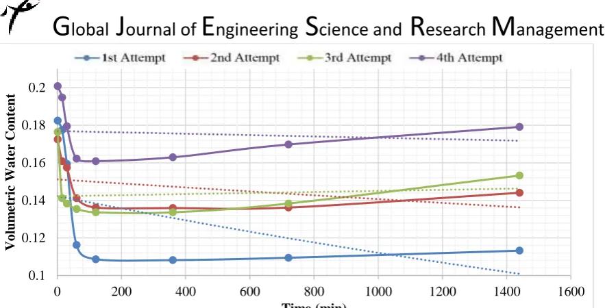
Finally, to show the variation in water content, the four irrigation cycles were grouped for each reflected pipe for the 800 MHz as illustrated in Figures 9 and 10 at the first two pipes. While, Figure 11 shows the relations of the variation in water content during irrigation cycles. The major axis represents the volumetric water content, and the minor axis refers to survey time intervals in minutes. It is obvious from the relations that the volumetric water content for all irrigation cycles and for both the 800 and 500 MHz, show a higher decline during the first double hours after irrigation. This may be due to the pump energy that effects on the water pressure and direction movement during the irrigation, in addition other properties will confidently affect the movement of the water within the model mass (i.e. porosity and void percentage etc.). For this method, in monitoring the water content within the model depending on the hyperbola reflection method, stand for values more regularly when using the 800 MHz rather than the 500 MHz. This may relate that the 500 MHz will give more disturbed reflected hyperbola from the CPVC pipes, i.e. difficult while fitting the hyperbola to the actual location of the pipes, hence, possible errors by the analyst can be encountered, in contrary to the higher frequency.

Figure 9: Grouped relation shows the variation in water content for the irrigation cycles at the first pipe. 0.06 0.08 0.1 0.12 0.14 0.16 0.18 0.2

0 200 400 600 800 1000 1200 1400 1600

[Karim et al., 3(9): September, 2016] ISSN 2349-4506

Impact Factor: 2.785

G

lobal

J

ournal of

E

ngineering

S

cience and

R

esearch

M

anagement

Figure 10: Grouped relation shows the variation in water content for the irrigation cycles at the second pipe. 0.1

0.12 0.14 0.16 0.18 0.2

0 200 400 600 800 1000 1200 1400 1600

Vo

lum

et

ric

Wa

ter

Co

nte

nt

[Karim et al., 3(9): September, 2016] ISSN 2349-4506

Impact Factor: 2.785

G

lobal

J

ournal of

E

ngineering

S

cience and

R

esearch

M

anagement

Figure 11: The variation in water content during irrigation cycles using 800 and 500 MHz.

CONCLUSIONS

In this work, in the light of the intensive implementation of the GPR technique for underlying moisture investigations, the following conclusions can be drawn:

1. Estimation of soil water content using Common-Offset GPR measurements mode facilitates rapid data acquisition.

2. From field data of the three subsurface irrigation pipes, GPR can be used to observe vertical water changes caused by moisture ingress estimated from the two-way travel time of EM waves using the hyperbola reflection method.

3. The dielectric permittivity values are drastically decreased around the irrigation pipes during one irrigation cycle, this can clearly and quantitatively give the vertical extent of the wet area.

4. Promising results were obtained using the Common-offset GPR (800 MHz) with hyperbola method in monitoring the volumetric water under pavement layers. The dielectric constant is strongly dependent on the volumetric water content of the soil. The latter was varied over a range of 8.7% to 20% and about 9.2% to 25.3% using respectively 800 and 500 MHz for the first two pipes.

5. The third buried CPVC pipe was seemed to be difficult to observe at initial irrigation cycles due to the clayey soil, pipe size and its low dielectric constant.

REFERENCES

1. Cassidy N.J., 2009, Electrical and magnetic properties of rocks, soils, and fluids, In: Ground Penetrating Radar: Theory and Applications, Jol, H.M., pp. 41-72, Elsevier, ISBN 978-0-444-53348-7, Amsterdam, The Netherlands.

2. Chen C. and Zhang, J., 2009, “A Review on GPR Applications in Moisture Content Determination and

[Karim et al., 3(9): September, 2016] ISSN 2349-4506

Impact Factor: 2.785

G

lobal

J

ournal of

E

ngineering

S

cience and

R

esearch

M

anagement

3. Davis J.L. and Annan, A.P. 1989, “Ground-penetrating radar for high-resolution mapping of soil and

rock stratigraphy”, Geophysical Prospecting, Vol. 37, 531-551.

4. Evans R., Frost, M., Stonecliffe-jones, M., and Dixon, N., 2007, “Assessment of in Situ Dielectric Constant of Pavement Materials”, Transportation Research Board of the National Academies, Washington, No. 2037, pp. 128-135.

5. Griffin S. and Pippett, T., 2002, “Ground Penetrating Radar”, Geophysical and Remote Sensing Methods

for Regolith Exploration, report 144, pp. 80-89.

6. Hothan J. and Foester M., 2000, “Gültigkeit der mit dem Ground Penetration Radar" (GPR) ermittelten Schichtdicken”, Fachgebiet Konstruktiver Straßenbau, Universität Hannover, (In German).

7. Hubbard, S.S., Rubin Y., and Majer, E., 1997, “Ground-penetrating-radar-assisted saturation and permeability estimation in bimodal systems”, Water Resources Research Vol. 33, pp. 971-990.

8. Huisman J.A., Hubbard S.S., Redman J.D. and Annan, A.P., 2003, “Measuring soil water content with

ground penetrating radar”, Review, Published in Vadose Zone Journal. Soil Science Society of America, Vol. 2, pp. 476-491.

9. Maierhofer C., 2003, “Nondestructive evaluation of concrete infrastructure with ground penetrating radar”, J. Mater. Civ. Eng., Vol. 15, No. 3, pp. 287–297.

10. Saarenketo T., 1997, “Using ground penetrating radar and dielectric probe measurements in pavement

density quality control”, In Transportation Research Record: Journal of the Transportation Research Board No. 1575, TRB, National Research Council, Washington D.C., pp. 34-41.

11. Saarenketo T., and T. Scullion., 2000, “Road Evaluation with Ground-Penetrating Radar”, Journal of Applied Geophysics, Vol. 43, pp. 119–138.

12. Saarenketo T., 2006, “Electrical properties of road materials and subgrade soils and the use of Ground Penetrating Radar in traffic infrastructure surveys”, Ph.D. thesis, Faculty of science, department of Geosciences, University of Oulu.

13. Saito, H., and Kitahara, M., 2012, “Analysis of Changes in Soil Water Content under Subsurface Drip Irrigation Using Ground Penetrating Radar”, Journal of Arid Land Studies, Vol. 22, No. 1, pp. 283 -286. 14. Topp G.C., Davis J.L., Annan A.P., 1980, “Electromagnetic determination of soil water content:

Measurements in coaxial transmission lines”, Water Resources Research Vol.16, pp. 574–582.