Int. J. IndustrialMathematics (ISSN 2008-5621) Vol. 8, No. 3, 2016 Article ID IJIM-00412, 9 pages
Research Article
Generalized H-differentiability for solving second order linear fuzzy
differential equations
P. Darabi∗†, S. Moloudzadeh ‡, H. Khandani§
Received Date: 2013-09-21 Revised Date: 2015-11-09 Accepted Date: 2016-05-22
————————————————————————————————–
Abstract
In this paper, a new approach for solving the second order fuzzy differential equations (FDE) with fuzzy initial value, under strongly generalized H-differentiability is presented. Solving first order fuzzy differential equations by extending 1-cut solution of the original problem and solving fuzzy integro-differential equations has been investigated by some authors (see for example [5,6]), but these methods have been done for fuzzy problems with triangular fuzzy initial value. Therefore by extending the r-cut solutions of the original problem we will obviate this deficiency. The presented idea is based on: if a second order fuzzy differential equation satisfy the Lipschitz condition then the initial value problem has a unique solution on a specific interval, therefore our main purpose is to present a method to find an interval on which the solution is valid.
Keywords: Fuzzy differential equations (FDE); Strongly generalized H-differentiability; r-cut solutions.
—————————————————————————————————–
1
Introduction
T
hhas been rapidly growing in recent years.e topic of fuzzy differential equations (FDE) Kandel and Byatt [20] applied the concept of fuzzy differential equations (FDE) to analyze the fuzzy dynamic problems. The FDE and the initial value problem (Cauchy problem) were treated by Kaleva [21, 22], Seikkala [25], He and Yi [17], Kloeden [23] and some others (see [10,11,12,15,18]). The numerical methods for solving fuzzy differential equations are introduced in [1, 2, 3,4, 7, 9]. Buckley and Feuring [13] in-troduced two analytical methods for solving n-∗Corresponding author. [email protected]
†Department of Mathematics, Farhangian University,
Tehran, Iran.
‡Department of Mathematics, Faculty of Education,
Soran University, Soran/Erbil, Kurdistan Region, Iraq.
§Department of Mathematics, Mahabad Branch,
Is-lamic Azad University, Mahabad, Iran.
order linear differential equations with fuzzy ini-tial value conditions.
A new approach for solving first order fuzzy dif-ferential equations with extending 1-cut solution of original problem is introduced by Allahviran-loo and salahshour [6]. See [5] for a method for fuzzy integro-differential equations with extend-ing o-cut and 1-cut solutions of the original prob-lem, but these methods have been done for fuzzy problems with triangular fuzzy initial value. In this paper by extending r-cut solutions of the original problem we will obviate this deficiency. In [8] we see that, if a second order fuzzy differen-tial equation satisfy the Lipschitz condition, then the initial value problem has a unique solution on a specific interval. The presented method in this paper is an analytical method and with a specific method, we try to find a solution, that the solu-tion is valid. According to the definisolu-tion of gen-eralized derivative, a fuzzy second order differen-tial equation can be transformed to a four-crisp
differential equations. Since the initial differen-tial equations satisfy the Lipschitz condition, the obtained solution is unique. The solutions are obtained from a fuzzy initial value problem. To show that these are fuzzy solutions, we find the intervals in which each solution is a fuzzy solu-tion.
The structure of this paper is organized as follow. In section2, some basic definitions and notations will be given. In section3, second order fuzzy dif-ferential equation is introduced and our method is presented in details. In section4, the proposed method is illustrated by examples. Conclusion is at the end of section5.
2
Basic Definitions and
Nota-tions
In this section, we give some necessary definitions and notations which will be used throughout the paper.
Definition 2.1 Let X be a nonempty set. A fuzzy set u in X is characterized by its member-ship function u :X →[0,1]. Thus u(x) is inter-preted as the degree of membership of an element x in the fuzzy set u for each x∈X.
Let denote by E the class of fuzzy subsets of the real axis (i.e. u:R→[0,1]) satisfying the follow-ing properties:
• u is normal, that is, there existss0 ∈Rsuch
thatu(s0) = 1,
• u is convex fuzzy set (i.e. u(ts+ (1−t)r)≥ min{u(s), u(r)},∀t∈[0,1], s, r∈R),
• u is upper semi-continuous onR,
• cl{s∈R|u(s) >0} is compact, where cl de-notes the closure of a subset.
E is called the space of fuzzy numbers with boundedr-level intervals. This means that if v∈ E then ther-level set
v[r]={s|v(s)≥r},
is a closed bounded interval which is denoted by
v[r]= [v(r), v(r)] for r∈(0,1],
and
v[0] = ∪
r∈(0,1] v[r].
Lemma 2.1 [24] If u, v∈E, then for r ∈(0,1],
(u+v)[r]= [u(r) +v(r), u(r) +v(r)],
(u.v)[r]= [mink,maxk],
where
k={u(r)v(r), u(r)v(r), u(r)v(r), u(r)v(r)}.
Definition 2.2 [19] The Hausdorff distance be-tween fuzzy numbers is given by
D:E×E −→R+∪{0},
D(u, v) = sup
r∈[0,1]
max{|u(r)−v(r)|,|u(r)−v(r)|},
where
u[r]= [u(r), u(r)], v[r]= [v(r), v(r)]⊂E
is utilized.
Then it is easy to see thatDis a metric inE and has the following properties (see[10]).
• D(u⊕w, v⊕w) =D(u, v), ∀u, v, w∈E,
• D(k⊙u, k⊙v) =|k|D(u, v), ∀k∈R, u, v ∈ E,
• D(u ⊕ v, w ⊕ e) ≤ D(u, w) +
D(v, e), ∀u, v, w, e∈E,
• (D, E) is a complete metric space.
Definition 2.3 [10] Let x, y∈E. If there exists z ∈ E such that x = y+z, then z is called the H-difference ofx andy and it is denoted byx⊖y.
Definition 2.4 [10] Let f : (a, b) −→ E and t0 ∈(a, b). We say that f is strongly generalized H-differentiable at t0, if there exists an element f′(t0)∈E, such that:
(1) for all h > 0 sufficiently near to 0, ∃f(t0+ h)⊖f(t0), ∃f(t0)⊖f(t0−h) such that the
following limits hold.
lim
h−→0+
f(t0+h)⊖f(t0) h
= lim
h−→0+
f(t0)⊖f(t0−h) h =f
′
(2) for all h <0 sufficiently near to 0, ∃f(t0)⊖ f(t0+h), ∃f(t0 −h)⊖f(t0) such that the
following limits hold.
lim
h−→0+
f(t0)⊖f(t0+h) h
= lim
h−→0+
f(t0−h)⊖f(t0) h =f
′
(t0). (2.2)
If f(t) is (n)-differentiable at t0, we denote its
first derivatives byD1nf(t0), for n= 1,2.
In the special case whenf is a fuzzy-valued func-tion, we have the following results.
Theorem 2.1 [10] Letf(t)be fuzzy-valued func-tions and denote f(t)[r] = (f(t;r), f(t;r)), for each r∈[0,1]. Then
• if f(t) is (1)-differentiable, then f(t;r) and
f(t;r) have second order derivative and
f′(t)[r]= [f′(t;r), f′(t;r)].
• if f(t) is (2)-differentiable, then f(t;r) and
f(t;r) have second order derivative and
f′(t)[r]= [f′(t;r), f′(t;r)].
Theorem 2.2 [10] let f : (a, b) −→ R and g : (a, b) −→ E be two differentiable functions (g is generalized differentiable as in Definition 2.4).
• If f(t).f′(t) > 0 and g is (1)-differentiable, thenf.g is(1)-differentiable and
(f.g)′(t) =f′(t).g(t) +f(t).g′(t). (2.3)
• If f(t).f′(t) < 0 and g is (2)-differentiable, thenf.g is(2)-differentiable and
(f.g)′(t) =f′(t).g(t) +f(t).g′(t). (2.4)
The main properties of the H-derivatives of first part of the above theorem, some of which still hold for the second part, are well known and can be found in [21] and some other properties of the second part can be found in [14].
Notice that we say fuzzy-valued functionf is (1)-differentiable if satisfy in the first form (1) in Def-inition 2.4. and we say f is (2)-differentiable if satisfy in the second form (2) in Definition2.4.
3
Second Order Fuzzy
Differ-ential Equations
In this section, we are going to investigate a so-lution of fuzzy differential equations (FDE). Consider the following second order fuzzy differ-ential equation:
y′′(t) =f(t, y(t), y′(t)), y(t0) =u0,
y′(t0) =v0,
(3.5)
where f : (a, b)×E ×E −→ E is linear fuzzy-valued function with positive coefficients,u0, v0 ∈ E and the involved derivatives are strongly gen-eralized H-differentiable which is defined in Defi-nition2.4.
Theorem 3.1 [19] Let f(t) and f′(t) are two differentiable fuzzy-valued functions and denote f(t)[r]= [f(t;r), f(t;r)], for eachr ∈[0,1]. Then
• if f(t) and f′(t) are (1)-differentiable, or f(t) and f′(t) are (2)-differentiable, then f(t;r) and f(t;r) have second order and second order derivatives and f′′(t)[r] = [f′′(t;r), f′′(t;r)].
• if f(t) is (1)-differentiable and f′(t) is (2) -differentiable, or f(t) is (2)-differentiable and f′(t) is (1)-differentiable, then f(t;r)
and f(t;r) have second order and sec-ond order derivatives and f′′(t)[r] =
[f′′(t;r), f′′(t;r)].
Definition 3.1 [19] Let f : (a, b) → E and n, m = 1,2. One says fis (n, m)-differentiable at t0 ∈(a, b), if D1nf exists on a neighborhood of
t0 as a fuzzy function and it is (m)-differentiable at t0. The second derivatives of f are denoted by D(2)n,mf(t0) for n, m= 1,2.
Definition 3.2 [19] Let y : (a, b) → E be fuzzy function and n, m ∈ {1,2}. One says that y is an (n, m)-solution for problem (3.5) on (a, b), if Dn1y and D(2)n,my exist on (a, b) and D(2)n,my =
f(t, y(t), D1ny(t)), y(t0) =u0, Dn1ey(t0) =v0.
• If f(t).f′(t) > 0, f′(t).f′′(t) > 0 and g is (1,1)-differentiable, then f.g is (1,1) -differentiable and
(f.g)′′(t)
=f′′(t).g(t)+2f′(t).g′(t)+f(t).g′′(t). (3.6)
• If f(t).f′(t) < 0, f′(t).f′′(t) < 0 and g is (2,2)-differentiable, then f.g is (2,2) -differentiable and
(f.g)′′(t)
=f′′(t).g(t)+2f′(t).g′(t)+f(t).g′′(t). (3.7)
Theorem 3.3 [8] Let f : (a, b) ×E ×E −→ E be continuous, and suppose that there exist M1, M2 >0 such that:
D(f(t, x1, x2), f(t, y1, y2))
≤ M1D(x1, x2) +M2D(x1, x2),
for all t∈(a, b), x1, x2, y1, y2 ∈ E. Then the ini-tial value problem (3.5) has a unique solution on
(a, b) for each case.
Now, we describe our method for solving a FDE (3.5). First, we solve a FDE (3.5) in the sense of r-cut as follows:
Dn,m(2) y[r](t) =f(t, y[r](t), Drny[r](t)),
y[r](t0) =u [r] 0 , Dnry[r](t0) =v[0r],
0≤r≤1, t0 ∈(a, b), n, m= 1,2.
(3.8) Let y[r](t) be an (n, m)-solution for problem (3.8). To find it, based on type of differentiabil-ity we have the following crisp systems, called (n, m)-systems as follows:
(1,1)-system
y′′(t;r) =f(t, y(t;r), y′(t)),
y′′(t;r) =f(t, y(t;r), y′(t;r)),
y(t0;r) =u0(r), y(t0;r) =u0(r),
y′(t0;r) =v0(r), y′(t0;r) =v0(r),
0≤r ≤1.
(3.9)
(1,2)-system
y′′(t;r) =f(t, y(t;r), y′(t;r)),
y′′(t;r) =f(t, y(t;r), y′(t;r)),
y(t0;r) =u0(r), y(t0;r) =u0(r),
y′(t0;r) =v0(r), y′(t0;r) =v0(r),
0≤r ≤1.
(3.10) (2,1)-system
y′′(t;r) =f(t, y(t;r), y′(t;r)),
y′′(t;r) =f(t, y(t;r), y′(t;r)),
y(t0;r) =u0(r), y(t0;r) =u0(r),
y′(t0;r) =v0(r), y
′
(t0;r) =v0(r),
0≤r ≤1.
(3.11) (2,2)-system
y′′(t;r) =f(t, y(t;r), y′(t;r)),
y′′(t;r) =f(t, y(t;r), y′(t;r)),
y(t0;r) =u0(r), y(t0;r) =u0(r),
y′(t0;r) =v0(r), y
′
(t0;r) =v0(r),
0≤r ≤1.
(3.12)
Theorem 3.4 If f is satisfy the Lipschitz con-dition, then there is an interval I that the solu-tion of(n, m)-system is an (n,m)-solution for the problem (3.5) on the interval I.
Proof: Since f satisfy the Lipschitz condition, the initial value problem (3.5) has a unique (n,m)-solution such asy[r]= [y(r), y(r)] on the interval
I ([8]). From the Definition 3.2. and theorems 2.1. and 3.1. y[r] = [y(r), y(r)] is a solution of (n, m)-system. On the other hand, sincef satisfy the Lipschitz condition, then according to [16], the (n, m)-system has a unique solution such as
y∗[r] = [y∗(r), y∗(r)] and it can be shown that
y = y∗. Then y∗ is an (n,m)-solution for the problem (3.5) on the interval I.
of (3.5) be valid on it as fallow:
I = (a, b), b= min{ t| ∃ εi >0 ; yi(t−εi;r)−
yi(t−εi;r) > 0 , yi(t+εi;r)−yi(t+εi;r) <
0 , i= 0,1,2}.
0 0.5
1
−5 0 50 0.5 1
exact solution
0 0.2 0.4 0.6 0.8 1 −4
−2 0 2 4
0−cut solution
0 0.2 0.4 0.6 0.8 1 −2
−1 0 1 2
0−cut solution of first derivative
0 0.2 0.4 0.6 0.8 1 −2
−1 0 1 2
0−cut solution of second derivative
Figure 1.
0 0.5
1
−2 0 20 0.5 1
exact solution
0 0.2 0.4 0.6 0.8 1 −2
−1 0 1 2
0−cut solution
0 0.2 0.4 0.6 0.8 1 −1
−0.5 0 0.5 1
0−cut solution of first derivative
0 0.2 0.4 0.6 0.8 1 −2
−1 0 1 2
0−cut solution of second derivative
Figure 2.
4
Examples
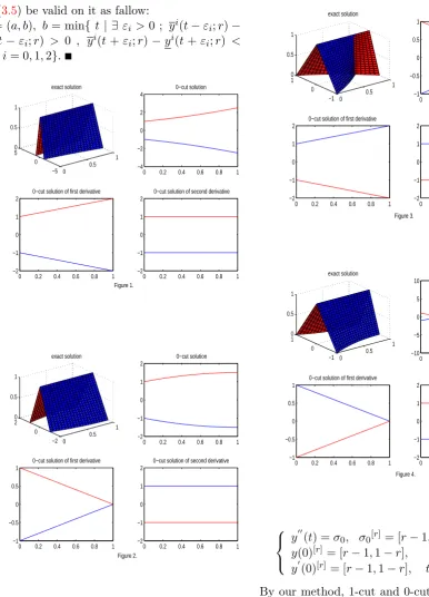
In this section, some examples are given to illus-trate our method and show that our approach is coincide with the exact solutions. Moreover we plot the obtained solutions and derivatives based on the r-cut representation at each case.
Example 4.1 (see [19]) consider the following second order fuzzy differential equation:
0 0.5
1
−1 0 1 0 0.5 1
exact solution
0 0.2 0.4 0.6 0.8 1 −1
−0.5 0 0.5 1
0−cut solution
0 0.2 0.4 0.6 0.8 1 −2
−1 0 1 2
0−cut solution of first derivative
0 0.2 0.4 0.6 0.8 1 −2
−1 0 1 2
0−cut solution of second derivative
Figure 3.
0 0.5
1
−1 0 1 0 0.5 1
exact solution
0 1 2 3 4 5 −10
−5 0 5 10
0−cut solution
0 0.2 0.4 0.6 0.8 1 −1
−0.5 0 0.5 1
0−cut solution of first derivative
0 0.2 0.4 0.6 0.8 1 −2
−1 0 1 2
0−cut solution of second derivative
Figure 4.
y′′(t) =σ0, σ0[r]= [r−1,1−r], y(0)[r]= [r−1,1−r],
y′(0)[r]= [r−1,1−r], t≥0.
(4.13)
By our method, 1-cut and 0-cut systems are de-rived as follows respectively:
Case(I): Suppose that y(t) and y′(t) are (1)-differentiable functions. By solving ODE (3.9) we get:
y(t;r) = (r−1)(t
2
2 +t+ 1),
y(t;r) = (1−r)(t
2
2 +t+ 1),
and
y(t)[r]= [r−1,1−r](t
2
0
0.5 1 −5
0 5 0 0.5 1
exact solution
0 0.5 1
−2 0 2 4 6
0−cut solution
0 0.5 1
−2 0 2 4
0−cut solution of first derivative
0 0.5 1
−2 0 2 4 6
0−cut solution of second derivative
Figure 5.
0 0.5 1
−5 0 5 0 0.5 1
exact solution
0 0.5 1
−1 0 1 2 3
0−cut solution
0 0.5 1
−1 0 1 2
0−cut solution of first derivative
0 0.5 1
−1 0 1 2 3
0−cut solution of second derivative
Figure 6.
by drawing the 0-cut solutions of the first and second derivatives we see thaty(t) has valid level sets for t ≥ 0 and y′(t) has valid level sets for
t≥0 and alsoy′′(t) has valid level sets fort≥0, then by intersection of these valid level sets we get y(t) that is a (1,1)-solution for the original problem on [0,+∞). (See Figure1).
Case(II): Let y(t) be a (1)-differentiable function and y′(t) be a (2)-differentiable func-tion. By solving ODE (3.10) , we get:
y(t;r) = (r−1)(−t
2
2 +t+ 1),
y(t;r) = (1−r)(−t
2
2 +t+ 1),
0
0.5 1 0
1 2 0 0.5 1
exact solution
0 0.5 1
0 0.5 1 1.5 2
0−cut solution
0 0.5 1
−1 0 1 2 3
0−cut solution of first derivative
0 0.5 1
0 0.5 1 1.5 2
0−cut solution of second derivative
Figure 7.
0 0.5 1
0 1 2 0 0.5 1
exact solution
0 1 2 3
0 5 10 15 20
0−cut solution
0 1 2 3
−10 0 10 20
0−cut solution of first derivative
0 1 2 3
0 5 10 15 20
0−cut solution of second derivative
Figure 8.
and
y(t)[r]= [r−1,1−r](−t
2
2 +t+ 1),
by drawing the 0-cut solutions of the first and second derivatives we see thaty(t) has valid level sets for t ≥ 0 and y′(t) has valid level sets for 0 ≤ t ≤ 1 and also y′′(t) has valid level sets for
t ≥ 0, then by intersection of these valid level sets we get y(t) that is a (1,2)-solution for the original problem on [0,1]. (See Figure2).
Case(III): Let y(t) be a (2)-differentiable function and y′(t) be a (1)-differentiable func-tion. By solving ODE (3.11) we get:
y(t;r) = (r−1)(−t
2
y(t;r) = (1−r)(−t
2
2 −t+ 1),
and
y(t)[r]= [r−1,1−r](−t
2
2 −t+ 1),
by drawing the 0-cut solutions of the first and second derivatives we see thaty(t) has valid level sets for 0 ≤t ≤√3−1 andy′(t) has valid level sets for t ≥ 0 and also y′′(t) has valid level sets fort≥0, then by intersection of these valid level sets we get y(t) that is a (2,1)-solution for the original problem on [0,√3−1]. (See Figure 3).
Case(IV): Suppose that y(t) and y′(t) are (2)-differentiable functions. By solving ODE (3.12), we get:
y(t;r) = (r−1)(t
2
2 −t+ 1),
y(t;r) = (1−r)(t
2
2 −t+ 1),
and
y(t)[r]= [r−1,1−r](t
2
2 −t+ 1),
by drawing the 0-cut solutions of the first and second derivatives we see thaty(t) has valid level sets for t ≥ 0 and y′(t) has valid level sets for 0 ≤ t ≤1 and also y′′(t) has valid level sets for
t ≥ 0 , then by intersection of these valid level sets we get y(t) that is a (2,2)-solution for the original problem on [0,1]. (See Figure4).
Using 1-cut and 0-cut solutions we show that the discussed method can be applied to solve the fuzzy differential equations.
Example 4.2 Let us consider the following sec-ond order FDE:
y′′(t) =y(t),
y(0)[r]= [r2,2−r2],
y′(0)[r]= [r2−1,1−r2] t≥0.
(4.14)
Based on the proposed approach, 1-cut and 0-cut systems are derived as follows respectively:
Case(I):
Suppose that y(t) and y′(t) are (1)-differentiable functions. By solving ODE (3.9), we get:
y(t;r) = 1 2e
−t+et(r2−1/2),
y(t;r) = 1 2e
−t−et(r2−3/2),
by drawing the 0-cut solutions of the first and second derivatives we see thaty(t) has valid level sets for t ≥ 0 and y′(t) has valid level sets for
t≥0 and also y′′(t) has valid level sets for t≥0 , then by intersection of these valid level sets we get y(t) that is a (1,1)-solution for the original problem on [0,+∞). (See Figure5).
Case(II):
Lety(t) be a (1)-differentiable function and y′(t) be a (2)-differentiable function. By solving ODE (3.10) , we get:
y(t;r) =cosh(t) + 2r.sinh(log(r)).sin(t) + 2r.sinh(log(r)).cos(t),
y(t;r) =cosh(t)−2r.sinh(log(r)).sin(t) −2r.sinh(log(r)).cos(t),
by drawing the 0-cut solutions of the first and second derivatives we see thaty(t) has valid level sets for t ≥ 0 and y′(t) has valid level sets for 0 ≤ t ≤ π4 and also y′′(t) has valid level sets for
t ≥ 0, then by intersection of these valid level sets we get y(t) that is a (1,2)-solution for the original problem on [0,π4]. (See Figure 6).
Case(III):
Lety(t) be a (2)-differentiable function and y′(t) be a (1)-differentiable function. By solving ODE (3.11), we get:
y(t;r) =cosh(t)−2r.sinh(log(r)).sin(t) + 2r.sinh(log(r)).cos(t),
y(t;r) =r.cosh(t) + 2r.sinh(log(r)).sin(t) −2r.sinh(log(r)).cos(t),
the original problem on [0,π4].(See Figure7).
Case(IV):
Suppose that y(t) and y′(t) are (2)-differentiable functions. By solving ODE (3.12) , we get:
y(t;r) = 1 2e
t+ (r2−1/2)e−t,
y(t;r) = 1 2e
t−(r2−3/2)e−t,
by drawing the 0-cut solutions of the first and second derivatives we see thaty(t) has valid level sets for t ≥ 0 and y′(t) has valid level sets for
t≥0 and alsoy′′(t) has valid level sets fort≥0, then by intersection of these valid level sets we get y(t) that is a (2,2)-solution for the original problem on [0,+∞). (See Figure8).
5
Conclusions
In this paper a new approach for solving sec-ond order fuzzy differential equations (FDE) with fuzzy initial value under strongly generalized H-differentiability is considered. The presented idea is based on: if a second order fuzzy differential equation satisfy the Lipschitz condition then the initial value problem has a unique solution on a specific interval. We obtain this solution by trans-forming the fuzzy initial value of the generalized derivatives to the four-crisp differential equations and then solve them. Using solutions of the first and second derivatives we choose an interval such that the differential equations’s solution is valid on it.
References
[1] S. Abbasbandy, T. Allahviranloo, P. Darabi,
Numerical solution of n-th order fuzzy dif-ferential equations by Runge-Kutta method, Mathematical and Computtational Applica-tions 16 (2011) 935-946.
[2] S. Abbasbandy, T. Allahviranloo, P. Darabi, O. Sedaghatfar,Variational iteration method for solvingn-th order fuzzy differential equa-tions, Mathematical and Computtational Applications 16 (2011) 819-829.
[3] S. Abbasbandy, T. Allahviranloo, Oscar´ L´opez-Pouso, J. J. Nieto, Numerical Meth-ods for Fuzzy Differential Inclusions, Com-put. Math. Appl. 48 (2004) 1633-1641.
[4] S. Abbasbandy, T. Allahviranloo, Numeri-cal solutions of fuzzy differential equations by taylor method, Comput. Methods Appl. Math. 2 (2002) 113-124.
[5] T. Allahviranloo, S. Abbasbandy, O. Sedaghatfar, P. Darabi, A New Method for Solving Fuzzy Integro-Differential Equation Under Generalized Differentiability, Neural Computing and Applications 21 (2012) 191-196.
[6] T. Allahviranloo, S. salahshour, A new ap-proach for solving first order fuzzy differen-tial equations, IPMU. (2010) 522-531.
[7] T. Allahviranloo, N. Ahmady, E. Ahmady,
A method for solving n-th order fuzzy linear differential equations, Comput. Math. Appl. 86 (2009) 730-742.
[8] T. Allahviranloo, N. A, Kiani, M. Barkhor-dari, Toward the exiistence and uniqueness of solution of second-order fuzzy differential equations, Information Sciences 179 (2009) 1207-1215.
[9] T. Allahviranloo, N. Ahmady, E. Ahmady,
Numerical solution of fuzzy differential equa-tions by predictor-corrector method, Infor. Sci. 177 (2007) 1633-1647.
[10] B. Bede, I. J. Rudas, A. L. Bencsik,First or-der linear fuzzy differential equations unor-der generalized differentiability, Inform. Sci. 177 (2007) 1648-1662.
[11] J. J. Buckley, T. Feuring, Fuzzy differen-tial equations, Fuzzy sets and Systems 110 (2000) 43-54.
[12] J. J. Buckley, T. Feuring, Introduction to fuzzy partial differential equations, Fuzzy Sets and Systems 105 (1999) 241-248.
[14] Y. Chalco-cano, H. Roman-Flores, On new solutions of fuzzy differential equations
Chaos, Solitons and Fractals 38 (2006) 112-119
[15] W. Congxin, S. Shiji, Existence theorem to the Cauchy problem of fuzzy differen-tial equations under compactness-type condi-tions, Infor. Sci. 108 (1998) 123-134.
[16] C. W. Gear, Numerical Initial Value Prob-lem In Ordinary, Differential Equations (1971).
[17] O. He, W. Yi, On fuzzy differential equa-tions, Fuzzy Sets and Systems 24 (1989) 321-325.
[18] L. J. Jowers, J. J. Buckley, K. D. Reilly, Sim-ulating continuous fuzzy systems, Infor. Sci. 177 (2007) 436-448.
[19] A. Khastan, F. Bahrami, K. Ivaz, New results on multiple solutions for Nth-order fuzzy differential Under Generalized Dif-ferentiability, Boundary Value Problems 2009, http://dx.doi.org/10.1155/2009/ 395714/.
[20] A. Kandel, W. J. Byatt, Fuzzy differen-tial equations, Proceedings of the Interna-tional Conference on Cybernetics and Soci-ety, Tokyo (1978) 1213-12160.
[21] O. Kaleva, Fuzzy differential equations, Fuzzy Sets and Systems 24 (1987) 301-317.
[22] O. Kaleva,The Cauchy problem for fuzzy dif-ferential equations, Fuzzy Sets and Systems 35 (1990) 389-396.
[23] P. Kloeden,Remarks on peano-like theorems for fuzzy differential equations, Fuzzy Sets and Systems 44 (1991) 161-164.
[24] D. Ralescu, A survey of the representation of fuzzy concepts and its applications, in: M. M. Gupta, R. K. Ragade, R. R. Yager, Eds., Advances in Fuzzy Set Theory and Appli-cations (North-Holland, Amsterdam (1979) 77-91.
[25] S. Seikkala, On the fuzzy initial value prob-lem, Fuzzy Sets and Systems 24 (1987) 319-330.
Pejman Darabi was born in
Tehran-Iran in 1978. He received B.Sc and M.Sc degrees in ap-plied mathematics from Sabzevar Teacher Education University, Science and Research Branch, IAU to Tehran, respectively, and his Ph.D degree in applied mathematics from science and research Branch, IAU, Tehran, Iran in 2011. Main research interest include numerical solution of Fuzzy differential equation systems, ordinary differential equation, partial differential equation, fuzzy linear system and similar topics.
Saeid Moloudzadeh was born in the Naghadeh-Iran in 1976. He re-ceived B.Sc degree in mathematics and M.Sc degree in applied mathe-matics from Payam-e-Noor Univer-sity of Naghadeh, Science and Re-search Branch, IAU to Tehran, re-spectively, and his Ph.D degree in applied math-ematics from Science and Research Branch, IAU, Tehran, Iran in 2011. He is research interests in-clude fuzzy mathematics, especially, on numerical solution of fuzzy linear systems, fuzzy differential equations and similar topics.