325
Interaction Vortex – Boundary Layer :
Numerical study of wall mechanisms
S. Pellerin* and A. Giovannini
*
LIMSI-CNRS, UPR 3251, BP 133, F-91403 Orsay Cedex, France, [email protected]
Institut de Mécanique des Fluides de Toulouse, UMR 5502 CNRS/INP-UPS, Université Paul Sabatier, 118 Route de Narbonne, F-31062 Toulouse Cedex, France, [email protected]
Abstract
The interactions between a coherent vortex structure and a flat plate boundary layer are investigated. The unsteady numerical method used associates the Vortex-In-Cell algorithm for the convection step to the Random Walk algorithm for the diffusion one. The boundary layer is discretized by a large number of vortices, 105
. An appropriate choice of discretization parameters leads to a good solution for the flat plate and exhibits a minimal numerical dissipation. Interactions are studied for different Reynolds numbers, for positive and negative vortices. The Lighthill’s mechanism of production of vorticity is observed. In the case of a negative vortex, a recirculation zone appears and a secondary structure with positive vorticity is created inside the boundary layer. The ejection of this structure induces the rebound of the main vortex. The wall mechanisms, particularly the study of Cf and Cp evolutions, confirm previous behaviors.
Introduction
The interactions between vortical structures and boundary layers can be observed in many industrial flows, as turbomachines or helicopters rotors. It may concerns the interactions of wakes, vortices due to incidence variations on blades or marginal tip vortices. They can induce boundary layer separation, decrease of performances, noise and vibrations and strong heat and mass transfers. In order to manage those phenomena, it is necessary to gather information on flow variables in the vicinity of the wall.
Harvey and Perry [8] were the first to study the problem with marginal trailing vortices. They conducted an experiment and explained the main mechanisms for an interaction with a negative vortex. A negative vortex induces an adverse pressure gradient and then a separation in the boundary layer associated to a bubble of recirculation. This bubble grows and detaches itself from the solid wall. It becomes a secondary structure. Doligalski and Walker [5] proposed analytical solutions for an inviscid flow. They proved the existence of a recirculation zone in the case of a negative vortex strong enough.
The aim of this work is the study of dynamic phenomena observed when a coherent structure, a Rankine vortex, is convected in proximity of a solid wall. A recent review concerning the interactions was realized by Doligalski et al. [4]. Interactions for vortices with negative and positive circulations, so with clockwise and counter-clockwise rotations, are investigated. The influence of the interaction at the wall, particularly through the stress tensor components, is studied.
I. Numerical method
I.1 A mixed eulerian-lagrangian method
Many incompressible flows are characterized by compact rotational regions. The vortex methods simulate such flows by discretizing the zones of concentrated vorticity with vortical particles and displacing them by a lagrangian technique [1]. These methods have the advantage that they concentrate the computational effort on rotational zones. In addition, they minimize the numerical dissipation encountered with the approximations of space and time derivative terms [7]. The vortex methods are particularly adapted to the simulation of bidimensional, uncompressible and unsteady flows, with predominating convective effects. In 2-D flows, these methods use the non-zero component of the curl of the velocity, the vorticity ω, as the transport variable. The Navier-Stokes equations are reformulated introducing vorticity, as:
( )
ω
∂
ω
∂
1
.
u
t
e∆
ℜ
=
∇
+
&
, (1)where ℜe is the Reynolds number of the flow and
u
the velocity vector. Optimal boundary conditions areused (section I.2). The equation (1) is solved by splitting it into convection and diffusion operators, both equations being treated separately:
( )
ω
∂
ω
∂
=
∇
.
u
t
&
, (2.a)ω
∂
ω
∂
1
t
e∆
ℜ
=
. (2.b)The vorticity field is discretized into a finite number of vortices nv. For a given time step, the total
displacement is obtained by adding convective and diffusive movements:
(
x,
y,
t
+
dt
)
iℵ
=ℵ
i(
x,
y,
t
)
+L
(
u
i(
ℵ
i(
x,
y,
t
)
,
t
)
,
dt
)
+η
. (3)The diffusion step is treated by the Random Walk algorithm [1]. The diffusive transport
η
is then simulated from a random process and a gaussian distribution obtained from the bidimensional Green solution of equation (2.b). The convective step is treated by the Vortex-In-Cell algorithm, introducing an eulerian grid.L
represents the integration operator for the velocity field. The VIC algorithm, proposed by Christiansen [2], associates an eulerian grid to the initial lagrangian formulation. A Poisson equation for the stream-function Ψ is solved over this grid:∆ Ψ = − ω. (4)
For each vortex, the circulation is discretized on a grid with the method of weighted surfaces. The Poisson equation is solved and the velocities on the mesh are obtained from values of the stream-function. The vortex velocities are computed by interpolations between the velocities over the grid, allowing then a lagrangian transport of vortex particles. Globally, the total computational time is mainly proportional to the number of vortices nv.
I.2 Initial and boundary conditions
A flat plate geometry is considered. The initial condition corresponds to the potential solution. The boundary conditions are no-slip at the wall and exact solutions at both inlet and upper boundaries. Those conditions use the complex potential theory, which consider the influence of the discretized vorticity field [14]. The influences if each vortex and its image may be estimated using the theory of the hydrodynamic image:
Inlet:
( )
(
[
(
i) (
2 i)
2]
[
(
i) (
2 i)
2]
)
n 1 i i
y
y
x
x
ln
y
y
x
x
ln
L
U
4
y
y
,
x
v−
+
−
−
+
+
−
+
=
∑
=
π
∞Γ
Ψ
(5.a)Top:
y
∂
∂Ψ
( )
(
) (
)
(
) (
)
−
+
−
−
−
+
+
−
+
+
=
=
∑
= ∞ i 2
2 i i 2 i 2 i i n 1 i i x
y
y
x
x
y
y
y
y
x
x
y
y
L
U
2
1
y
,
x
u
vπ
Γ
(5.b)This improvement has the advantage to be accurate when a coherent vortex is introduced into the domain close to the boundaries, to simulate the interaction phenomenon.
The no-slip boundary condition is enforced and induces a generation of vorticity [10]. For a wall element of length δs, an appropriate amount of circulation δΓ is generated in order to cancel the slip velocity Uslip on the wall, a spurious slip velocity [9]:
The wall is discretized with small rectilinear elements. This operation is applied to each element, which is characterized by a local slip velocity and a corresponding circulation Γwall,i. The no-slip condition
introduces a discretization parameter, Γunit, the elementary circulation of vortices. For a given segment i, the
circulation Γwall,i is discretized onto a finite number of vortex particles, ni, function of Γunit:
ni = Int
+
0
.
5
unit i , wall
Γ
Γ
(7)
ni is the closer integer of the ratio of |Γwall,i| /Γunit. Each vortex has a positive or negative circulation Γi
which depends on Γwall,i, so on the sign of the local slip velocity:
i i , wall i
n
Γ
Γ =
(8)II. Numerical results
II.1 Validation of the numerical method
A flat plate boundary layer is modeled for a Reynolds number ℜeL = 104, which leads to a boundary layer
thickness δ ≈ 0.5 at the exit of the domain. The Reynolds number ℜeL is based on both the length of the
plate L and the flow velocity U∞. The results are compared with Blasius’s solution for the flat plate and computer resources are considered. This study leads to a choice of discretization parameters, particularly the elementary circulation Γunit [14 and 15]. The grid chosen corresponds then to 100 (nx) × 50 (ny), for a
domain size of 10 × 2 and refined at the wall and at the inlet of the domain. The time step is equal to 10-2. When Γunit decreases, the number of vortices which discretizes the boundary layer increases (equation
7). The solution is then more accurate but computational time and storage increase considerably. The value
Γunit = 10-4 represents a good compromise between computer resources and quality of results. The boundary
layer is then discretized by nv≈ 2 × 10 5
vortices. The differences between two types of boundary conditions are shown on figure 1, for the normal velocity profiles uy. For uniform conditions the velocity increases out
of the boundary layer. For exact conditions with the complex potential theory, the influence of the boundary layer on frontiers is considered and then the profiles have a coherent behavior. Inside the boundary layer, the solution is in good agreement with Blasius solution.
II.1 Interactions vortex - boundary layer
Interactions between a coherent vortex, the Rankine one, and the flat plate boundary layer previously established, are simulated (figure 2). The characteristic parameter of the phenomenon is the reduced circulation γ, based on the velocity field U∞, the vortex circulation ΓR and the initial distance from the wall
h:
h
U
4
R
∞
=
π
Γ
γ
. Initially, a discretized Rankine vortex is introduced in the domain at (x0,y0) = (2,1), so ath = 1 from the solid wall, for a grid 100 × 150 adapted to a domain size of 10 × 4. The results presented concern three values of the reduced circulation γ. The interactions studied are classified in weak, |γ| = 0.05, moderate, |γ| = 0.15 and strong, |γ| = 0.4.
the fluid particle and the vortex, assimilated to point structures, can be studied. Two opposite sign structures have parallel trajectories in the upward direction. So, a positive vortex moves up from the wall. In the negative case, two identical sign structures turn around each other. So, the negative vortex can stay at a equivalent distance from the wall.
II.2 Time evolution of the interaction
Vorticity and stream function fields permit to follow the time evolution of the phenomenon. Strong interactions are firstly presented (|γ| = 0.4), for the lowest Reynolds number ℜeL = 103. In a case of a
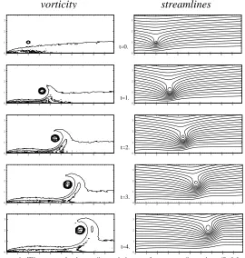
positive vortex (figure 4), the boundary layer lifts up downstream of the vortex. The vortex can be followed on the streamlines. There is no recirculation zone. The vortex moves up from the wall as it is shown on the trajectories in section II.3.
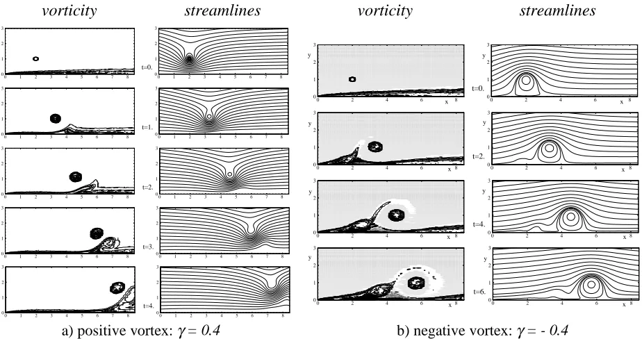
For a negative vortex (figure 5), the rolling around the vortex, upstream, concerns a large part of the boundary layer. In comparison with the positive case, the phenomenon is stronger, because of the velocity flow influence. The vortex is stopped in its movement by the interaction. The convection velocity of the vortex, Vc, can be written as: Vc = U∞ (1+γ). Thus, a negative vortex moves slower than a positive one. The
vortex induces an adverse pressure gradient and a separation inside the boundary layer. A bubble of recirculation with opposite sign circulation is then created. This bubble is visible for lower interactions. In this case, it is immediately absorbed by the global rotation movement. You can see on streamlines the main recirculation zone around the vortex. When the vortex is introduced in the domain, the boundary layer generates an appropriate amount of positive circulation. A zone with positive vorticity is then created at the wall (in dark on figure 5). This zone grows and becomes a secondary structure, ejected out of the boundary layer. This structure interacts with the main vortex and induces its rebound (section II.3).
For higher Reynolds numbers, ℜeL = 10 4
and ℜeL = 10 5
, the boundary layer is thinner and the vorticity more concentrated. The convective effects are stronger in comparison with the diffusion ones. In the positive case, for ℜeL = 10
4
(figure 6.a), the boundary layer doesn’t have the time to form a plume as in the precedent case. The vortex goes faster and impacts on the boundary layer. The boundary layer forms then a patch of vorticity downstream. In addition, the vortex seems to lift up from the wall less rapidly. For a negative vortex (figure 6.b), the main recirculation is an obstacle for the flow which impacts on it. The boundary layer forms a resident vorticity zone upstream the recirculation. The blockage effect of the boundary layer induces a second recirculation bubble above it. This second zone is clearly observed on streamlines. In this case, the positive secondary structure is moderate and the rebound is low.
For
ℜeL = 10 5, the vortex is too far away from the boundary layer and the interaction is very low. In this configuration (h=1), we can't observe the rebound and the creation of the positive structure. The results obtained for the vortex trajectory are only considered.
II.3 Vortex trajectory
The trajectories of the vorticity center of the discretized Rankine vortex are investigated for the different interactions. The vorticity center is defined from the second invariant
I
1. The vectorI
1 , the first momentof vorticity, locates the center of vorticity rc = (xc,yc) =
I
1I
0, where I0 represents the total circulation. Formoderate interactions (|γ| = 0.15, figure 7.a), for every Reynolds number, the vortex has upward trajectory in the case of a positive circulation and downward trajectory in the case of a negative one. When the Reynolds number increases, the vortex moves slowly upward. In addition, the stronger is the circulation, the higher is the trajectory.
upward trajectory, which leads to a rebound for the main vortex. For ℜeL = 104, the rebound occurs later
both in time and in space because the ejection of the secondary structure becomes later.
The complex phenomenon of rebound has been described in several studies. Orlandi (1990) investigated numerically the interaction between a vortex dipole and a flat plate boundary layer, for a vertical impact on a wall.
II.4 Stress tensor components
The wall stress tensor behavior is studied in order to characterize the wall mechanisms due to the interaction. The shear stress coefficient Cf is computed from the longitudinal velocity distribution at the
wall proximity:
Cf =
wall x e
y
u
2
∂
∂
ℜ
(9)The wall shear stress coefficient is compared to the Blasius solution for the flat plate. The figures 8 and 9 represent Cf evolutions at different times, for ℜeL = 10
3
and 104, for an interaction with a negative vortex. Far from the interaction, the solution is in agreement with the Blasius evolution for the flat plate. A recirculation zone corresponds to negative Cf values. The main recirculation zone is identified (figures 8
and 9), and also the secondary recirculation bubble (figure 9). The rebound of the vortex appears more clearly in the first case (figure 8) than in the second (figure 9). When the vortex bounds, its influence at the wall decreases and then the Cf values too. This behavior emphasizes the fact that the secondary positive
structure is stronger for ℜeL = 10 3
.
The study of the wall pressure coefficient Cp permits to enlighten the Lighthill’s mechanism of vorticity
production [10]. In 2-D flow, the vorticity flux
φ
is reduced to its normal component φz (for a (xOy)representation): wall
∂
∂
=
y
-z
ω
ν
φ
(10)For an incompressible viscous flow, the vorticity flux is directly proportional to the pressure gradient [9]:
y
x
p
wall wall1
∂
∂
=
∂
∂
ν
ω
ρ
(11)In our study, the vortex induces an adverse pressure gradient and then a vorticity flux at the wall.
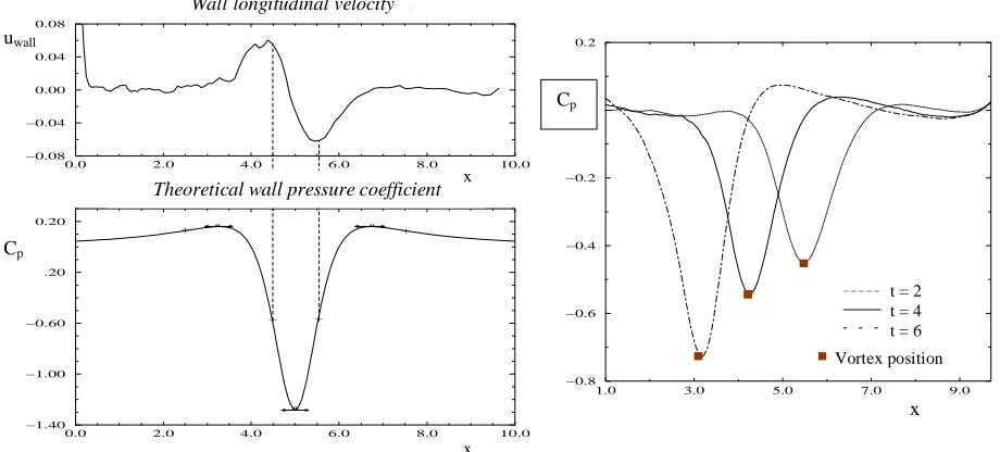
The figure 10 represents the velocity at the wall after the convection step and the theoretical pressure distribution. When the pressure gradient is positive, the vorticity flux has the same sign. The vortex creation algorithm creates, with the no-slip condition (equation 6), an amount of opposite circulation, over the time
δt and a wall segment δs, to cancel the spurious velocity: δΓ
=
φ
zδ
t
δ
s = - U
slipδ
s
. In this case, thespurious slip velocity is negative. Inversely, when the pressure gradient is negative, there is a positive velocity at the wall. The vorticity creation correspond to the passage of the vortex and it is mainly due through the pressure gradient to unsteady effects.
The wall pressure coefficient is obtained from analytical expressions using potential theory:
( )
∑
=
+
−
−
=
ntot1 k k k k k 2 p
dt
dy
y
dt
dx
x
2
u
1
y
,
x
C
∂
Φ
∂
∂
Φ
∂
(12)ntot represents the sum of the nv boundary layer vortices and the nr discretized Rankine vortices. Φ, the
velocity potential, is given by:
−
+
−
−
−
+
=
∑
= ∞ k
k k k n 1 k k
x
x
y
y
tan
Arc
x
x
y
y
tan
Arc
L
U
2
x
totπ
Γ
The following expressions are obtained for uk and vk velocities:
(
) (
)
(
) (
)
− + − − − + + − + + + = =∑
≠ = ∞∞ k l 2
2 l k l k 2 l k 2 l k l k n k l 1 l l k k k k y y x x y y y y x x y y L U 2 L U y 4 1 dt dx u tot π Γ π
Γ (14.a)
(
) (
)
(
) (
)
− + − − − + + − − − = =∑
≠= ∞ k l 2
2 l k l k 2 l k 2 l k l k n k l 1 l l k k y y x x x x y y x x x x L U 2 dt dy v tot π
Γ (14.b)
The number of total vortices ntot being so large (2 × 10 5
), the circulation of every vortex is splitted over a grid, in order to reduce the computational time. The pressure evolution, smoothed on figure 11, is coherent with respect to the theory and the rebound is also observed in the case of a strong negative interaction. Luton et al. (1995) studied the phenomenon of interactions for an Oseen vortex with a fractional-step method. These authors presented also preliminary comments on Cf and Cp evolutions.
Conclusion
This work is devoted to interactions between a coherent structure and a flat plate boundary layer. This simple academic case leads to a better understanding about interaction mechanisms. A parametric study of this complex phenomenon is investigated. Interactions have been simulated for three Reynolds number,
ℜeL = 10 3
, 104 and 105, and three values of vortex circulation, in negative and positive cases. The pressure gradient induced by the vortex convection generates, through the Lighthill’s mechanism, a vorticity flux at the wall during the interaction. Inside the boundary layer, according to the sign of the vortex, a rolling phenomenon is observed, with an effect of wave upstream or downstream. The vortex has upward or downward trajectory depending on its sign. For a strong negative vortex, a recirculation zone and a bubble of vorticity are created. A secondary structure is then generated, with opposite vorticity, and ejected out of the boundary layer. The vortex then bounds.
Perspectives of this work are firstly an extension to multipole vortex structures with different size and intensities. An other complementary work can be the impact situation in which the initial trajectory is normal to the wall.
References
1 CHORIN, A.J., Numerical study of slightly viscous flow. J. Fluid Mech. 57 (1973), 785--796.
2 CHRISTIANSEN, J.P.: Numerical simulation of hydrodynamics par the method of point vortices. J. Comp. Phys. 13 (1973), 363--379.
3 DEE, F.S. and NICHOLAS, O.P.: Flight measurements of wing tip vortex motion near the ground. British Aeronautical Research Council, London, England CP 1065 (1968).
4 DOLIGALSKI, T.L., SMITH, C.R. and WALKER, J.D.A.: Vortex interactions with walls. Ann. Rev. Fluid Mech. 26 (1994), 573--616.
5 DOLIGALSKI, T.L. and WALKER, J.D.A.: The boundary layer induced by a convected two-dimensional vortex. J. Fluid Mech. 139 (1984), 1--28.
6 GAGNON Y., GIOVANNINI, A. and HÉBRARD P.: Numerical simulations and physical analysis of high Reynolds number recirculating flows behind sudden expansions. Phys. Fluids A 5 (10) (1993), 2377--2389.
8 HARVEY, J.K. and PERRY, F.J.: Flowfield produced by trailing vortices in the vicinity of the ground. AIAA Journal 9 (8) (1971), 1659--1660.
9 KOUMOUTSAKOS, P.: Active control of vortex-wall interactions. Phys. Fluids 9 (12) (1997), 3808--3816.
10 LIGHTHILL, E.: Laminar boundary layer theory. ed. Rosenhead L., Oxford University Press, England (1963).
11 LUTON, A., RAGAB, S. and TELIONIS, D.: Interactions of spanwise vortices with a boundary layer. Phys. Fluids 7 (11) (1995), 2757--2765.
12 ORLANDI, P.: Interaction of spanwise vortices with a boundary layer. Phys. Fluids A 2 (8) (1990), 1429--1436.
13 PEACE, A.J. and RILEY, N.: A viscous vortex pair in ground effect, J. Fluid Mech. 129 (1983), 409--426.
14 PELLERIN, S.: Interactions d’une structure tourbillonnaire avec une couche limite de plaque plane: analyse et caractérisation des phénomènes aérodynamiques. PhD thesis, Université Paul Sabatier, Toulouse, 9 january 1997.
15 PELLERIN, S. and GIOVANNINI, A.: Interactions dynamiques entre un tourbillon de type Rankine et une couche limite de plaque plane. C. R. Acad. Sci. Paris Série II b 322 (1996) 793--800.
16 PELLERIN, S. and GIOVANNINI, A.: Analyse physique de l'interaction forte d'une structure tourbillonnaire avec une couche limite. 13e Congrès Français de Mécanique, Poitiers-Futuroscope, France, 1-5 september 1997.
17 STRAUS, J., RENZONI, P. and MAYLE, R.E.: Airfoil pressure measurements during a blade-vortex interaction and a comparison with theory. AIAA Journal 28 (2) (1990), 222--228.
Figure 1: Normal velocity profiles for ℜeL = 10 3
. Figure 2: Interaction vortex – boundary layer.
Figure 3: Influences and trajectories for positive and negative vortices.
vorticity
streamlines
Figure 4: Time evolution of vorticity and stream-function fields; strong interaction with a positive vortex γ = 0.4, for ℜeL = 10
3
.
positive vortex negative vortex
U
∞U
∞0 1 2 3 4 5 6 7 8 9 0
1 2 3
0 1 2 3 4 5 6 7 8 9 0
1 2 3
0 1 2 3 4 5 6 7 8 9 0
1 2 3
0 1 2 3 4 5 6 7 8 9 0
1 2 3
0 1 2 3 4 5 6 7 8 9 0
1 2 3
0 1 2 3 4 5 6 7 8 9 0
1 2 3
t=0.
0 1 2 3 4 5 6 7 8 9 0
1 2 3
t=1.
0 1 2 3 4 5 6 7 8 9 0
1 2 3
t=2.
0 1 2 3 4 5 6 7 8 9 0
1 2 3
t=3.
0 1 2 3 4 5 6 7 8 9 0
1 2 3
t=4.
vortex
y
x
U∞
boundary layer
flat plate
h
ΓR
0.0 2.0 4.0 6.0 8.0 10.0
0.0 0.5 1.0 1.5 2.0
0.0 2.0 4.0 6.0 8.0 10.0
0.0 0.5 1.0 1.5 2.0
Blasius’s solution Numerical results
x y
y
Exact boundary conditions
x
Uniform boundary conditions v=1/15 Uniform boundary conditions
Exact boundary conditions
Blasius’s solution Numerical results
vorticity
streamlines
Figure 5: Time evolution of vorticity and stream-function fields; strong interaction with a negative vortex
γ = - 0.4, for ℜeL = 10 3
. Secondary positive structure (in dark).
vorticity
streamlines
vorticity
streamlines
a) positive vortex: γ = 0.4 b) negative vortex: γ = - 0.4
Figure 6: Vorticity and stream-function fields; strong interaction for ℜeL = 10 4
0 1 2 3 4 5 6 7 8
0 1 2 3
0 1 2 3 4 5 6 7 8
0 1 2 3
0 1 2 3 4 5 6 7 8
0 1 2 3
0 1 2 3 4 5 6 7 8
0 1 2 3
0 1 2 3 4 5 6 7 8
0 1 2 3
0 1 2 3 4 5 6 7 8
0 1 2 3
t=4.
0 1 2 3 4 5 6 7 8
0 1 2 3
t=3.
0 1 2 3 4 5 6 7 8
0 1 2 3
t=2.
0 1 2 3 4 5 6 7 8
0 1 2 3
t=1.
0 1 2 3 4 5 6 7 8
0 1 2 3
t=0.
0 2 4 6 8
0 1 2 3
x y
0 2 4 6 8
0 1 2 3
x y
0 2 4 6 8
0 1 2 3
x y
0 2 4 6 8
0 1 2 3
x y
0 2 4 6 8
0 1 2 3
t=2.
x y
0 2 4 6 8
0 1 2 3
t=4.
x y
0 2 4 6 8
0 1 2 3
t=6.
x y
0 2 4 6 8
0 1 2 3
t=0.
ESAIM : PROC., VOL. 7, 1999, 334-334
Figure 6: Trajectories of the main vortex. Evolution of the center of vorticity (xc,yc).
a) moderate interactions |γ| = 0.15; b) strong negative interactions γ = - 0.4. Rebound of the main vortex.
Strong negative interactions γ = - 0.4 Figure 8: Wall shear stress coefficient for ℜeL = 10
3
. Figure 9: Wall shear stress coefficient for ℜeL = 10 4
.
Figure 10: The Lighthill’s mechanism Figure 11: Wall pressure coefficient for ℜeL = 10 3
; of production of vorticity. Strong negative interaction γ = - 0.4.
x
0.0 2.0 4.0 6.0 8.0 10.0 −0.20
−0.15 −0.10 −0.05 0.00 0.05 0.10 0.15
Blasius’s solution t=2.
t=4. t=6. t=8.
Cf
Blasius’s solution t=2
t=4 t=6 t=8
x Cf
0.0 2.0 4.0 6.0 8.0 10.0 −0.050
−0.025 0.000 0.025 0.050
Blasius’s solution t=2.
t=4. t=6.
recirculation bubble
Blasius’s solution t=2
t=4 t=6
2.0 3.0 4.0 5.0 6.0 7.0
0.8 1.0 1.2 1.4 1.6 1.8
yc
xc positive vortex negative vortex
ℜeL = 10 5
ℜeL = 103
ℜeL = 104
(a)
2.0 3.0 4.0 5.0 6.0 7.0
0.85 0.95 1.05 1.15 1.25
rebound rebound
xc
yc
ℜeL = 10 4
ℜeL = 103
rebound rebound
(b)
1.0 3.0 5.0 7.0 9.0
−0.8 −0.6 −0.4 −0.2 0.0 0.2
t=2 t=4 t=6 t = 2 t = 4 t = 6
x Cp
0.0 2.0 4.0 6.0 8.0 10.0 −1.40
−1.00 −0.60 −0.20 0.20
Theoretical wall pressure coefficient
0.0 2.0 4.0 6.0 8.0 10.0 −0.08
−0.04 0.00 0.04 0.08
Wall longitudinal velocity
o + +
o o
+ +
Wall longitudinal velocity
Theoretical wall pressure coefficient
x x
uwall
Cp
main recirculation
Vortex position Vortex position