Thermoelectric System Modeling and Design

by

Buddhima Pasindu Gamarachchi

A thesis

submitted in partial fulfillment of the requirements for the degree of Master of Science in Mechanical Engineering

Boise State University

© 2017

DEFENSE COMMITTEE AND FINAL READING APPROVALS

of the thesis submitted by

Buddhima Pasindu Gamarachchi

Thesis Title: Thermoelectric System Modeling and Design Date of Final Oral Examination: 20 June 2017

The following individuals read and discussed the thesis submitted by student Buddhima Pasindu Gamarachchi, and they evaluated his presentation and response to questions during the final oral examination. They found that the student passed the final oral examination. Yanliang Zhang, Ph.D. Chair, Supervisory Committee

John F. Gardner, Ph.D. Member, Supervisory Committee Inanc Senocak, Ph.D. Member, Supervisory Committee

v

ACKNOWLEDGEMENTS

I would like to thank my advisor and committee chair Dr. Yanliang Zhang for allowing me to do research at the Advanced Energy Lab, while providing me great insight in to my research. I would like to thank my lab colleagues Joey Richardson, Nick Kempf and Tony Varghese, without whom this work would have been difficult to

vi

Seebeck effect. TEGs have no moving parts and are environmentally friendly and can be implemented with systems to recover waste heat. This work examines complete

vii

TABLE OF CONTENTS

DEDICATION ... iv

ACKNOWLEDGEMENTS ...v

ABSTRACT ... vi

LIST OF TABLES ... xi

LIST OF FIGURES ... xii

LIST OF ABBREVIATIONS ... xvii

INTRODUCTION ...1

Thermoelectric Effect ...1

Seebeck Effect ...1

Peltier Effect ...2

Thomson Effect ...3

Thermoelectric Figure of Merit ...3

Thermoelectric Generators and Their Applications ...6

Thermoelectric Materials ...9

Objective and Organization of this Thesis ...11

TEMPERATURE DEPENDENT FINITE ELEMENT MODEL FOR A THERMOELECTRIC MODULE ...12

Introduction ...12

Temperature Dependent Model ...13

viii

Ceramic Material ...30

Segmented Leg Unicouples ...36

Thermoelectric Compatibility ...37

Design of Segmented Leg Unicouples ...38

THERMOELECTRIC GENERATOR – HEAT EXCHANGER MODEL ...42

Introduction ...42

Model Assumptions ...43

Control Volume – Energy Balance ...44

Channel Convection Coefficient ...46

Model Validation ...48

THERMOELECTRIC GENERATORS COMBINED WITH NATURAL CONVECTION HEAT SINKS ...55

Introduction ...55

Vertical Flat Plate Heat Sink Model ...56

Vertical Base Pin Fin Heat Sink Model ...59

Horizontal Base Vertical Pin Fin Heat Sink Model ...61

TEG for Power Harvesting in a Nuclear Power Plant ...62

Introduction ...62

ix

Heat Sink Design ...64

TEG Optimization ...66

Harvesting Body Heat Using a TEG-Natural Convection Heat Sink System ...67

TEG- Heat Sink System Model for Harvesting Waste Heat from the Body ...68

Heat Sink Optimization...70

TEG Optimization ...71

THERMOELECTRIC GENERATORS COMBINED WITH NATURAL CONVECTION MICROWIRE HEAT SINKS ...73

Introduction ...73

Microwire Convection Coefficient ...74

Microwire Pin Fin Heat Sink Model ...76

Ambient Fluid Temperature ...79

Model Assumptions ...82

TEG- Microwire Heat Sink Model for Harvesting Waste Heat from the Human Body ...83

Microwire Heat Sink Optimization ...83

TEG Optimization ...88

CONCLUSIONS AND FUTURE WORK ...91

Conclusions ...91

Temperature Dependent Finite Element Model for a Thermoelectric Module ...91

TEG – Heat Exchanger Model ...92

TEG – Natural Convection Heat Sink Model ...92

x

REFERENCES ...95

APPENDIX A ...101

ANSYS Model for Thermoelectric Unicouple ...102

APPENDIX B ...104

Temperature Dependent Finite Element Model for a Thermoelectric Unicouple Matlab Code ...105

APPENDIX C ...126

TEG – Heat Exchanger Model Matlab Code ...127

APPENDIX D ...130

Compact Heat Exchanger Convection Coefficient Matlab Code ...131

APPENDIX E ...133

Duct Convection Coefficient Matlab Code ...134

APPENDIX F...136

TEG-Combined with Flat Plate Heat Sink Matlab Code ...137

APPENDIX G ...140

xi

LIST OF TABLES

Table 1 Dimensions of the unicouple elements ... 21

Table 2 Height of the material segments in unicouple A and B ... 40

Table 3 Input to the TEG – Heat Exchanger Model ... 49

Table 4 Average percent error comparison between the two models. The percent error values are obtained assuming the 3-D model values as the exact or theoretical value. ... 52

Table 5 Constant input parameters... 64

Table 6 Optimization parameters of the plate-fin heat sink ... 64

Table 7 Dimensions of the optimized vertical flat plate heat sink ... 65

Table 8 Heat sink optimization parameters... 84

Table 9 Optimized heat sink parameters of the theoretical heat sink ... 86

Table 10 Thermal resistance comparison for a micro-scale heat sink and horizontal base pin fin heat sink... 87

Table 11 Optimized heat sink parameters of the practical heat sink ... 88

xii

voltage difference across the hot and cold side. (b) The Peltier effect is observed when an electric current causes cooling at one junction and heating at the other of two dissimilar semiconductors... 2 Figure 2: (a) Thermoelectric device efficiency vs. average ZT for a TE device

operating at the maximum efficiency condition. (b) Thermoelectric device efficiency vs. average ZT for a TE device operating at the maximum power condition ... 5 Figure 3: A thermoelectric module and a thermoelectric unicouple are shown, with

the different components of the unicouple identified. ... 7 Figure 4: (a) A TEG applied to a car to recover waste heat from the exhaust [11] (b)

A pulse oximeter powered by a TEM [7] (c) An autonomous wireless sensor node powered by a TEM (d) TEMs integrated into a gas-fired boiler [10]... 9 Figure 5: An overview of ZT vs. Temperature for various materials [13]. ... 10 Figure 6: Temperature dependent properties of the Half-Heusler alloy. ... 12 Figure 7: The unicouple components labelled. QH is the heat flow into the unicouple

when the hot side temperature is maintained at a given value. Qc is the heat leaving the cold side of the unicouple when the cold side temperature is maintained at a fixed value. PEL is the thermoelectric power generated by the unicouple. ... 14 Figure 8: (a) The division of the unicouple along its vertical length into finite

elements and the corresponding nodes, each element shares a node with its neighboring element (b) The simplified thermal circuit for the unicouple and the components of the unicouple... 17 Figure 9: (a) Thermoelectric unicouple that was experimentally tested with results in

xiii

Figure 10: Temperature dependent properties of the Bi2Te3 material (a) Seebeck

Coefficient (b) Thermal Conductivity (c) Electrical Resistivity. Temperature dependent properties of the PbTe material (d) Seebeck Coefficient (e) Thermal Conductivity (f) Electrical Conductivity. ... 23 Figure 11: (a) Peak thermoelectric power generation of a unicouple composed of the

Half-Heusler alloy compared to a 3D ANSYS Model and experimental data. (b) Unicouple efficiency compared with a 3D ANSYS Model and experimental data. ... 24 Figure 12: A cross-sectional view of the bottom surface of the n-type leg. Lateral

temperature variations are observed in the ANSYS model, which is not accounted for in the 1-D finite element model. ... 25 Figure 13: (a) Thermoelectric power generated for varying current for a unicouple

composed of the Half-Heusler alloy. (b) The TEG efficiency for varying current for a unicouple composed of Half-Heusler alloy (c) Device voltage vs. electric current for a unicouple composed of the Half-Heusler alloy. 25 Figure 14: (a) Peak thermoelectric power generation of a unicouple made of the

Bi2Te3 material compared to a 3D ANSYS Model (b) Unicouple efficiency

compared with a 3D ANSYS Model. ... 26 Figure 15: (a) Thermoelectric Power Generated for varying current for a unicouple

composed of the Bi2Te3 material (b) The TEG efficiency for varying

current for a unicouple composed of the Bi2Te3 material (c) Device

voltage vs. electric current for a unicouple composed of the Bi2Te3

material. ... 27 Figure 16: (a) Peak thermoelectric power generation of a unicouple composed of the

PbTe material compared to a 3D Ansys Model (b) Unicouple efficiency compared with a 3D Ansys Model... 28 Figure 17: (a) Thermoelectric Power Generated for varying current for a unicouple

composed of the PbTe material (b) The TEG efficiency for varying current for a unicouple composed of the PbTe material (c) Device voltage vs. electric current for a unicouple composed of the PbTe material. ... 28 Figure 18: (a) Power density vs. temperature difference compared with experimental

xiv

Figure 22: (a) ZT of the N-Type for the respective materials. (b) ZT of the P-Type for the respective materials (c) Compatibility factor for the Half-Heusler alloy, PbTe material, and Bi2Te3 material. ... 36

Figure 23: A segmented TEG and cascaded TEG are illustrated using a single unicouple. The primary difference is the use of two different electrical loads connected to the different stages in the cascaded TEG and the use of a single circuit in the segmented TEG. ... 37 Figure 24: (a) Thermoelectric power and (b) efficiency comparison for the

Half-Heusler-Bi2Te3 unicouple compared to a unicouple composed only of the

Half-Heusler alloy. (c) Thermoelectric power and (d) efficiency comparison for the PbTe-Bi2Te3 unicouple compared to a unicouple

composed only of the PbTe material. ... 41 Figure 25: TEG – Heat Exchanger model illustrated with a 3-D view, front view and

a side view explaining the energy balance concept used in the model. QH is the heat flow into the hot side of the TEG within the control volume and QC is the heat flow from the cold side of the TEG to the cold-side heat exchanger. QFH is the heat flow from the hot side heat exchanger within the control volume and QFC is the heat flow from the cold-side heat exchanger in the control volume. PEL is the thermoelectric power

generated by the TEG. ... 44 Figure 26: Input parameters for the TEG – Heat exchanger model. Four modules with

a fixed cold side temperature are combined with the hot side heat

exchanger. ... 49 Figure 27: The average heat flow through each module compared with a 3D Model

using the TEG – Heat Exchanger Model that uses compact heat exchanger convection coefficients and duct convection coefficients for (a) fin

thickness = 0.1 mm (b) fin thickness = 0.2 mm (c) fin thickness = 0.3 mm (d) fin thickness = 0.4 mm[3]. ... 51 Figure 28: The average temperature difference across each module compared with a

xv

exchanger convection coefficients and duct convection coefficients for (a) fin thickness = 0.1 mm (b) fin thickness = 0.2 mm (c) fin thickness = 0.3 mm (d) fin thickness = 0.4 mm[3]. ... 53 Figure 29: (a) The average thermoelectric power generated by a module for heat

exchanger fin thicknesses of 0.1 mm, 0.2 mm, 0.3 mm and 0.4 mm (b) Average module efficiency for heat exchanger fin thickness of 0.1mm, 0.2mm, 0.3 mm and 0.4 mm. ... 54 Figure 30: The three different types of heat sinks considered in this section. ... 56 Figure 31: Heat Transfer model accounting for the heat flow through TEG and the

heat sink, where QH is the heat flow into the hot side of the TEG, QC is the heat leaving the cold side of the TEG, and QHS is the heat flow from the heat sink to the ambient. The heat sink plates are vertically oriented, and the figure illustrates a top view. ... 63 Figure 32: a) Heat sink thermal resistance and fin efficiency for varied fin height for

a fin packing fraction of 26.25% and fin thickness of 1.5 mm. (b) Heat sink thermal resistance for varied fin thicknesses and packing fractions for a fin height of 15 cm. ... 65 Figure 33: Power density vs. varied leg height for a fixed leg packing fraction of

19.85% for a TEG composed of the Half-Heusler alloy and Bi2Te3

material. ... 66 Figure 34: The TEG-Heat Sink heat transfer model, where QBois the heat transferred

from the body, which is equal to the heat input to the TEG. Qs is the heat transfer from the heat sink, which is equal to the heat leaving the cold side of the TEG. PEL is the thermoelectric power generated by the TEG, QB is the heat transferred from the heat sink base, and QF is the heat transfer from the fins. The TEG is connected to an electrical load resistance RL. The equivalent thermal network is shown in the figure with Tcorebeing the core temperature of the body and Tamb being the ambient temperature. ... 69 Figure 35: (a) Thermal resistance of the plate fin heat sink for varied packing fraction

and fin thickness for a fixed fin height of 3 cm (b) Thermal resistance of the square pin fin heat sink for varied packing fraction and fin thickness for a fixed fin height of 3 cm. ... 71 Figure 36: The power density vs. leg height for a TEG – Heat Sink system that uses a

xvi

equation 5-11 and a 3-D Icepak simulation at heights above the plate of (a) 1mm (b) 2mm (c) 3mm and (d) 4mm. ... 81 Figure 40: Heat sink thermal resistance variation with fin height for a fin diameter of

10 µm and packing fraction of 1.9%. ... 85 Figure 41: Thermal resistance variation of the heat sink with fin diameter and

packing fraction variation for a fin height of 3mm (a) Base-Ambient temperature difference of 1 °C and (b) Base – Ambient temperature

difference of 5 °C. ... 86 Figure 42: Thermal resistance variation of the heat sink with fin diameter and

packing fraction variation for a fin height to diameter ratio of 20 for (a) Base-Ambient temperature difference of 1 °C and (b) Base – Ambient temperature difference of 5 °C. ... 88 Figure 43: Power Density using the TEG Heat Sink model using the two different

heat sink designs established in Table 9 and Table 11. The thermal

resistance of the TEG was varied by changing the leg height while holding the packing fraction constant at 0.63%. ... 89 Figure 44: Mesh used in the 3-D ANSYS model. ... 102 Figure 45: (a) Top surface boundary condition applied in ANSYS model (b) Bottom

xvii

LIST OF ABBREVIATIONS

TE Thermoelectric

TEG Thermoelectric Generator

TEM Thermoelectric Module

HX Heat Exchanger

The thermoelectric effect is the conversion of a temperature gradient into a voltage difference or the process of using electricity to obtain a temperature gradient between two different materials that conduct electricity. The thermoelectric effect is widely used in a conventional thermocouple used for temperature measurement. With the advancement of modern semiconductor materials, the thermoelectric effect can be

utilized for thermoelectric power generation or thermoelectric cooling. The

thermoelectric effect consists of three effects, the Seebeck effect, Peltier effect and the Thomson effect.

Seebeck Effect

The Seebeck effect named after Thomas Johann Seebeck is the phenomenon in which a temperature gradient between two different electrical (semi)conductors produces a voltage difference. When the semi-conductors are connected to an electric circuit in series, heat can be converted into electricity [1]. The Seebeck coefficient, α is defined by the following equation:

𝛼 = −𝛥𝑉

𝛥𝑇 (1-1)

where V is the voltage and T is the temperature. The Seebeck effect results from the diffusion of charge carriers from the hot side to the cold side in the thermoelectric

electrons, and electron holes constitute charge carriers in p-type materials. The gradient of charge carrier distribution forms an electric field, which restricts the diffusion caused by the temperature difference. Equilibrium is reached when the two opposing forces balance each other, and an electrochemical potential known as the Seebeck voltage is created resulting from the temperature gradient.

Peltier Effect

The Peltier effect is the reverse process of the Seebeck effect. When an electrical current is passed through two different electrical (semi) conductors, heating at a rate of q occurs at one end of the junction and cooling at the other end. The Peltier coefficient, π is defined as the ratio of the current to the rate of cooling as defined by the following equation:

𝜋 = 𝐼 𝑞

(1-2)

where I is the electric current and q is the rate of cooling. The Peltier effect is important in solid-state cooling in thermoelectric coolers.

𝛽 = 𝑇𝑑𝛼 𝑑𝑇

(1-3)

where T is the temperature and α is the Seebeck coefficient.

Thermoelectric Figure of Merit

The thermoelectric figure of merit is widely used in the thermoelectric field to estimate the performance of a thermoelectric material. The thermoelectric figure of merit Z is defined as follows:

𝑍 = 𝜎𝛼

2

𝜅

(1-4)

where α, σ and κ are the Seebeck coefficient, electrical conductivity and thermal conductivity of the thermoelectric materials respectively. The numerator of the thermoelectric figure of merit is defined as the thermoelectric power factor. The non-dimensional thermoelectric figure of merit, ZT, is given as follows:

𝑍𝑇 = 𝜎𝛼

2_𝑇

𝜅

(1-5)

depending on the operating condition. For the peak efficiency operating condition the heat-to-power conversion efficiency is obtained by the following equation:

𝜂𝑚𝑎𝑥 (𝐸) =

𝛥𝑇 𝑇ℎ

√1 + 𝑍 ∙ 𝑇𝑎𝑣𝑔− 1

√1 + 𝑍 ∙ 𝑇𝑎𝑣𝑔+𝑇_𝑇𝑐 ℎ

(1-6)

where ΔT is the temperature difference between the hot and cold sides, Th is the hot side temperature measured in Kelvin. It is important to note the thermoelectric figure of merit is a function of the Carnot efficiency ΔT/Th. Z is the thermoelectric figure of merit of the materials, Tcis the cold side temperature measured in Kelvin and Tavg = (Th + Tc )/2. The heat-to-power conversion efficiency is related to the thermoelectric figure of merit for the maximum power operating condition, which is primarily used in waste heat recovery applications by the following equation:

𝜂_{max (𝑃)} =𝛥𝑇 𝑇_ℎ

𝑍𝑇_ℎ

𝑍𝑇_𝑚+ 𝑍𝑇_ℎ+ 4 (1-7)

The relationship between device efficiency and average ZT are plotted for both the maximum efficiency and maximum power operating conditions in Figure 2. The figure shows that with increasing ZT the device efficiency approaches the Carnot

Figure 2: (a) Thermoelectric device efficiency vs. average ZT for a TE device operating at the maximum efficiency condition. (b) Thermoelectric device efficiency vs. average ZT for a TE device operating at the maximum power condition

The equation relating device efficiency to the thermoelectric figure of merit fails to take into account any temperature dependent variations in the thermoelectric

properties, as well as any contribution from the Thomson effect, which is dependent upon the change in the Seebeck coefficient with temperature as explained in the previous section. Kim et al. have suggested a relationship with better accuracy [2]. The proposed relationship accounts for the temperature dependent nature of the thermoelectric

properties and any influence from the Thomson effect. The conversion efficiency can be related to the thermoelectric figure of merit using the following relationship [2]:

𝜂𝑚𝑎𝑥 (𝐸)= 𝜂𝑐

√1 + (𝑍𝑇)𝑒𝑛𝑔(𝑎 𝜂⁄ 𝑐− 1/2)− 1

𝑎(√1 + (𝑍𝑇)𝑒𝑛𝑔(𝑎 𝜂⁄ 𝑐−1_{2 + 1) + 𝜂}𝑐

(1-8)

(𝑍𝑇)𝑒𝑛𝑔= 𝛥𝑇

(∫ 𝑆(𝑇)𝑑𝑇𝑇ℎ

𝑇𝑐 )

2

∫𝑇ℎ𝜌(𝑇)𝑑𝑇

𝑇_𝑐 ∫ 𝜅(𝑇)𝑑𝑇 𝑇ℎ

𝑇_𝑐

(1-9)

𝑎 = 𝑆(𝑇ℎ)𝛥𝑇 ∫𝑇ℎ𝑆(𝑇)𝑑𝑇

𝑇𝑐

where ηc is the Carnot efficiency, (ZT)eng is the engineering figure of merit, and a is the intensity of the Thomson effect. S, ρ, and κ are the temperature dependent Seebeck coefficient, electrical resistivity and thermal conductivity of the material. T, Th, Tc, and

ΔT are the temperature, hot side temperature, cold side temperature and the temperature difference between the hot and cold sides measured in Kelvin.

Thermoelectric Generators and Their Applications

Figure 3: A thermoelectric module and a thermoelectric unicouple are shown, with the different components of the unicouple identified.

Thermoelectric applications can be divided into energy conversion and cooling applications. The Seebeck effect is implemented to convert heat energy into electricity, and the Peltier effect is used for thermoelectric cooling. Thermoelectric devices require no moving parts and are environmentally friendly, which makes it easy to be

overall efficiency of rotorcraft engines which can lose up to 70% of the potential chemical energy [5]. Thermoelectric energy generation can be implemented wherever a heat source is available and ideally, a waste heat source due to the low heat-to-electricity conversion efficiency. The human body exudes a considerable amount of heat energy, and thermoelectric generators have been implemented to utilize the waste heat from the body. Thermoelectric generators that recover waste heat from the body are used to power such devices as wireless sensor nodes, electrocardiograms, and pulse oximeters. [6-8]. Furthermore, TEGs can be integrated into residential heating systems, which require both fuel and electricity for heat production and electricity for operating its electric

components. These heating systems are more reliable in providing heat during extreme weather conditions than conventional systems connected to the power grid.

Figure 4: (a) A TEG applied to a car to recover waste heat from the exhaust [11] (b) A pulse oximeter powered by a TEM [7] (c) An autonomous wireless sensor node powered by a TEM (d) TEMs integrated into a gas-fired boiler [10]

Thermoelectric Materials

As suggested by the thermoelectric figure of merit, the three critical properties for a thermoelectric material are its Seebeck coefficient, electrical conductivity, and thermal conductivity. Thermoelectric effects are predominantly observable in semiconductor materials. The Seebeck coefficient, which is critical to the thermoelectric effect, is

inversely proportional to charge carrier concentration, whereas the electrical conductivity is proportional to the charge carrier concentration. The thermal conductivity in

around 450K. The intermediate temperature range used for heat recovery applications up to around 850 K consist primarily of lead Chalcogenides, Skutterudites, and

Half-Heuslers. While thermoelements employed in high-temperature applications up to 1300 K consist of silicon Germanium alloys [1].Lead based thermoelectric materials are highly toxic and have weak mechanical strength. Skutterudites, which are rare earth metal-based minerals, suffer from having poor thermal stability as well as being of limited supply in nature. On the other hand, Half-Heusler alloys are environmentally friendly, mechanically and thermally robust and the cost is dependent upon the Hafnium material. Half-Heuslers alloys consist of a XYZ chemical composition, where X can be a transition metal, a noble metal, or a rare-earth element, where Y is a transition metal or a noble metal, and Z is a main group element [13].

the performance of a thermoelectric unicouple, which is then extended to a thermoelectric module. The work done in developing the finite element model for a thermoelectric unicouple is detailed in Chapter 2, along with suggestions for improving the unicouple performance. Chapter 3 describes the development of a TEG – Heat exchanger model. The heat exchanger model developed in Chapter 3 utilizes forced convection. The TEG – Heat exchanger model builds on the TEG model developed in Chapter 2. Natural

TEMPERATURE DEPENDENT FINITE ELEMENT MODEL FOR A THERMOELECTRIC MODULE

Introduction

Thermoelectric material properties are temperature dependent, and in practical use, there is a significantly large temperature gradient along a thermoelectric unicouple. As indicated in Figure 6, the P-type Half-Heusler material is particularly sensitive to temperature. With a temperature change from 100 °C to 600 °C, a 100%, 174% and 32 % changes are observed in the Seebeck coefficient, electrical resistivity, and thermal

conductivity respectively.

Figure 6: Temperature dependent properties of the Half-Heusler alloy.

1) The temperature variation was assumed one-dimensional through the unicouple. The reasoning for this assumption was that the temperatures at the hot and cold side of a unicouple are fixed and assumed constant. Furthermore, there are no significant heat losses from the lateral sides of the unicouple.

2) The energy generation or absorption was assumed constant throughout the finite element, and material properties are assumed to be constant within a given finite element.

3) Convection and radiation heat transfer from the external surfaces of the unicouple were ignored in the model.

4) The whole of the top surface of the unicouple is assumed to be at the constant hot-side temperature, and the bottom surface is assumed that of the cold-hot-side

temperature. This assumption is utilized as the boundary condition for the model.

5) The module power output and voltage were obtained by the product of the number of unicouples and the power output and voltage of a single unicouple respectively.

Thermoelectric Power Generation

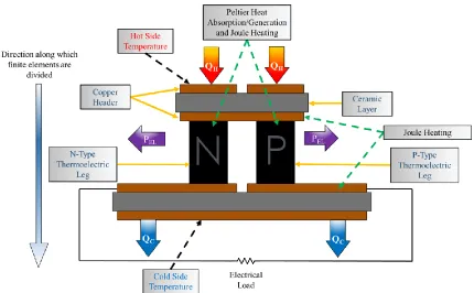
boundaries and joule heat generation in the unicouple. Joule heat generation occurs in the resistive elements of the electrical circuit, and net Peltier heat absorption occurs in the thermoelectric legs, as explained by Figure 7. The purpose of the ceramic layer is to act as an electrical insulator, while the copper headers connecting the legs aid in completing the electrical circuit and top and bottom copper headers are integrated with a heat exchanger or heat sink.

Figure 7: The unicouple components labelled. QH is the heat flow into the unicouple when the hot side temperature is maintained at a given value. Qc is the heat leaving the cold side of the unicouple when the cold side temperature is maintained at a fixed value. PEL is the thermoelectric power generated by the unicouple.

The heat transferred into a finite element containing a thermoelectric leg is given by the following equation:

𝑄ℎ,𝑝,𝑛 = 𝑎𝑏𝑠(𝛼𝑝,𝑛(𝑇)) ∙ (𝑇𝑛𝑜,𝑝,𝑛)∙ 𝐼 + 𝐾𝑝,𝑛(𝑇𝑛𝑜,𝑝,𝑛− 𝑇𝑛𝑜+2,𝑝,𝑛) − 1 2𝐼

2_{∙ 𝑅} 𝑒𝑙,𝑝,𝑛

(2-1) The heat leaving a finite element containing a thermoelectric leg is given by the following equation:

𝑄𝑐,𝑝,𝑛 = 𝑎𝑏𝑠(𝛼𝑝,𝑛(𝑇)) ∙ (𝑇𝑛𝑜+2,𝑝,𝑛)∙ 𝐼 + 𝐾𝑝,𝑛(𝑇𝑛𝑜,𝑝,𝑛− 𝑇𝑛𝑜+2,𝑝,𝑛) + 1 2𝐼

2_{∙ 𝑅} 𝑒𝑙,𝑝,𝑛

(2-2) where Qh,p,n is the heat transferred in to the p-leg and n-leg segments, and Qc,p,n is the heat transferred from the cold side of the p-leg and n-leg segments. The first terms on the right hand side of equations 2-1 and 2-2 account for the Peltier heat at the boundaries of the segment, where αp,n (T) is the temperature dependent Seebeck coefficient of each segment. Tno,p,n is the temperature of each element at the upper node of the element and Tno+2,p,n is the temperature of the bottommost node of each element, the nodes, and

elements of the model are shown in Figure 8(a). I is the current through the two legs, which are connected in series. The second term on the right side of equations 2-1 and 2-2 account for the thermal conduction through the thermoelectric legs, where Tno, p,n and Tno+2,p,n are defined as above. Kp,n is the thermal conductance of each element which is

given by the following equation:

𝐾𝑝,𝑛 =

𝜅𝑝,𝑛(𝑇)∙𝐴𝑝,𝑛 𝑙𝑝,𝑛

where κp,n (T)is the temperature dependent thermal conductivity in each segment, Ap,nis the area of each segment and lp,nis the height of each segment. The third term on the right hand side of equations 2-1 and 2-2 account for any Joule heat produced in the elements. The model assumes that half the Joule heat is transferred to the top of the element and the other half is transferred to the bottom of the element. Rel,p,n is the electrical resistance of each segment defined as follows:

𝑅𝑒𝑙,𝑝,𝑛 =

𝜌𝑝,𝑛(𝑇) ∙ 𝑙𝑝,𝑛

𝐴𝑝,𝑛

(2-4) where ρp,n (T) is the temperature dependent electrical resistivity of each segment. The

thermoelectric power generated in each segment is obtained by the difference between Qh,p,n and Qc,p,n in each segment described the following equation:

𝑃𝑝,𝑛= 𝑄ℎ,𝑝,𝑛− 𝑄𝑐,𝑝,𝑛 (2-5) The open circuit voltage is critical in obtaining the current through the circuit and is obtained by summing the individual voltage drops across each segment. The electric current through the unicouple is obtained using the open circuit voltage across the unicouple by the following equations:

𝑉𝑜𝑐 = ∑(𝛼𝑝(𝑇) − 𝛼𝑛(𝑇)) 𝑁

𝑖=1

(𝑇𝑛𝑜− 𝑇𝑛𝑜+2)

(2-6)

𝐼 = 𝑉𝑜𝑐 𝑅𝑒𝑙,𝑇𝐸𝐶+ 𝑅𝑒𝑙,𝐿

(2-7)

Figure 8: (a) The division of the unicouple along its vertical length into finite elements and the corresponding nodes, each element shares a node with its neighboring element (b) The simplified thermal circuit for the unicouple and the components of the unicouple

Temperature Profile

global stiffness matrix and a forcing vector. The temperature profile can be obtained by the matrix solution as follow:

𝑇 = 𝐾−1𝐹 (2-8)

where T is the temperature vector, K-1 is the inverse global stiffness matrix, and F is the forcing vector. The assembly of the global stiffness matrix requires elemental stiffness matrix, which is obtained as follows [21]:

𝐾𝑒= ∫ [𝐵]𝑇[𝐷][𝐵]𝐴𝑒𝑑𝑥 𝑘

𝑙

(2-9)

where B is a term borrowed from structural mechanics called the strain displacement matrix, the D matrix contains the elemental thermal conductivity terms, and Ae is the area of the element. The model uses one-dimensional quadratic elements, which allows an accurate solution to be obtained with a smaller number of elements in comparison to linear elements. The elemental stiffness matrix for this model simplifies to the following equation:

𝐾𝑒=

𝐴𝑒𝑘𝑒

𝑙𝑒

[

14 −16 2 −16 32 −16

2 −16 14

] _(2-10)

the elemental area. For a one-dimensional quadratic element, the forcing vector reduces to the following vector:

𝐹𝑒=

𝐺𝑒𝐴𝑒𝑙𝑒

6 [ 1 4 1

] (2-12)

where Ge is the elemental volumetric energy generation/absorption, Aeand leare defined as above. Once again, the global loading vector was assembled using each of the

elemental loading vectors while considering that each element has three temperature nodes.

It must be noted that an initial temperature profile (initial guess) is needed to obtain the required terms for the elemental stiffness matrix (temperature dependent thermal conductivity) and forcing vector (thermoelectric power generation in an

∑ 𝑎𝑏𝑠(𝑇𝑜𝑙𝑑(𝑖)− 𝑇𝑛𝑒𝑤(𝑖)) 𝑒𝑙𝑒𝑚𝑠

𝑖=1

< 𝐶𝐶

(2-13)

where Told is the temperature profile obtained from the previous iteration, Tnewis the new temperature profile, elems is the number of elements and CC is the convergence criteria set equal to 1°C. Once the final temperature profile is obtained, it is used in equations 2-1 through 2-7 to obtain the thermoelectric power generated by a unicouple.

Contact Resistance

The brazing process between the thermoelectric legs and headers can induce an electrical resistance. The electrical contact resistance is captured into the overall circuit, by adding it as an additional resistor, using an electrical resistivity of 1*10-9Ω-m2 [22]. The electrical contact resistivity was obtained from experimental data and numerical simulations. The electrical contact resistance is obtained using the following equation:

𝑅𝑐𝑜𝑛𝑡=

𝜌𝑐𝑜𝑛𝑡

𝐴𝑐

(2-14)

where ρcont is the electrical contact resistivity value of 1*10-9Ω-m2, and Acis the area of contact between the legs and the copper headers.

Model Validation

The one-dimensional model was compared with a 3-D model developed in an ANSYS environment for three different material types. The ANSYS model was

Table 1 Dimensions of the unicouple elements

Component Thickness/Height [mm] Area [mm x mm]

Copper Header 1 0.203 [1.93 * 1.96]*2

Ceramic 1 0.635 2.26 * 4.51

Copper Header 2 0.203 1.96 * 4.21

P-Leg 2.400 1.50 * 1.50

N-Leg 2.400 1.50 * 1.50

Copper Header 3 0.203 [1.96 * 4.07]*2

Ceramic 2 0.635 2.26 * 8.81

Figure 9: (a) Thermoelectric unicouple that was experimentally tested with results in Figure 11. (b) Temperature profile along unicouple for the 3-D ANSYS model for a hot side temperature of 600°C and cold side temperature of 100 °C, the results from the ANSYS model are available in Figure 11, Figure 14, and Figure 16

The ANSYS model developed was used to compare results from the finite element model for two additional materials, Bi2Te3 and PbTe with the temperature

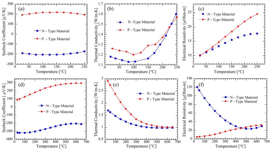
Figure 10: Temperature dependent properties of the Bi2Te3 material (a) Seebeck

Coefficient (b) Thermal Conductivity (c) Electrical Resistivity. Temperature dependent properties of the PbTe material (d) Seebeck Coefficient (e) Thermal Conductivity (f) Electrical Conductivity.

The results for the Half-Heusler alloy unicouple was compared for hot side temperatures of 200 °C, 300 °C, 400 °C, 500 °C and 600 °C while maintaining the cold side temperature at 100 °C as illustrated in Figure 11. The power results for the Half-Heusler material compare fairly well with the ANSYS model with an average percent error of 11.93%. The discrepancies in the power values are due to differing values of the leg hot and cold side temperatures. The temperature difference between the leg hot and cold sides influence the open circuit voltage of the unicouple, which in turn affects the power produced by the unicouple. The leg hot side temperature (T3 from Figure 8) is lower in the

3-D model compared to the 1-D model. Similarly, the leg cold side temperature (T4 from

3-D model as shown by the lateral temperature variations in Figure 12. The 1-3-D model assumes temperature variation along the vertical direction only, and lateral heat spreading is not accounted for. The average percent difference for the efficiency is 2.57%, the errors in the power calculations are carried over to the efficiency calculations, however, they are offset to a certain degree by the overestimation of the heat flowing into the unicouple.

Figure 11: (a) Peak thermoelectric power generation of a unicouple composed of the Half-Heusler alloy compared to a 3D ANSYS Model and experimental data. (b) Unicouple efficiency compared with a 3D ANSYS Model and experimental data.

The discrepancies of the finite element model with the experimental results are explained by an underestimation of the electrical contact resistivity included in the finite element model. Furthermore, the finite element model fails to account for any thermal contact resistances between contacting surfaces, which are experienced by the

Figure 12: A cross-sectional view of the bottom surface of the n-type leg. Lateral temperature variations are observed in the ANSYS model, which is not accounted for in the 1-D finite element model.

The power and efficiency curves obtained by varying the load resistance are displayed in Figure 13 (a) and (b) for the five different hot side temperatures. The device voltage decreases from the open circuit voltage to zero as the current is increased by varying the load resistance as shown in Figure 13(c). The maximum power is obtained at a device voltage that is equal to half the open circuit voltage.

Similarly, the power generated and efficiency was compared for a unicouple composed of Bi2Te3. The hot side temperature was increased from 50°C, 100°C, 150 °C,

200°C and 250°C, which is its operating limit while maintaining the cold side temperature at 20 °C. The power and efficiency results are compared in Figure 14. The average percent error in the power calculations is 2.73% for the Bi2Te3 material, whereas the average

percent error for the efficiency calculation is 14.2%. The better accuracy in the power calculations are accounted for by smaller discrepancies in the leg hot (T3 from Figure 8)

and cold side temperatures( T4 from Figure 8) when compared with the 3-D ANSYS model.

The discrepancies in the heat flow are attributed to the model underestimating the heat flow into the model, considering 3-D heat spreading effects are not accounted for in the model.

Figure 14: (a) Peak thermoelectric power generation of a unicouple made of the Bi2Te3 material compared to a 3D ANSYS Model (b) Unicouple efficiency compared

with a 3D ANSYS Model.

The power and efficiency curves obtained by varying the load resistance is displayed in Figure 15. The electrical current values are restricted by the open circuit voltage values, which are smaller for the unicouple composed of the Bi2Te3 material

Figure 15: (a) Thermoelectric Power Generated for varying current for a unicouple composed of the Bi2Te3 material (b) The TEG efficiency for varying current

for a unicouple composed of the Bi2Te3 material (c) Device voltage vs. electric current

for a unicouple composed of the Bi2Te3 material.

Figure 16: (a) Peak thermoelectric power generation of a unicouple composed of the PbTe material compared to a 3D Ansys Model (b) Unicouple efficiency compared with a 3D Ansys Model

Similar to the Half-Heusler alloy unicouple and Bi2Te3 unicouple, the power and

efficiency curves were obtained by varying the load resistance, which resulted in the power and efficiency curves in Figure 17 (a) and (b). The accompanying voltage vs. current curves are displayed in Figure 17(c).

Figure 18: (a) Power density vs. temperature difference compared with experimental results. (b) Open circuit voltage vs. temperature difference compared with experimental results [23].

Ceramic Material

The thermoelectric power generated by a unicouple can be increased by having the largest possible temperature difference between the thermoelectric legs (temperatures T3

and T4 from Figure 8). For the Half-Heusler material model described in the previous

ceramic currently used Alumina (Al2O3) varies from 24.7 W/m-K at room temperature to

6.59 W/m-K at 600°C as illustrated in Figure 19. Three other electrical insulators with better thermal conductivities are considered in this section. The three materials of interest are Aluminum Nitride, Silicon nitride, and Beryllium oxide. Alumina is the industry standard for electronic substrates [24] and is the ceramic chosen in the model in the previous section. It offers the advantages of having relatively high strength, a high service temperature, being chemically inert and having a lower cost when compared to the other materials. Beryllia (BeO) has the highest thermal conductivity values of 259.4 W/m-K at room temperature and 46.79 W/m-K at 600°C among the materials considered. However, it is extremely expensive due to high powder costs. Furthermore, it is also considered a toxic substance, which limits its application. Aluminum nitride (AlN) has a thermal conductivity of 200 W/m-K at room temperature and 40.46 W/m-K at 600°C, which is comparable to the thermal conductivity of Beryllia. It offers a non-toxic alternative to Beryllia and has good oxidation resistance, which is significant at high temperatures. However, similar to Beryllia it is expensive and is only feasible in limited applications. Silicon nitride (Si3N4) has thermal conductivity values of 63.5 W/m-K at room temperature

shock resistance, which makes it an attractive material for high-temperature applications [25].

Figure 19: Thermal Conductivity vs. Temperature comparison of ceramics that can be used as an electrical insulator for a unicouple [25]

Figure 20: Temperature profile of the unicouple for a unicouple that has Alumina as the ceramic and Beryllia as the ceramic; the green lines are used to indicate the temperature along the thermoelectric legs.

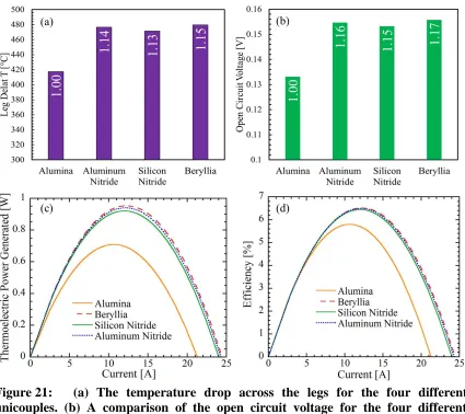
The improvements in the open circuit voltages are 1.16 for Aluminum Nitride, 1.15 for Silicon Nitride and 1.17 for Beryllia when compared with the open circuit voltage of the unicouple with Alumina as the ceramic. The enhancements in the power results are 1.33 for Aluminum Nitride, 1.30 for Silicon Nitride and 1.34 for Beryllia when compared with the power output of the unicouple with Alumina as the ceramic as shown in Figure 21(c). It is interesting to note that although the Beryllia material has a higher overall thermal conductivity compared to Aluminum Nitride and Silicon Nitride, the improvements in the thermoelectric power are comparable to the unicouples with AlN and Si3N4 as the

Figure 21: (a) The temperature drop across the legs for the four different unicouples. (b) A comparison of the open circuit voltage for the four different unicouples (c) Power generated vs. electric current comparison for unicouples composed of the four different ceramic material (d) Efficiency vs. electric current for unicouples made of the different ceramic

The enhancements in the power results are approximately a square of the improvements in the open circuit voltage, which are validated by the fact that the thermoelectric power for the maximum power condition from a unicouple can be approximated by the following equation:

𝑃𝑇𝐸𝐶 =

𝑉𝑜𝑐2

4 ∙ 𝑅𝐿

(2-15)

unicouple with a ceramic composed of Aluminum Nitride, 1.11 for one with Silicon Nitride, and 1.12 for one with Beryllia, which corresponds to the increase in the temperature difference across the legs.

Segmented Leg Unicouples

One of the major limitations of thermoelectric generators holding it back from large-scale production is their low heat-to-power conversion efficiencies. The conversion efficiency is itself capped by the Carnot efficiency η = (Th –Tc)/Th as demonstrated by

equations 1-6 and 1-7. The conversion efficiency is dependent upon the thermoelectric figure of merit, which is temperature dependent as illustrated in Figure 22, suggesting that certain thermoelectric materials perform better at specific temperatures.

Figure 22: (a) ZT of the N-Type for the respective materials. (b) ZT of the P-Type for the respective materials (c) Compatibility factor for the Half-Heusler alloy, PbTe material, and Bi2Te3 material.

Figure 23: A segmented TEG and cascaded TEG are illustrated using a single unicouple. The primary difference is the use of two different electrical loads connected to the different stages in the cascaded TEG and the use of a single circuit in the segmented TEG.

Thermoelectric Compatibility

materials as they would have different electrical resistivites. Furthermore, each material has its own optimum relative current density defined by the following equation [26]:

𝑢 = 𝐽 𝜅𝛻𝑇

(2-16)

where J is the electric current density, κ is the thermal conductivity and 𝛻T is the temperature gradient. If the relative current density of the two-segmented materials differs significantly, the thermoelectric efficiency may decrease when compared to using a single material [26]. The thermoelectric compatibility equation may be utilized to select materials, which can be used for segmentation:

𝑠 = √1 + 𝑧𝑇 − 1 𝛼𝑇

(2-17)

where ZT is the thermoelectric figure of merit, α is the Seebeck coefficient, and T is the absolute temperature. Initially, it was suggested that two materials with compatibility factors differing by a factor of 2 would decrease efficiency when segmented [27, 28]. However, Ouyang and Li suggest that it is the smooth transition of the compatibility factors at the temperature boundaries that is significant [29]. A smooth transition is observed in the compatibility factor for the p-type at 200°C for Bi2Te3 and PbTe, and a

similar transition can be witnessed for Bi2Te3 and Half-Heusler at 250 °C in Figure 22(c).

For the n-type material, the transition is observed at the limit of the Bi2Te3 operating

temperature of 250 °C. Additionally, it is also observed that the thermoelectric figure of merit of Bi2Te3 is larger than that of the Half-Heusler and PbTe materials from 20°C to

approximately 225 °C for the n-type material and 200°C for the p-type material. Design of Segmented Leg Unicouples

and the Half-Heusler material and the thermoelectric figure of merit of both materials, 250°C appears to be a suitable interface temperature. This observation means that the segmented unicouple would be designed such that the Bi2Te3 segment of the unicouple

will experience a temperature from 250 °C to 20 °C. Similarly, the Half-Heusler alloy segment will have a hot side temperature of 600°C, and a cold side temperature of 250°C. The total height of the unicouple was kept similar to that in Table 1. In order to obtain the required interface temperature, the thermal resistances of the segments have to be

adjusted according to the required interface temperature. While keeping the leg areas constant, the following equation can be utilized to obtain the ratio of the two segment heights [30]:

𝑙𝑝1

𝑙𝑝2

= ∫ 𝜆𝑝,1(𝑇)𝑑𝑇

𝑇ℎ 𝑇_𝑖𝑛𝑡

∫ 𝜆𝑝,2(𝑇)𝑑𝑇 𝑇𝑖𝑛𝑡

𝑇𝑐

(2-18)

𝑙𝑛1

𝑙𝑛2

= ∫ 𝜆𝑛,1(𝑇)𝑑𝑇

𝑇_ℎ 𝑇_𝑖𝑛𝑡

∫ 𝜆𝑛,2(𝑇)𝑑𝑇 𝑇𝑖𝑛𝑡

𝑇_𝑐

(2-19)

𝑙 = 𝑙𝑝1+ 𝑙𝑝2= 𝑙𝑛1+ 𝑙𝑛2 (2-20)

at the interface between the bottom copper segment and the bottom segment, and l is the total height of the combined leg. The leg heights of each segment obtained by equations 2-18 through 2-20 and are shown in Table 2.

Table 2 Height of the material segments in unicouple A and B

Segment Unicouple A Unicouple B

Half-Heusler alloy segment 2.106 mm

-PbTe segment - 1.618 mm

Bi₂Te₃ segment 0.294 mm 0.782 mm

Total Height 2.4 mm 2.4 mm

The power and efficiency curves are compared in Figure 24 for both the Half-Heusler-Bi2Te3 segmented unicouple (unicouple A) and the PbTe-Bi2Te3 segmented

unicouple (unicouple B) compared with only using a single material. The models were run for a hot side temperature of 600°C and cold side temperature of 20°C and compared using similar geometric properties with the difference being leg heights defined in Table 2. For the segmented Half-Heusler unicouple there was a 16 % increase in the power output, while there was 61 % increase in the peak efficiency. The higher increase in the efficiency is explained by the fact that the compatibility factor is utilized to find matching materials, which can be used to improve efficiency. While improvements in power

generation are expected with improved efficiency, the primary improvement is in the heat to power conversion efficiency. Similarly, for the PbTe-Bi2Te3, segmented unicouple a

Figure 24: (a) Thermoelectric power and (b) efficiency comparison for the Half-Heusler-Bi2Te3 unicouple compared to a unicouple composed only of the Half-Heusler

alloy. (c) Thermoelectric power and (d) efficiency comparison for the PbTe-Bi2Te3

THERMOELECTRIC GENERATOR – HEAT EXCHANGER MODEL

Introduction

Thermoelectric generators are often accompanied by heat exchangers with the goal of maintaining the required temperature difference across a thermoelectric module. Compact heat exchangers are used in waste heat recovery when there is a restriction on the available space, for instance in automotive waste heat recovery applications [3]. Further, applications of compact heat exchangers include high-temperature polymer electrolyte membrane fuel cell exhaust heat recovery [19] and waste heat reclamation from jet engines[5]. Heat exchangers, which utilize forced convection, are often used, as the waste heat is often available as a flowing hot fluid.

temperature dependent fluid and thermoelectric properties.

Model Assumptions

The following assumptions were made to simplify the heat exchanger model. 1) The model divides each spacing in the heat exchanger as an individual channel,

which leads to the following assumptions

a. The mass flowrate in each channel is identical and is obtained by dividing the total flowrate by the number of channels.

b. The heat transfer coefficient and friction factor in each section of the channel is constant for the control volume.

2) Lateral variations in temperature are ignored.

3) The model assumes the flow is fully developed when entering each channel. The heat exchangers are usually accompanied by a diffuser, which is not included in the model.

4) Constant fluid temperatures are assumed in each control volume and a constant fin base temperature is assumed for each control volume.

Control Volume – Energy Balance

The model is solved by portioning each segment of the TEG-heat exchanger system into finite control volumes as illustrated in Figure 22. The fundamental principal used to solve the model is the first law of thermodynamics, by equating the heat flow through the fins to be equal to the heat flow through the thermoelectric modules. The TEG-Heat exchanger model is split into two symmetric components as shown in Figure 25 and calculations are performed on one section to minimize computational expense. The length of one control volume needs to be the length of the thermoelectric module.

Figure 25: TEG – Heat Exchanger model illustrated with a 3-D view, front view and a side view explaining the energy balance concept used in the model. QH is the heat flow into the hot side of the TEG within the control volume and QC is the heat flow from the cold side of the TEG to the cold-side heat exchanger. QFH is the heat flow from the hot side heat exchanger within the control volume and QFC is the heat flow from the cold-side heat exchanger in the control volume. PEL is the thermoelectric power generated by the TEG.

The heat flow through the heat exchanger in the control volume is given by the following equation by using the adiabatic fin tip condition [31]:

𝑄𝑓 = 𝑀 ∙ 𝑡𝑎𝑛ℎ (𝑚 ∙

𝑓ℎ

2) ∙ (𝑁𝑓− 1) + 𝐴𝑢𝑓∙ ℎ ∙ (𝑇𝑏− 𝑇𝑓)

base temperature of the control volume, Tfis the fluid temperature within the control volume and h is the channel convection coefficient which will be discussed in detail in the next section. P is the fin perimeter, k is the thermal conductivity of the fin material, and Ac is the cross-sectional area of the fin. The heat flow into the module, Qh is equal to the heat transferred through the fins in the control volume, while the heat flow leaving the cold side of the module, Qc is equal to the heat transferred through the cold side heat exchanger, QFC. The difference between the heat entering and leaving the module is equal to the thermoelectric power generated by the module as explained in the previous chapter. An iterative process solves the TEG-Heat Exchanger model, and the energy balance criteria have to be met for each control volume. The difference between the heat flow through the hot side of the heat exchanger (QFH) and the heat flow into the module (QH) has to be less than the required convergence criteria of 10-4W. Similarly, the

𝑇𝑓,𝑜𝑢𝑡 = 𝑇𝑓,𝑖𝑛−

𝑄𝑓

𝑚̇ ∙ 𝑐𝑝

(3-4)

where Tf,outis the exit temperature of the fluid in the control volume, Qf is the heat transferred by the heat exchanger within the control volume, 𝑚̇ is the mass flowrate and cp is the specific heat of the fluid.

Channel Convection Coefficient

The channel convection coefficient utilized in the model are obtained from available empirical correlations. Similar numerical models [16, 17] have used Reynolds number dependent empirical correlations for the convection coefficients for channel flow. The current model uses convection coefficients for smooth rectangular ducts, which are dependent upon the channel width to height ratio. The hydraulic diameter, dh dependent

Reynolds number for the channel flow is obtained by the following equations:

𝑅𝑒 =𝑣𝑐ℎ∙ 𝑑ℎ 𝜈𝑓

(3-5)

𝑑ℎ=

4 ∙ 𝐴

𝑃 (3-6)

where vch is the channel velocity, νf is the kinematic viscosity, P is the wetted perimeter, and A is the channel cross-sectional area. The critical Reynolds number for a rectangular inlet geometry varies from 2000 to 3100 with the upper limit at 10000 [32]. For this model, laminar and turbulent flow is analyzed with the critical Reynolds number being 2500 based on the empirical correlation used. The convection coefficient evaluated using the Nusselt number relationships for the laminar and turbulent regions are obtained using the following equations [32]:

𝑁𝑢 = 7.541 ∙ (1 − 2.61𝛼 + 4.970𝛼2− 5.199𝛼3+ 2.702𝛼4− 0.548𝛼5) 𝑅𝑒 ≤ 2500

number, Pr is the Prandtl number, kf is the fluid thermal conductivity,dh is the hydraulic diameter defined above, Tsis the surface temperature, and Tfis the fluid temperature.

Compact heat exchangers defined as having a surface area of 650 m2 per cubic meter [33] are widely used in applications such as automotive waste heat recovery due to spatial constraints. The following equations developed by Weiting [34] for compact rectangular offset plate fin heat exchangers are considered in the model as well:

𝑗 = 0.483 ∙ (ℎ𝑥𝑙

𝑑_ℎ)

−0.162_{∙ 𝛼}−0.184_{∙ 𝑅𝑒}−0.536 _{Re ≤ 1000 (3-11)}

𝑗 = 0.242 ∙ (ℎ𝑥𝑙

𝑑ℎ)

−0.322_{∙ (}𝑡𝑓 𝑑ℎ)

−0.089_{∙ 𝑅𝑒}−0.368 _{Re > 1000 (3-12)}

ℎ = 𝑗 ∙ 𝑅𝑒 ∙ 𝑃𝑟1/3∙𝑘𝑓 𝑑ℎ

thickness is not included in the correlation for the laminar region, suggesting the influence of the fin thickness is limited in laminar flow [34].

Model Validation

The TEG heat exchanger model was compared with an available computational fluid dynamics and ANSYS model, which was developed for a TEG-Heat Exchanger system for automotive waste heat recovery from a diesel engine [3]. The model was compared using the convection coefficients for duct flow using equations 3-10 and the convection coefficients for compact offset fin heat exchangers using equation 3-13. The model was compared for fin packing fractions of 10%, 15%, 20%, 25%, and 30 % and fin thicknesses of 0.1mm, 0.2mm, 0.3mm and 0.4 mm encompassing in 20 different designs. The exhaust of a car resemble the properties of air, and the temperature dependent

Figure 26: Input parameters for the TEG – Heat exchanger model. Four modules with a fixed cold side temperature are combined with the hot side heat exchanger.

Table 3 Input to the TEG – Heat Exchanger Model

Input Value

Exhaust Inlet Temperature 558 °C

Hot Side Fluid Exhaust gas (Air)

Number of Modules 4

Module Size 40mm x 40 mm x 4.9 mm

TEM Cold Side Temperature 94 °C

Heat Exchanger Width 40 mm

Heat Exchanger Length 160 mm

Heat Exchanger Height 20 mm

Heat Exchanger Material Nickel

channels and a larger fin surface area, resulting in better heat flow compared to the other heat exchanger designs. However, the better thermal performance comes at the cost of a larger pressure drop across the heat exchanger. The model using the compact heat

exchanger convection coefficient appears to show more consistent results when compared with the model using the duct convection coefficient. The discrepancies between the two models developed can be attributed to the limitations of the empirical convection

coefficients used and the lateral heat spreading that is captured in the 3-D model. The mismatch in convection coefficients between the models results in a mismatch in the heat transferred through the heat exchanger, which can be used to explain the discrepancies observed in Figure 27. Furthermore, the model accuracy could be improved by

Figure 27: The average heat flow through each module compared with a 3D Model using the TEG – Heat Exchanger Model that uses compact heat exchanger convection coefficients and duct convection coefficients for (a) fin thickness = 0.1 mm (b) fin thickness = 0.2 mm (c) fin thickness = 0.3 mm (d) fin thickness = 0.4 mm[3].

The average percent difference between the models using the two different types of convection coefficients are compared in Table 4. The compact heat exchanger

Table 4 Average percent error comparison between the two models. The percent error values are obtained assuming the 3-D model values as the exact or theoretical value.

Fin Thickness Duct Convection Coefficient model

Compact Heat-Exchanger Convection Coefficient

model

0.1 mm 7.60 % 7.50 %

0.2 mm 5.79 % 4.63 %

0.3 mm 6.37 % 4.36 %

0.4 mm 8.13 % 4.76 %

Figure 28: The average temperature difference across each module compared with a 3D Model using the TEG – Heat Exchanger Model that uses compact heat exchanger convection coefficients and duct convection coefficients for (a) fin thickness = 0.1 mm (b) fin thickness = 0.2 mm (c) fin thickness = 0.3 mm (d) fin thickness = 0.4 mm[3].

drop compared to the other designs. When the heat exchanger design is considered both pressure drop and heat transfer capabilities of the heat exchanger should be evaluated.

Introduction

Natural convection heat sinks can be incorporated with TEGs to maintain the cold side temperature of the TEG. There are many instances when it is not possible to

integrate a forced convection heat sink with a TEG, for instance when a TEG is used to recover waste heat from the body. Furthermore, natural convection heat sinks are much more reliable than forced convection heat exchangers. Natural convection heat sinks require almost no maintenance, which makes them ideal to be implemented with TEG devices that are used to self-power electric devices. Additionally, natural convection heat sinks require no pumping power, as compared to forced convection heat sinks, which means that all the power generated by a TEG can be used to power devices, and none of the energy is expended on pumping power. However, heat transfer coefficients for natural convection heat sinks are much smaller than forced convection heat exchangers.

different types of heat sinks are illustrated in Figure 30 with their orientation with respect to the gravitational field shown. The heat sinks are then optimized to be used with a TEG to power a wireless sensor using waste heat from a pipe in a nuclear power plant. Finally, optimized heat sinks are combined with TEGs to harvest waste body heat which can be used to power wearable electronics.

Figure 30: The three different types of heat sinks considered in this section.

Vertical Flat Plate Heat Sink Model

As stated in the introduction section, the primary difference between the heat sink models are the convection coefficients of the heat sinks. Natural convection coefficients for parallel plate heat sinks are obtained from work done by Bar-Cohen et al. [35]. The convection coefficient builds on work initially done by Bar-Cohen [36]. It is important to note the convection coefficient apply to finned geometries, which takes into consideration asymmetric heat flow. A 1-D analytical steady state model is developed to predict the thermal performance of vertically oriented natural convection plate fin heat sinks. The primary direction of heat transfer is from the base of the heat sink to the ambient.

𝑄𝐻𝑆= 𝑛𝑓𝑖𝑛∙ 𝑞𝑓𝑖𝑛+ ℎ𝑏𝑎𝑠𝑒∙ 𝐴𝑏∙ (𝑇𝑏− 𝑇𝑎𝑚𝑏) (4-2)

where nfinis the number of fins, Abis the unfinned base area, Tbis the heat sink base temperature, and hbase and qfinare defined by the following equations. The unfinned base area is treated as a vertical flat plate, and the convection heat transfer coefficient is obtained as follows:

ℎ𝑏𝑎𝑠𝑒 = 0.59 ∙ 𝑅𝑎𝐿 1/4

∙ 𝑘𝑓⁄𝐿 (4-3)

where kf is the thermal conductivity of air, and L is the vertical length of the heat sink, and the Rayleigh number, RaLis obtained as follows:

𝑅𝑎𝐿= 𝑔 ∙ 𝛽 ∙ 𝜃𝑏∙ 𝑃𝑟 ∙ 𝐿3⁄𝜈2 (4-4) where g is gravity, β is the coefficient of thermal expansion, θb is the temperature

difference between the heat sink base and the ambient, Pr is the Prandtl number, and ν is the kinematic viscosity of the fluid. The heat transfer from each of the individual plate-fins, qfin, is obtained as follows[31]:

𝑞𝑓𝑖𝑛 = 𝑀 ∙ 𝑡𝑎𝑛ℎ (𝑚 ∙ 𝐻) (4-5) where H is the height of the plate fins extruding in the horizontal direction, M and m are fin parameters defined as follows:

𝑚 = √(ℎ ∙ 𝑃) (𝑘 ∙ 𝐴⁄ 𝑐) (4-7) where k is the thermal conductivity of the fin material, P is the fin perimeter, and Ac is the cross-sectional area. The convection heat transfer coefficient, h from non-isothermal asymmetric plates, take into account the two limiting spacing conditions for flat plate heat sinks, small fin spacing, and large fin spacing. The convection coefficient considering the spacing limits above is obtained as follows [35]:

ℎ𝑓𝑖𝑛 =

𝑘𝑎

𝑠 ∙ (

576 (𝜂𝑓𝑖𝑛∙ 𝐸𝑙)2

+ 2.873 (𝜂𝑓𝑖𝑛∙ 𝐸𝑙)

1 2

)1/2 (4-8)

where s is the spacing between the plate fins, ηfin is the fin efficiency, and El, the Elenbaas number, which is a modified version of the Rayleigh number, is obtained as follows:

𝐸𝑙 = (𝑔 ∙ 𝛽 ∙ 𝜃𝑏∙ 𝑃𝑟 ∙ 𝑠4) 𝐿𝜐⁄ 2 (4-9)

The first term in parentheses in equation 4-8 accounts for the small fin spacing condition, while the second term represents the large spacing condition. When the heat sink is used for applications with large temperature differences, radiation effects become significant and are considered in the heat sink model. Radiation heat transfer from the outer surfaces of the heat sink was considered in the model, as these surfaces have a view factor of 1 with the ambient. The heat transfer by radiation is given by the following equation:

Vertical base pin fin heat sinks are another viable option to be used along with TEGs to harvest waste thermal energy. Pin fin heat sinks have better thermal performance compared to flat plate heat sinks when the mass of the heat sink is considered [37]. A one-dimensional heat transfer model is developed similar to the vertical flat plate heat sink model. The primary differences between the two models are the fin geometry, the fin cross-sectional area, and the fin perimeter. In addition to the fin geometry, the convection coefficient for pin fin heat sinks is different to that of the vertical plate heat sinks. The convection coefficient for pin fin heat sinks are influenced by four limiting conditions, which are listed below:

1) Small vertical spacing with small horizontal spacing 2) Small vertical spacing with large horizontal spacing. 3) Large vertical spacing with small horizontal spacing. 4) Large vertical spacing with large horizontal spacing.

The work done by Joo et al. [37] consider convection coefficients for each limiting case and combine them to match empirical data. The convection coefficient for limiting case 1 looks at densely packed heat sink with a large number of pins in both the

ℎ𝑓𝑖𝑛,1=

𝑆ℎ𝑆𝑣

𝜋𝑑𝐿 ∙

4𝑆ℎ𝑆𝑣− 𝜋𝑑2

48 ∙

𝜌𝑓𝑐𝑝𝑔𝛽𝜂𝑓𝑖𝑛(𝑇𝑏− 𝑇∞)

𝜐𝑓

(4-11)

where Sh and Sv are the horizontal and vertical spacing, d is the fin diameter, L is the heat sink length, ρf is the fluid density, cpis the specific heat of the fluid, g is the acceleration of gravity, β is the thermal coefficient of expansion, ηfinis the fin efficiency, νf is the kinematic viscosity of the fluid, Tbis the base temperature and T∞ is the ambient temperature. For the second limiting case, the pins are arranged in a vertical direction with large horizontal spacing and can be modelled as an isolated vertical array of cylinders by the following equation:

ℎ𝑓𝑖𝑛,2=

𝑘𝑓

𝐿 ∙ [0.3669

𝑆_𝑣

𝑑 − 0.0494] 𝐺𝑟𝐿

1/4 (4-12)

𝐺𝑟𝐿=

𝑔𝛽𝜂𝑓𝑖𝑛(𝑇𝑏− 𝑇∞)𝐿3

𝜐_𝑓2

(4-13)

where GrL is the length dependent Grashof number and the other variables as defined above. For the third limiting case, pins are arranged in a single horizontal direction with large vertical spacing, and the convection coefficient is obtained by the following equation:

ℎ𝑓𝑖𝑛,3=

𝑘𝑓

𝑑 ∙ [2.132𝑆ℎ

∗_{− 0,4064](}𝑔𝛽(𝑇𝑏− 𝑇∞)

𝛼𝑓𝜐𝑓𝑑

)0.188 (4-14)

𝑆ℎ∗=

𝑆_ℎ∗ 𝑑3/4_𝐿1/4

(4-15)