https://doi.org/10.5194/wes-4-369-2019
© Author(s) 2019. This work is distributed under the Creative Commons Attribution 4.0 License.
A vortex-based tip/smearing correction
for the actuator line
Alexander R. Meyer Forsting, Georg Raimund Pirrung, and Néstor Ramos-García
DTU Wind Energy, Technical University of Denmark, Frederiksborgvej 399, 4000 Roskilde, Denmark
Correspondence:Alexander R. Meyer Forsting ([email protected])
Received: 21 December 2018 – Discussion started: 21 January 2019 Revised: 13 May 2019 – Accepted: 16 May 2019 – Published: 28 June 2019
Abstract. The actuator line (AL) was intended as a lifting line (LL) technique for computational fluid dynamics (CFD) applications. In this paper we prove – theoretically and practically – that smearing the forces of the actuator line in the flow domain forms a viscous core in the bound and shed vorticity of the line. By combining a near-wake representation of the trailed vorticity with a viscous vortex core model, the missing induction from the smeared velocity is recovered. This novel dynamic smearing correction is verified for basic wing test cases and rotor simulations of a multimegawatt turbine. The latter cover the entire operational wind speed range as well as yaw, strong turbulence and pitch step cases. The correction is validated with lifting line simulations with and without viscous core, which are representative of an actuator line without and with smearing correction, respectively. The dynamic smearing correction makes the actuator line effectively act as a lifting line, as it was originally intended.
1 Introduction
The actuator line (AL) technique developed by Sørensen and Shen (2002) is a lifting line (LL) representation of the wind turbine rotor suitable for computational fluid dynam-ics (CFD) simulations. It captures transient physical features like shed and trailed vorticity (including root/tip vortices), without the computational cost associated with resolving the full rotor geometry. Thus, the AL model enables large-eddy simulations (LES) of large wind farms in realistic, turbulent atmospheric boundary layers (Vollmer et al., 2017).
However, in contrast to LL vortex formulations, the blade forces are dispersed in the flow domain – most commonly in form of a Gaussian projection – to avoid numerical instabili-ties. A length scale – also referred to as smearing coefficient – controls this force redistribution, the lower limit of which is linked to the grid size by numerical stability requirements (Troldborg et al., 2009). Mikkelsen (2003) observed a large sensitivity of the blade velocities to this length scale, which consequently also propagated to the blade forces. Especially in regions along the blade exhibiting stark load changes, such as around the root and tip, forces are substantially over-predicted, meaning that this effect is exacerbated by
non-tapered and low-aspect-ratio blades. As actuator disc for-mulations suffer from similar issues towards the blade tip, Glauert (1935) type tip corrections are also frequently ap-plied to ALs (Shen et al., 2005). However, these correct discs for missing discrete blades and should therefore be unneces-sary – strictly even invalid – for ALs. Shives and Crawford (2013) and Jha et al. (2014) achieved a reduction in the force over-prediction by varying the originally fixed smearing fac-tor with respect to the blade chord. However, their methods cannot decouple the blade forces from the smearing length scale: a smeared force distribution in the flow domain un-avoidably leads to lower induction at the blade – increasing lift and drag – compared with an actual LL with a concen-trated, spatially singular force.
1.1 The vortex smearing hypothesis
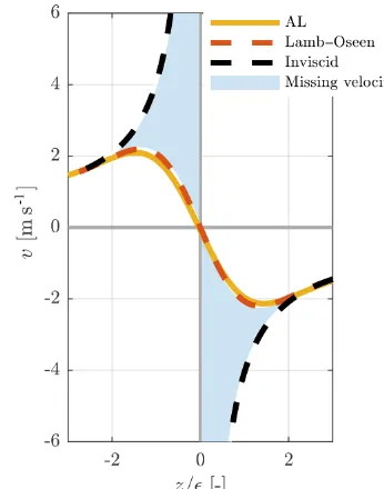
Fig. 1 – here with a Lamb–Oseen vortex core model (Lamb, 1932; Oseen, 1911). Without viscosity (inviscid) the veloci-ties approach infinity towards the vortex centre. The startling agreement between the Lamb–Oseen and AL velocities was first demonstrated by Dag et al. (2017). The Gaussian body force smearing in the AL technique thus produces similar swirl velocities to a viscous vortex. Ignoring viscous effects, the AL should, in principle, induce the same velocities as a LL – equivalent to the inviscid solution. The missing induced velocity in the AL model (shaded area in Fig. 1) can be ap-proximated following Dag et al. (2017) as follows:
1vθ(r)=
inviscid
z }| { 0
2π r −
viscous core
z }| {
0
2π r h
1−exp−r2/2i
= 0 2π rexp
−r2/2, (1)
where0represents the vortex line’s circulation,ris the dis-tance from the vortex core andis the length scale used in the force smearing. This formulation can be split into an in-viscid and viscous/smearing contribution:
1vθ(r)=
inviscid
z }| { vθ(r)f(r)
| {z }
smearing
with vθ(r)= 0
2π r,
f(r)=exp(−r2), r=r
. (2)
If this viscous behaviour of the force smearing in AL simula-tions was limited to the bound vortex representing the blade, it would not influence the blade forces as long as the blade was straight. However, Dag et al. (2017) argued that the trail-ing vortices (in the wake) exhibit the same viscous core, as they originate from the bound vortex. Hence, the wake of an AL induces lower velocities at the blade than a LL. The miss-ing velocity can be estimated from the viscous core equiva-lence and thus correct the velocities at the blade. This mostly impacts blade forces by changing the angle of attack at the blade sections.
1.2 Contributions of this paper
Dag et al. (2017) corrected AL simulations of a rectangular wing and two rotors with different aspect ratios by recuper-ating the missing induced velocity introduced by the viscous core. For all of their simulations they were able to show the beneficial effect of the correction on the blade load distribu-tion – represented by more physical behaviour, especially to-wards the tip and root. However, their implementation of the correction did not fully couple the flow field with the blade forces and the induction correction.
The major contributions of this paper are as follows:
– The development of a tuning-free, dynamic and numeri-cally robust smearing correction, which is fully coupled to the AL model.
Figure 1.Distribution of the tangential velocity component in a plane orthogonal to an infinite vortex line (alongx) obtained from either an inviscid or viscous (Lamb–Oseen) theoretical vortex and an actuator line (AL) CFD simulation.
– A theoretical proof of the force smearing – vortex core equivalence.
– Proof of the vortex core inheritance in trailed vorticity.
– The confirmation of the missing velocity assumption by comparing LL simulations with/without viscous core and AL results with/without correction.
The test cases include constantly and elliptically loaded wings as well as rotor simulations of a multimegawatt tur-bine covering the entire operational wind speed range. As the AL model is especially attractive for wind farm simula-tions, the focus here is on coarsely resolved ALs. The correct dynamic behaviour of the new correction is verified through yawed inflow and pitch step simulations.
2 Proof of force smearing – vortex core equivalence
The equivalence between the velocity field induced by an AL and a viscous vortex can be derived directly from the incompressible Navier–Stokes equations. This proof follows the approach by Forsythe et al. (2015) that successfully con-nected an AL’s vorticity field to its force projection. Starting by taking the curl of the incompressible momentum equation, the vorticity transport equation is obtained (ω= ∇ ×u):
∂ω
∂t |{z}
=0 steady
+(u∇)ω=(ω∇)u
| {z } =0 2D
+ν∇2ω
| {z } =0 inviscid
+ ∇f
whereν is the viscosity,ρ is density and f represents the body forces from the AL. Away from the root and tip, the flow around a high-aspect-ratio blade is nearly two-dimensional, as the span-wise flow is negligible. Viscous effects are disregarded in light of the large Reynolds num-bers encountered. Furthermore the relationship between the body force and flow field becomes quasi-steady assuming the flow is attached. Cancelling the respective terms and not-ing that in two-dimensional flow (y−zplane)ω=ωxeˆxand
∇ =(0,∂y∂ ,∂z∂):
(u∇)ωxeˆx= ∇
f
ρ. (4)
Assuming the drag to be negligible, the force – in the form of lift – exerted by the AL on the flow in terms of its circulation
0becomes
f = −faerog(r) (5)
faero=L=ρu×0eˆx g(r)=
1
π 2exp(−r
2/2). (6)
Heregrepresents a two-dimensional Gaussian force projec-tion with r indicating the distance from the AL. Inserting these expression into Eq. (4) and exploiting standard matrix transformation and mass conservation1
(u∇)ωxeˆx= ∇(0geˆx×u)=(u∇)0geˆx (7)
(u∇)ωx=(u∇)0g. (8)
Due to mass conservation theu∇ term can be inverted; this gives a direct relationship between the force projection and vorticity:
ωx=0g= 0
π 2exp(−r
2/2). (9)
As the body force is axially symmetric, the vorticity only induces tangential velocities
ωx(r)=
1 r ∂ruθ ∂r − ∂ur ∂θ |{z} =0 axisymmetry
⇒uθ=
1
r r Z
0
rωx(r)dr. (10)
Inserting Eq. (9) and integrating gives the swirl velocity in-duced by a smeared body force
uθ= 0
2π r h
1−exp(−r2/2)i. (11)
1∇ ×(eˆ
x×u)=(u∇)eˆx−(eˆx∇)u+ ˆex(∇u)−u(∇ ˆex)=
(u∇)eˆx+0+0+0
This expression equals that of the Lamb–Oseen vortex, only with the viscous core radius replaced by the smearing coef-ficient2. This marks the theoretical confirmation of the ob-servations by Dag et al. (2017), which additionally indicates that a viscous core behaviour with an AL requires inviscid, two-dimensional and locally steady flow conditions.
3 Numerical methodology
3.1 Actuator line simulations
The discretized incompressible Navier–Stokes equations are solved using DTU’s CFD code EllipSys3D (Sørensen, 1995; Michelsen, 1994a, b). The flow is iteratively solved at each time instant by the SIMPLE algorithm (Patanker and Spalding, 1972). Depending on the turbulence model either the third-order accurate QUICK (Leonard, 1979) scheme (RANS) or a fourth-order CDS scheme (LES) discretizes the convective terms. As the flow variables are located at the cell centres, a modified Rhie and Chow (Réthoré and Sørensen, 2012) algorithm avoids pressure–velocity decoupling. Fur-ther details regarding the numerical techniques are given in Meyer Forsting et al. (2017). For all comparisons with the LL code, the RANS equations are solved using thek−ω shear-stress transport turbulence closure of Menter (1993). Only the turbulent inflow cases in Sect. 5.2.4 are computed using the DES technique of Strelets (2001). The AL model was im-plemented by Mikkelsen (2003) in EllipSys3D. We employ a version utilizing three-dimensional Gaussian force projec-tion, which follows the original formulation of Sørensen and Shen (2002). As the AL model is especially attractive for wind farm simulations, the focus here is on coarsely re-solved ALs, with either 9 or 19 sections (Ns) along the blade. They are uniformly spaced and discretize the blade start-ing from the root at 1.5 m to the tip at 63 m. The smearstart-ing length scale is connected to the number of sections, such that
=2R/(Ns+1)−R defining the rotor radius – which
en-sures that the forces in the domain change smoothly between sections (Nathan, 2018). The tower and nacelle are not mod-elled.
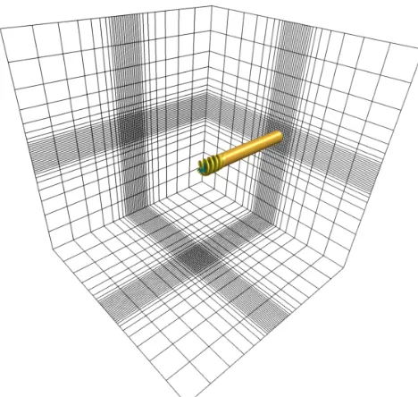
The numerical domain for the rotor simulations is dis-cretized in a verified, standard manner (Meyer Forsting et al., 2017; Troldborg et al., 2009). It consists of a box with 25R
side length that contains an inner box with a uniformly spaced refined mesh of 3.2R edge length at its centre sur-rounding the rotor (see Fig. 2). To capture the velocity gra-dients around the AL correctly the mesh spacing is 1x=
R/40. This is twice the recommended minimum (Troldborg et al., 2009); however, it delivers more accurate angle of at-tack estimates at the section centres (Shives and Crawford, 2013). In total, 256 cells discretize the flow domain along each dimension, resulting in 16.8×10⁶degrees of freedom. All variables, except pressure and its correction, which
Figure 2.Numerical box domain with a structured mesh and uni-form spacing around the rotor at its centre. Only every eighth grid point is shown.
cessitate special treatment (Sørensen, 1995), obey symmetry conditions on the lateral boundaries, whereas at the inflow and outflow faces they follow Dirichlet and Neumann condi-tions, respectively. The wing test cases follow the same ap-proach only withNs=32 and an inner box edge length of 3b, wherebis the wing’s half-span. This results in 80 cells along each dimension and 5.1×10⁵degrees of freedom. To ensure that the blade tip remains inside a single cell during one time step1t < 1x/(R) – with mesh spacing1xand rotational speed . Without rotation, the termR is replaced by the advection speed of the wake. The kinematic viscosity and air density are kept constant at 1.789×10⁻⁵kg m−1s−1and 1.225 kg m−3, respectively. Simulations are stopped when the thrust residual reaches 1×10⁻⁵.
The sensitivity of the rotor thrust to the domain size, time step and grid size is explored in Fig. 3. The length of the do-main edges is doubled to 50R, the time step is halved with respect to a set-up obeying the method described above. A simulation of the NREL 5-MW at 8 m s−1 with either 40 or 60 grid cells along the rotor depending on the smearing length scale acts as a reference. With =R/10 andR/20, this represents 4 and 3 times the recommended resolution, respectively (Troldborg et al., 2009). Although non-zero, the sensitivity of the results is acceptable in code comparison and should impact AL simulations with and without correction similarly.
3.2 Free-wake lifting line rotor simulations
The in-house solver MIRAS has been employed to perform the free-wake lifting line simulations. MIRAS is a
multi-Figure 3.Thrust sensitivity of the NREL 5-MW AL simulations at a 8 m s−1wind speed with respect to grid size, doubling the domain size and halving the time step at two smearing length scales (Ns=
{9,19},Tref= {4.20,4.06} ×105N).
fidelity computational vortex model, which is mainly used for predicting the aerodynamic behaviour of wind turbines and their wakes. It has been developed at DTU over the last decade and been extensively validated for small to large size wind turbine rotors by Ramos-García et al. (2017, 2014a, b). The free-wake vortex method essentially models the wake of a wind turbine using a bundle of infinitely thin vortex fila-ments. To avoid numerical singularities, a viscous core must be introduced, which represents a more physical distribution of the velocities induced by each vortex filament, desingular-izing the Biot–Savart law near the centre of the filament. The velocity induced by each one of the elements is obtained di-rectly by evaluating the Biot–Savart law, and by summing the velocity induced by all filaments, the total wake induction is obtained as follows:
u(xi)= N X
j=1
Kij γj
4π
tj×rij
rij3 ,
where Kij=
rij2
ε2jz+rij2z1/z
, (12)
N is total number of filaments that form the wake, rij=
xi−yj is the distance vector from the vortex elementyj
to the evaluation point xi, γj is the circulation of the
fil-ament,tj is the unit orientation vector of the jth filament
andrij= |rij|,εj is the vortex core radius of the filament,
andzdefines the cut-off velocity profile where the Lamb– Oseen model (Lamb, 1932; Oseen, 1911),z=2, has been employed.
A viscous core model is applied to emulate the effect of viscosity by changing the vortex core radius as a function of time (Leishman et al., 2002):
εi(t)=p4αvδvνti+ε0, (13)
whereαvis a constant set to 1.25643 (Ananthan and
Leish-man, 2004), ν is the kinematic viscosity andti is the time
represent the diffusive timescales, the viscous core radius is set to change with the vortex age by adding a turbulence eddy viscosity, δv, first proposed by Squire (1965), and in this work set to 1×10⁻³. To avoid the singular behaviour of newly released vortex elements, an initial core radius,ε0, is introduced. In accordance with Ramos-García et al. (2017), who found that a small core radius is necessary to have flow convergence, a core radius of 0.1 % of the local chord at the release station is used.
For the sake of the present study, two different approaches to compute the angle of attack have been followed.
– Inviscid (LL), where the non-regularized Biot–Savart law is used to compute the induction from the wake fila-ments at the quarter-chord location. This is the standard method used in a lifting line solvers.
– Viscous (LL+core), where the regularized Biot–Savart law is used to compute the induction at the quarter-chord location. A viscous core with a radius equal to the actuator line smearing factor is used for a direct compar-ison of the methods.
This enables a double validation of the models. On the one hand the corrected AL simulations can be validated against the LL calculations, and on the other hand the raw AL model, without tip correction, can be compared against the LL+core simulations which include the smearing effect in the free-wake model.
4 Tip/smearing correction for the actuator line
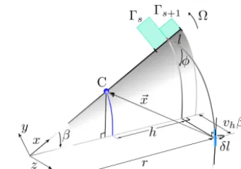
Applying the velocity correction methodology introduced in Sect. 1.1 in three-dimensional space yields a velocity correc-tion vector. The viscous core behaviour of the AL bound vor-ticity – proven in Sect. 2 to originate from the force smearing – is inherited by the trailing vortices, as will be demonstrated in Sect. 5.1.1. Therefore, the induction from the trailed vor-ticity at the blade is lower than without force smearing. Fig-ure 4 shows the path of trailed vorticity shed from in-between two sections of a blade with a strength of10=0s−0s+1 with
0s=
1 2
q v2
s+w2sCL(α)c. (14)
Heresdefines the blade section index,CLis the sectional lift coefficient,cis the section chord andαis the angle of attack, which depends on the inflow angle in combination with blade pitch and twist at the section. The missing induction from this single trailed vortex at a point C is obtained by integrating along the vortex line
u∗= ∞ Z
0
fδeudl, (15)
Figure 4.Trailed vorticity path. The blade rotates in thex−yplane andzpoints downstream. The vortex elementδlwith a strength of 0s−0s+1is shed atr and transported downstream by the local velocity. The distance from the shedding locationr to a pointC along the blade ish(h=r−Cx), whereδlinduces tangential and
axial velocities.
wherel is the vortex following coordinate. Hereδeuis the velocity induced by an infinitesimal elementδlof the vortex line at pointC, which is given by the Biot–Savart law:
δeu=10 4π
δl×x
|x|3 , (16)
wherexis the vector pointing from the element towardsC. The smearing factor for this vortex element becomes
f=exp
−(xeˆ⊥) 2
2
. (17)
The viscous core only acts in the plane orthogonal to the vor-tex elementδl; hence, eˆ⊥ projects x onto this plane. This is different to using the distance,|x|, as Dag et al. (2017) proposed, which violates the two-dimensional nature of the viscous core.
The total missing induction at a blade sectionsis obtained by summing the contribution from all trailed vortices. The number of trailed vorticesNvis directly related to the num-ber of blade sectionsNv=Ns+1. Discretizing the vortices in time, the missing induction at a certain blade section be-comes
u∗s =
Nv
X
v Nt
X
n
fs,vn 1euns,v. (18)
Here v denotes the trailed vortex index, n is the time in-dex andNt is the number of time steps. Note thatn=1 is the most recently shed vortex element. As a tip/smearing correction should remain computationally inexpensive, nu-merically solving the Biot–Savart law in Eq. (16) to ob-tain1euns,v is unfeasible. This would necessitateNtNvNs or Nt(Ns+1)Nsevaluations. An accurate, yet fast, alternative to
for dynamic flow cases and exhibits great numerical stabil-ity, as it was originally developed to enhance the aerody-namic accuracy of blade element momentum (BEM) mod-els. Its formulation is based on a lifting line representation of the blade’s trailed vorticity as depicted in Fig. 4 and approxi-mates the induced velocities from a single trailed vortex line by two indicial functions. The velocity induced by a vortex element is given in the NWM as
1euns,v= Xs,vn +Ys,vn
0 sin(φn) −cos(φn)
, (19)
withφ representing the helix angle of the vorticity shed in the CFD domain (see Fig. 4). The indicial functions take the following form:
Xns,v, Ys,vn =a{X,Y} rv
4π hs|hs|
10nvφs,v∗n
"
1−exp −b{X,Y} 1β∗n
φ∗n
s,v !#
exp −b{X,Y} n−1
X
i 1β∗i
φ∗i
s,v !
. (20)
The definitions ofa{X,Y}, b{X,Y}, β∗andφ∗are those of Pir-rung et al. (2016, 2017b). The indicial functions allow for the solution to be time-advanced by a mere multiplication, considerably reducing the model evaluations toNvNs+Nv.
In the original formulation this removes the need for book-keeping; however, as the smearing factor also changes with the position of the vortex element, all previously shed ele-ments are advanced individually in this specific implemen-tation. This is only an experimental feature for testing the smearing correction and should be simple to remove in a fu-ture, more practical implementation.
Following the lifting line formulation of the NWM shown in Fig. 4 (refer to Appendix A for a detailed mathematical de-scription) the perpendicular distance from the vortex element toCbecomes
x⊥= δl |δl|×x=
rcosφ
tanφ(βcosβ−sinβ) −tanφ(−1+h/r+cosβ+βsinβ)
−1+(1−h/r) cosβ
. (21)
Thus, the smearing factor becomes
fs,vn =exp
−|x⊥(rv, β
n, h s, φn)|2 2
. (22)
When discretizing in time,βnis taken to be at the mid-point of the vortex element.
Finally the missing velocities computed in Eq. (18) correct the original velocities from the CFD simulations
us =uCFDs +u ∗
s. (23)
Therefore, the correction influences the blade forces through the angle of attack and the velocity magnitude, although it is the former that dominates. It also changes the circulation at each blade section through Eq. (14) and, thus, the shed vorticity and its induction. Hence determining the correction velocity is an iterative procedure. The correction algorithm is executed after the flow field is solved and takes the following form:
1. Interpolate the velocity vectoruCFDat the section cen-tres from the CFD flow field.
2. Compute the helix angles φ, where φv=
−tan−1
wCFD
v−1+wvCFD
vCFDv−1+vCFD
v
andφ{1,Nv}= −tan
−1
w{CFD1,Ns}
vCFD{1,Ns}
.
3. Combine the CFD velocities with the respective cor-rection from the previous time step n−1, such that un=uCFD
n +u∗n−1.
4. Compute the smearing factorf for all time steps, sec-tions and elements (Eq. 22).
5. Determine the angle of attack and velocity magnitude fromunto determine0s (Eq. 14)3,
6. Compute the velocities from the newly released vortex element1eun(Eq. 19).
7. At the first iteration of each time step, advance the pre-vious elements in time.
8. Compute the velocity correction at the current time step u∗n(Eq. 18).
9. Update the velocity at the sections with some form of relaxationun=uCFDn +u∗n.
10. Repeat steps 5–9 until convergence is reached.
We use the technique by Pirrung et al. (2017a) established for the NWM to accelerate and ensure its convergence. Fur-thermore, the activation of the correction is delayed until the starting vorticity of the rotor has been transported at least one blade length away from the rotor plane. This enhances its numerical stability, as induction has already built up at the blades by its time of activation.
5 Results
5.1 Basic wing test cases
To verify the smearing hypothesis (Sect. 1.1) and the novel smearing correction (Sect. 4) two basic wing flow cases with known theoretical solutions are modelled using CFD. Either
Figure 5.Definition of the wing test cases with either a rectangular or elliptic planform. Vortices are trailed in-between sections and the actuator line forces are computed and exerted at the sections’ centres.
Table 1.Input parameters common to both rectangular and elliptic wing simulations.
w∞(m s−1) 2b(m) rv=1(m) (rad s−1)
10 10 0.5 0
a rectangular or an elliptic wing is represented by an AL as shown in Fig. 5, where the coordinate system is unchanged from the definition in Fig. 4. The AL is discretized in uni-formly spaced sections in-line with the underlying flow grid, and the smearing parameter is twice the section width, which ensures a continuous force distribution along the wing. The common simulation parameters are given in Table 1. Unless specifically stated the sectional lift coefficient CL=1 and drag is zero along the wing, independent of the angle of at-tack. The chord of the rectangular wing is set to 1 m and the elliptical chord distribution is
c(x)=c0
s
1−
x−(b+r v=1)
b
2
, (24)
with the root chordc0=4 m. All simulations are performed within the same computational domain, defined in Sect. 3.1. The theoretical predictions of the velocity field are achieved by representing the vortex system of Fig. 5 with vortex filaments. The velocity induced by a filament with a viscous vortex core at an arbitrary pointCis
u=f(x⊥) 0
4π
(x1+x2)(x1×x2) x1x2+x1·x2
(25)
x⊥=
|x1×x2|
|x2−x1|
and xi= |xi|, (26)
wherex1points from the start of the filament to C andx2 from its end. For a definition of f(x⊥) refer to Eq. (17); without viscous coref(x⊥)=1. The contribution from dif-ferent segments is summed to give the overall velocity field. As the wing is lightly loaded, we assume that all vortex seg-ments remain in thex−zplane.
5.1.1 Trailed vorticity smearing
The vortex smearing hypothesis assumes the trailed vortic-ity inheriting the smeared velocvortic-ity field from the bound
vor-Figure 6.Velocities induced perpendicular to a rectangular wing predicted by an actuator line (AL) without correction and by vor-tex segments with a viscous core (Vorvor-tex) with different smearing parameters. Velocities are shown along lines cutting the bound and trailed vortices at right angles andy=0. Only half of the horseshoe vortex is depicted asx0=x−(b+rv=1).
tex, which was confirmed theoretically by Martínez-Tossas and Meneveau (2019) for straight wings. We test this further by simulating a rectangular wing without any correction. All vorticity is shed from the wing tips, creating the well-known horseshoe vortex. Hence, for the hypothesis to be valid, the velocity distribution in the plane orthogonal to the trailed vortices should be identical to that of the bound vortex .
Figure 6 compares the velocities induced by a rectangu-lar wing predicted by an AL and three vortex segments (one bound, two trailed) for five different smearing parameters. Only half of the wing is presented, due to symmetry. Veloc-ity distributions are shown for lines cutting the vortex seg-ments at right angles fory=0. Clearly the velocity smear-ing is identical between trailed and bound vorticity, confirm-ing the smearconfirm-ing hypothesis. Slight differences are linked to the numerical discretization of the Gaussian force projection (Shives and Crawford, 2013) and numerical diffusion.
5.1.2 Smearing correction verification
Fig-Figure 7.Analytical (An.) and corresponding model prediction of the velocity correction for varying force smearing (=2b/(Nv−1))
along a rectangular and elliptic wing, wherex0=x−(b+rv=1).
ure 7 compares the velocity correction predicted by the ana-lytical vortex segments and our model at each section along a rectangular and elliptic wing for different smearing factors (i.e. =2b/(Nv−1)). With decreasing force smearing the velocity correction concentrates towards the tips, as the in-duced velocity gradients increase. Therefore, even at higher resolution the smearing correction remains significant, al-though more localized. Generally the model slightly over-predicts the missing induction at the wing, becoming more prominent with increasing resolution. AtNv=64 the
differ-ence reaches a maximum of 6.7 % (rectangular) and 1.7 % (elliptic) with respect to the inflow velocity. The average er-ror does not breach 0.5 % in any case. The velocity jump towards the tip sections of the elliptical wing is related to the equidistant discretization of the wing (Pirrung et al., 2014).
5.1.3 Coupled AL-smearing correction verification The coupling between velocity correction and the flow do-main is verified by comparing the corrected downwash at an elliptical wing to the theoretical expectation. The downwash should be constant along the wing and is given by
vth= −
00 4b = −
w∞c0CL
8b , (27)
where 00 is the circulation at the wing root. Similar to Shives and Crawford (2013) the CL was not fixed, but in-stead followed the theoretical lift curve slope for thin airfoils
CL=2π. For the wing to operate at a constant lift coefficient
CL=1, its angle of attack needed to include the effect of the induced velocities:
α=αeff+αi=
CL 2π +tan
−1
c
0CL 8b
. (28)
This represents a more rigorous test of the coupled system than prescribing the loading along the wing, as only the cor-rect downwash leads to the desired, constant sectional lift coefficients.
Figure 8 shows the downwash predicted by AL simu-lations with different smearing parameters and active cor-rection. The CFD components of the velocities are shown
Figure 8.Downwash at an elliptical wing predicted by AL simula-tions with different smearing factors and smearing correction. The CFD components of the velocities are shown (dashed) as well as the total downwash incorporating the correction (solid). The theoretical value acts as reference.
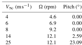
Table 2.Input parameters for the NREL 5-MW simulations.
V∞(m s−1) (rpm) Pitch (◦)
4 4.6 0.00
6 6.9 0.00
8 9.2 0.00
14 12.1 2.59 25 12.1 23.09
(vCFD) separately to emphasize the contribution of the cor-rection to arrive at the correct, constant downwash of 1 m s−1. Clearly without the correction, the induced velocities are a function of the smearing factor and only arrive at the theo-retically expected value forNv=32. Including the correc-tion greatly reduces the dependence of the downwash on the force smearing. The insufficient correction towards the tips feeds back to the equidistant discretization of the AL (Pir-rung et al., 2014), which is linked to the uniform spacing of the underlying flow grid.
5.2 Rotor simulations – NREL 5-MW
The validity of the smearing hypothesis and its correction in rotor applications is demonstrated with simulations of the NREL 5-MW turbine (Jonkman et al., 2009) using actuator line (AL) and lifting line (LL) models. The input parameters for these simulations are given in Table 2.
5.2.1 Uniform inflow
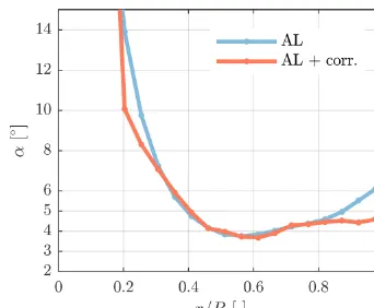
equiva-Figure 9.Normal and tangential forces on the NREL 5-MW blades at 8 m s−1predicted by AL simulations with/without smearing cor-rection and LL with/without viscous core (Ns=19,=0.1R).
lence between the original AL and the LL with a viscous core and the corrected AL with the LL. Therefore, the smearing correction makes the AL effectively act as a LL, as originally intended by Sørensen and Shen (2002). The impact of the viscous core is most prominent toward the blade root and tip. The sudden drop in the forces predicted by the AL/LL+core for the tip section of the blade – located atr/R=0.97 – is not triggered by any aerodynamic tip effects, but relates to a pronounced reduction in chord. Figure 10 shows the di-minishing effect of the correction on the angle of attack to-wards the root and tip. As the correction velocities are neg-ligible with respect to the rotational velocity – they impact the velocity magnitude by less than 0.1 % in the lifting re-gion of the blade – it is ultimately the change in the angle of attack that explains the observations in the force distribu-tions. While not greatly affecting the magnitude of the forces in the mid-section of the blade, the viscous core does intro-duce greater fluctuations in the force distribution. Hence, the missing induction introduced by the viscous core reduces the coupling between neighbouring blade sections. The smear-ing correction also recovers this behaviour of the LL. Sur-passing rated wind speed, forces increase inboard until cut-out. Thus, just before cut-out at 25 ms−1loading reaches a maximum towards the root, causing an equally pronounced influence of the smearing correction in this region, as demon-strated in Fig. 11. Again, the equivalence of the AL and LL implementations is remarkable. This high wind speed case also demonstrates our correction is not only a tip correction. The comparison of AL and LL is summarized in Fig. 12 in the form of local thrust and power distributions at differ-ent wind speeds. Note that for the wind speeds below rated (<11.4 m s−1), the coefficients are identical. The results are only presented for simulations withNs=9 for visibility, but compare equally well at higher resolution. As mentioned ear-lier, the smearing correction predominantly acts towards the tip and root. An additional overview of all results is given in Table 3. Here the total rotor thrustT and powerP predicted by the corrected actuator line (AL∗) and the lifting line (LL) are listed as well as the influence of adding the viscous core relative to AL∗and LL, respectively. The AL and LL
solu-Figure 10.Angle of attack with/without smearing correction on the NREL 5-MW blades at 8 m s−1(Ns=19,=0.1R).
Figure 11. Normal and tangential forces on the NREL 5-MW blades at 25 m s−1predicted by AL simulations with/without smear-ing correction and LL with/without viscous core (Ns=9, =
0.2R).
tions are not directly compared to avoid including any mean bias in the comparison. The impact of the correction on the AL forces is nearly identical to removing the viscous core in the LL simulations at any wind speed, which further sup-ports our correction methodology. In light of the large errors incurred without any correction, unsurprisingly, some form of tip correction is usually applied in AL simulations.
5.2.2 Yawed inflow
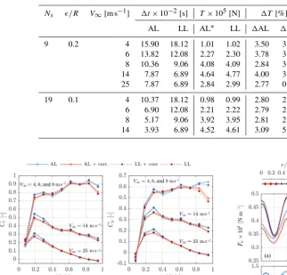
hint-Table 3. An overview of the simulation inputs and results for the NREL 5-MW in uniform inflow. Results are grouped by blade/grid resolution. For the actuator line (AL) and lifting line (LL) the simulation time step1t, the total thrustT and powerP as well as the relative change in these quantities caused by the correction/removing the viscous core are listed. Note that AL∗represents the corrected AL results, and the change is expressed relative to the rotor thrust and power.
Ns /R V∞[m s−1] 1t×10−2[s] T×105[N] 1T [%] P×106[W] 1P [%]
AL LL AL∗ LL 1AL 1LL AL∗ LL 1AL 1LL 9 0.2 4 15.90 18.12 1.01 1.02 3.50 3.21 0.26 0.26 9.19 8.74 6 13.82 12.08 2.27 2.30 3.78 3.20 0.89 0.88 8.91 8.72 8 10.36 9.06 4.08 4.09 2.84 3.20 2.13 2.08 7.51 8.71 14 7.87 6.89 4.64 4.77 4.00 3.19 5.39 5.54 5.64 4.90 25 7.87 6.89 2.84 2.99 2.77 0.82 5.40 5.68 3.08 1.65 19 0.1 4 10.37 18.12 0.98 0.99 2.80 2.13 0.25 0.25 7.48 5.81 6 6.90 12.08 2.21 2.22 2.79 2.12 0.83 0.85 7.45 5.79 8 5.17 9.06 3.92 3.95 2.81 2.13 1.98 2.02 7.49 5.81 14 3.93 6.89 4.52 4.61 3.09 5.98 5.22 5.35 4.71 7.50
Figure 12.Local thrust and power coefficients along the NREL 5-MW blades at different wind speeds predicted by AL simulations with/without smearing correction and LL with/without core (Ns=
9,=0.2R).
ing at the AL experiencing higher induction in this region. However, for the verification of the smearing correction this shift is irrelevant, instead its impact on the AL forces needs to be assessed relative to the difference between LL with and without core. In this respect the smearing correction behaves correctly, increasing forces in a similar fashion as a LL with-out core in the mid-section of the blade and reducing them towards the root and tip.
5.2.3 Pitch step
The pitch step is defined as
ψ=ψ0+
1ψ
2 [1+tanh(k(t−t0))], (29) with ψ0 defining the pitch angle before the step, t0 repre-senting the time instant of the step and 1ψ denoting the pitch change. Here an extremely violent step is chosen – de-termined byk – to encourage an equally pronounced blade
Figure 13.Normal(a, b, c)and tangential(d, e, f)force variation during one rotation as a function of azimuthal position of the NREL 5-MW blades at 8 m s−1and 45◦yaw. The forces are averaged over three sections (inner:a, d; middle:b, e; outer:c, f) of the blade and are predicted by AL simulations with/without smearing correction and LL with/without viscous core. The blade is facing upwind at χ=0◦and is pointing vertically up atχ=90◦(Ns=9,=0.2R).
force response and test the numerical stability of our correc-tion. The parameters governing this comparison are given in Table 4, which realize a pitch step of±2◦ in 0.14 s (10 % to 90 % pitch). To capture the swift change in pitch, the time step is adjusted in both AL and LL simulations to 3.94×10⁻²s. The blade force response is normalized as
ˆ
F(t)=F(t)−F0
F∞−F0
Table 4.Inputs defining the pitch step.
V∞[m s−1] [rpm] ψ0[◦] 1ψ[◦] k 14 12.1 2.59 ±2 16
Figure 14.Normalized tangential force response at two blade sec-tions (middle and tip) of the NREL 5-MW following a pitch step of
+2◦in 0.14 s at 14 m s−1predicted by AL simulations with/without smearing correction and LL with/without viscous core (Ns=9, =0.2R).
withF0andF∞denoting the steady-state values before and after the pitch step, respectively.
Here only the tangential force response after a +2◦ step for the mid and tip blade sections are shown in Fig. 14, as they capture the main features of the response. As the defini-tion here is positive pitch to feather, the force decreases along the blade for positive pitch changes. The AL simulations ex-hibit a faster response with a kink at 0.14 s, coinciding with the pitch change reaching 99 % of the step. Therefore, the AL seems to capture the pitch rate lift. The LL does not show this feature so – as in yaw – the correct behaviour of the smear-ing correction on the AL force response should be assessed relative to the influence of removing the viscous core in the LL model. Overall, the correction has limited effect on the dynamic response, which is also confirmed by the LL sim-ulations, but the correction essentially acts on the forces in the same fashion as removing the core in the LL. In the mid-section it reduces the forces by a maximum of 1 % during the first 2 s, dropping to 0.5 % afterwards. At the tip section it intensifies the response by a maximum of 1 %, diminishing to 0.3 % at 4 s.
5.2.4 Turbulent inflow
Highly turbulent inflow should challenge the numerical sta-bility of the new smearing correction by introducing strong and abrupt changes in the angle of attack. Comparing sim-ulations with and without inflow turbulence should also re-veal whether turbulence alters the nature of the correction. Figure 15 shows the impact of the smearing correction on the time-averaged normal and tangential blade forces at an 8 m s−1mean wind speed for AL simulations with uniform and turbulent inflow. At a turbulence intensity (TI) of 15 %,
Figure 15. Time-averaged normal and tangential forces on the NREL 5-MW blades at an 8 m s−1mean wind speed and chang-ing inflow turbulence predicted by the AL model with and without smearing correction (Ns=35,=R/8).
Figure 16.Variation of normal and tangential forces on the NREL 5-MW blades at an 8 m s−1mean wind speed and turbulence inten-sity of 15 % predicted by the AL model with and without smearing correction (Ns=35,=R/8).
the forces are unsurprisingly slightly larger (≈20 N m−1) than in uniform inflow. However, the change in forces in-troduced by the correction is nearly identical (<2 N m−1). When comparing the standard deviation of the forces with and without correction in Fig. 16 the smoothing and damp-ening effect of the smearing correction on the forces in highly turbulent inflow also becomes apparent. Madsen et al. (2018) observed a corresponding reduction of the force variations on the whole rotor blade when comparing near-wake model re-sults against BEM rere-sults for the NM 80 rotor in turbulent inflow. This illustrates that the smearing correction leads to the same dynamic coupling between neighbouring blade sec-tions as a lifting line model.
6 Conclusions
an actuator line induces lower velocities at the blade owing to the force projection. We recover this missing induction by combining a near-wake model of the trailed vorticity with the Lamb–Oseen viscous core model and coupling it with the ac-tuator line model. Basic wing test cases with theoretical solu-tions verify the correction, as it recovers nearly all induction independent of the severity of the force smearing. Further-more, rotor simulations show the applicability and strength of the correction over the entire operational wind speed range as well as in yaw, strong turbulence and undergoing pitch steps. Here the correction is validated with lifting line simu-lations with and without viscous core, which are representa-tive of an actuator line with and without smearing correction, respectively. The agreement between the respective actuator line and lifting line results is remarkable.
The current implementation of the smearing correction re-lies on heavy bookkeeping. In future versions the latter will be removed without jeopardizing stability or accuracy, mak-ing it suitable for wind farm simulations in realistic atmo-spheric flows. Potentially, the correction might also enable accurate rotor simulations at lower discretization.
Appendix A: Fixed-wake equations
The equations governing the fixed-wake approach underly-ing the smearunderly-ing correction (see Fig. 4) are summarized for completeness.
Direction vector from the vortex element to a control point along the blade:
x=
−rcosβ+r−h rsinβ
−vhβ/
. (A1)
Definition of the vortex element:
δl=δlcosφ
−sinβ
−cosβ vh/(r)
(A2)
withδl= rδβ
cosφ. Note that
cosφ= r
q
(r)2+v2h
= 1
q
1+ vh
r 2
(A3)
with tanφ= vh
r.
Incremental velocity induced by the vortex element
δeu=10 4π
δl×x |x|3 =
Ar
(vh/ r) (βcosβ−sinβ)
−(vh/ r) (−1+hr+cosβ+βsinβ)
[−1+(1−hr) cosβ]
, (A4)
with
A=10rδβ 4π
"
r2 1+(1−hr)2−2 (1−hr) cosβ+
v hβ r
2!#
| {z }
|x|2
−3 2
hr= h
Author contributions. ARMF was responsible for writing the pa-per, except for Sect. 3.2 which was authored by NRG. The origi-nal numerical implementation of the near-wake model by GRP was adapted by ARMF to incorporate the smearing correction with the help of GRP. NRG performed all simulations with the lifting line, and ARMF performed all simulations with the actuator line. All au-thors decided on the flow cases to simulate and commented on the paper.
Competing interests. The authors declare that they have no con-flict of interest.
Acknowledgements. We would like to acknowledge DTU Wind Energy’s internal project “Virtual Atmosphere” for partially fund-ing this research. Furthermore many thanks to senior researcher Mac Gaunaa for his insights on vortex aerodynamics and senior researcher Niels Troldborg for his input on actuator line simula-tions/modelling (both from DTU Wind Energy). Thanks also to Ang Li for his help regarding the near-wake model.
Review statement. This paper was edited by Alessandro Bian-chini and reviewed by two anonymous referees.
References
Ananthan, S. and Leishman, J. G.: Role of Filament Strain in the Free-Vortex Modeling of Rotor Wakes, J. Am. Helicopter Soc., 9, 176–191, 2004.
Dag, K., Sørensen, J., Sørensen, N., and Shen, W.: Combined pseudo-spectral/actuator line model for wind turbine applica-tions, PhD thesis, DTU Wind Energy, Denmark, 2017.
Forsythe, J. R., Lynch, E., Polsky, S., and Spalart, P.: Coupled Flight Simulator and CFD Calculations of Ship Airwake using Kestrel, in: 53rd AIAA Aerospace Sciences Meeting, AIAA, Kissimmee, Florida, USA, https://doi.org/10.2514/6.2015-0556, 2015. Glauert, H.: Airplane Propellers, Springer Berlin Heidelberg,
Berlin, Heidelberg, 169–360, https://doi.org/10.1007/978-3-642-91487-4_3, 1935.
Jha, P. K., Churchfield, M. J., Moriarty, P. J., and Schmitz, S.: Guidelines for Volume Force Distributions Within Ac-tuator Line Modeling of Wind Turbines on Large-Eddy Simulation-Type Grids, J. Sol. Energ.-T. ASME, 136, 031003, https://doi.org/10.1115/1.4026252, 2014.
Jonkman, J., Butterfield, S., Musial, W., and Scott, G.: Definition of a 5-MW reference wind turbine for offshore system devel-opment, Tech. rep., NREL/TP-500-38060, National Renewable Energy Laboratory (NREL), Colorado, USA, 2009.
Lamb, H.: Hydrodynamics, C.U.P, 6th Edn., Cambridge University Press, Cambridge, 1932.
Leishman, J. G., Bhagwat, M. J., and Bagai, A.: Free-Vortex Fil-ament Methods for the Analysis of Helicopter Rotor Wakes, J. Aircraft, 39, 759–775, 2002.
Leonard, B.: A stable and accurate convective modelling procedure based on quadratic upstream interpolation, Comput. Method. Appl. M., 19, 59–98, 1979.
Madsen, H. A., Sørensen, N. N., Bak, C., Troldborg, N., and Pir-rung, G.: Measured aerodynamic forces on a full scale 2 MW tur-bine in comparison with EllipSys3D and HAWC2 simulations, J. Phys. Conf. Ser., 1037, 022011, https://doi.org/10.1088/1742-6596/1037/2/022011, 2018.
Martínez-Tossas, L. A. and Meneveau, C.: Filtered lifting line the-ory and application to the actuator line model, J. Fluid Mech., 863, 269–292, https://doi.org/10.1017/jfm.2018.994, 2019. Menter, F. R.: Zonal two equation k−ω turbulence models for
aerodynamic flows, in: 23rd Fluid Dynamics, Plasmadynamics, and Lasers Conference, Fluid Dynamics and Co-located Confer-ences, Orlando,FL, https://doi.org/10.2514/6.1993-2906, 1993. Meyer Forsting, A., Troldborg, N., Bechmann, A., and
Réthoré, P.-E.: Modelling Wind Turbine Inflow: The In-duction Zone, PhD thesis, DTU Wind Energy, Denmark, https://doi.org/10.11581/DTU:00000022, 2017.
Michelsen, J.: Basis3D – a platform for development of multiblock PDE solvers, Tech. rep., Dept. of Fluid Mechanics, Technical University of Denmark, DTU, 1994a.
Michelsen, J.: Block structured multigrid solution of 2D and 3D elliptic PDE’s, Tech. rep., Dept. of Fluid Mechanics, Technical University of Denmark, DTU, 1994b.
Mikkelsen, R.: Actuator Disc Methods Applied to Wind Turbines, PhD thesis, Technical University of Denmark, 2003.
Nathan, J.: Application of Actuator Surface Concept in LES Simu-lations of the Near Wake of Wind Turbines, PhD thesis, École de Technologie Supérieure, Montreal, Canada, 2018.
Oseen, C.: Über Wirbelbewegung in einer reibenden Flüssigkeit, Arkiv för matematik, astronomi och fysik, Ark. Mat. Astron. Fys., 7, 14–21, 1911.
Patanker, S. and Spalding, D.: A calculation procedure for heat, mass and momentum transfer in three-dimensional parabolic flows, Int. J. Heat Mass Tran., 15, 59–98, 1972.
Pirrung, G. R., Hansen, M. H., and Madsen, H. A.: Improvement of a near wake model for trailing vorticity, J. Phys. Conf. Ser., 555, 012083, https://doi.org/10.1088/1742-6596/555/1/012083, 2014. Pirrung, G., Madsen, H. A., Kim, T., and Heinz, J.: A coupled near and far wake model for wind turbine aerodynamics, Wind En-ergy, 19, 2053–2069, https://doi.org/10.1002/we.1969, 2016. Pirrung, G., Riziotis, V., Madsen, H., Hansen, M., and Kim,
T.: Comparison of a coupled near- and far-wake model with a free-wake vortex code, Wind Energ. Sci., 2, 15–33, https://doi.org/10.5194/wes-2-15-2017, 2017a.
Pirrung, G. R., Madsen, H. A., and Schreck, S.: Trailed vortic-ity modeling for aeroelastic wind turbine simulations in stand-still, Wind Energ. Sci., 2, 521–532, https://doi.org/10.5194/wes-2-521-2017, 2017b.
Ramos-García, N., Shen, W. Z., and Sørensen, J. N.: Val-idation of a three-dimensional viscous-inviscid interactive solver for wind turbine rotors, Renew. Energ., 70, 78–92, https://doi.org/10.1016/j.renene.2014.04.001, 2014a.
Ramos-García, N., Shen, W. Z., and Sørensen, J. N.: Three-dimensional viscous-inviscid coupling method for wind turbine computations, Wind Energy, 19, 67–93, https://doi.org/10.1002/we.1821, 2014b.
Réthoré, P.-E. and Sørensen, N.: A discrete force allocation algo-rithm for modelling wind turbines in computational fluid dynam-ics, Wind Energy, 15, 915–926, https://doi.org/10.1002/we.525, 2012.
Shen, W., Sørensen, J., and Mikkelsen, R.: Tip loss correction for actuator/Navier Stokes computations, J. Sol. Energ.-T. ASME, 59, 209–213, 2005.
Shives, M. and Crawford, C.: Mesh and load distribution require-ments for actuator line CFD simulations, Wind Energy, 16, 657– 669, https://doi.org/10.1002/we.1546, 2013.
Sørensen, J. N. and Shen, W. Z.: Numerical modelling of wind turbine wakes, J. Fluid. Eng.-T. ASME, 124, 393–399, https://doi.org/10.1115/1.1471361, 2002.
Sørensen, N.: General purpose flow solver applied to flow over hills, PhD thesis, Risø National Laboratory, 1995.
Squire, H. B.: The growth of a vortex in turbulent flow, Aeronaut. Quart., 16, 302–306, 1965.
Strelets, M.: Detached eddy simulation of massively separated flows, in: 39th AIAA Aerospace Sciences Meeting and Exhibit, AIAA Paper 2001-0879, Reno, NV, 2001.
Troldborg, N., Sørensen, J., and Mikkelsen, R.: Actuator Line Mod-eling of Wind Turbine Wakes, PhD thesis, Technical University of Denmark, 2009.