E
E
F
F
F
F
I
I
C
C
I
I
E
E
N
N
C
C
Y
Y
O
O
F
F
S
S
O
O
M
M
E
E
M
M
O
O
D
D
I
I
F
F
I
I
E
E
D
D
R
R
A
A
T
T
I
I
O
O
T
T
Y
Y
P
P
E
E
E
E
S
S
T
T
I
I
M
M
A
A
T
T
O
O
R
R
S
S
U
U
S
S
I
I
N
N
G
G
P
P
R
R
O
O
D
D
U
U
C
C
T
T
O
O
F
F
S
S
A
A
M
M
P
P
L
L
E
E
S
S
I
I
Z
Z
E
E
A
A
N
N
D
D
P
P
A
A
R
R
A
A
M
M
E
E
T
T
E
E
R
R
S
S
O
O
F
F
A
A
U
U
X
X
I
I
L
L
I
I
A
A
R
R
Y
Y
V
V
A
A
R
R
I
I
A
A
B
B
L
L
E
E
F
F
O
O
R
R
E
E
S
S
T
T
I
I
M
M
A
A
T
T
I
I
N
N
G
G
P
P
O
O
P
P
U
U
L
L
A
A
T
T
I
I
O
O
N
N
M
M
E
E
A
A
N
N
S
S
.
.
A
A
.
.
S
S
u
u
l
l
e
e
i
i
m
m
a
a
n
n
11,
,
A
A
.
.
A
A
.
.
A
A
d
d
e
e
w
w
a
a
r
r
a
a
221 Department of Statistics, Kwara State Polytechnic, Ilorin, Nigeria 2 Department of Statistics, University of Ilorin, Ilorin, Nigeria
Corresponding Author: S. A. Suleiman, [email protected]
ABSTRACT: In this paper, we modified twenty-eight ratio type estimators for estimation of population mean of the study variable earlier suggested by Gupta and Yadav ([GY17]) using product of sample size and population parameter of auxiliary variable. The expressions for the bias and mean square errors of the newly modified ratio type estimators have been obtained up to the first order of approximation. A comparison has been made with the mentioned existing ratio estimators of population mean using the same data set used by Gupta and Yadav ([GY17]) for easy justification. The results obtained on the Mean Square Errors shows that the newly modified ratio type estimators perform better vis-à-vis the earlier suggested Gupta and Yadav ([GY17]) existing ratio type estimators but the newly modified ratio type Estimator,
t*
27, perform better, hence, recommended for usage in
Sampling.
KEYWORDS: Ratio Estimator, Auxiliary information, Sample size, Bias, Mean Squared Error, Efficiency.
1. INTRODUCTION
In sample survey, the main objective is to obtain the estimators of parameters of interest with increase precision. It is common practice to use the auxiliary variable for improving the precision of the estimate of a parameter. Use of such auxiliary information is made through the ratio method of estimation to obtain an improved estimator of population mean when is highly positively correlated with variable under study. In this paper, we have modified about twenty-eight Ratio Type Estimators earlier suggested by Gupta and Yadav ([GY17]) for improved estimation of population mean with higher efficiencies.
Let the population under consideration consists of N distinct and identifiable units and let (xi,yi),
i=1,2,…,n be a two variable sample of size n taken from bivariate variable (X,Y) through simple random sampling without sampling scheme. Let 𝑋̅
and 𝑌̅ be the population means of the auxiliary and the study variable respectively, and let 𝑥̅ and 𝑦̅ be respective sample means and both unbiased estimators of 𝑋̅ and 𝑌̅ respectively. Let the
correlation coefficient between the variables X and Y be denoted by ρ ([Coc40]).
2. EXISTING ESTIMATORS UNDER REVIEW
Let the sample mean 𝑦̅ by define as:
𝑦̅ = 1
𝑛∑ 𝑦𝑖
𝑛
𝑖=1 (1)
Its variance up to the first order of approximation be:
𝑣(𝑦̅) =1−𝑓
𝑛 𝑠𝑦
2 (2)
The usual ratio estimator of population be denoted as:
𝑡𝑥= 𝑦̅ 𝑋̅
𝑥̅ (3)
Its bias and mean squared error, up to the first order of approximation respectively be:
𝐵(𝑡𝑅) = 1−𝑓
𝑛 1 𝑋̅[𝑅1𝑆𝑥
2− 𝜌𝑆
𝑦𝑆𝑥] (4)
𝑀𝑆𝐸(𝑡𝑅) = 1−𝑓
𝑛 [𝑆𝑦 2+ 𝑅
12𝑆𝑥2− 2𝑅1𝜌𝑆𝑦𝑆𝑥] (5)
Where, 𝑅1 = 𝑌̅
𝑋̅ ([Coc40, Coc77]).
Some of the earlier suggested Gupta and Yadav ([GY17]) existing Ratio Type Estimators are as shown in Table 1.
3. NEWLY MODIFIED RATIO TYPE ESTIMATORS
Motivated by the work of Gupta and Yadav ([GY17]), we have used a product of sample size and parameters of auxiliary variable given as ti*, i=1,2,…,28 as also shown in Table 1, where τ=ρ/β1
𝑦̅ = 𝑌̅(1 + 𝑒0),𝑥̅ = 𝑋̅(1 + 𝑒1),𝐸(𝑒𝑖) = 0, (𝑖 =
0,1),𝐸(𝑒02) =1−𝑓 𝑛 𝐶𝑦
2
𝐸(𝑒12) = 1−𝑓
𝑛 𝐶𝑥 2,𝐸(𝑒
0𝑒1) = 1−𝑓
𝑛 𝜌𝐶𝑦𝐶𝑥,𝑓 = 𝑛 𝑁,𝐶𝑦
2=
𝑆𝑦2
𝑌̅2,𝐶𝑥
2 =𝑆𝑥2
𝑋̅2 𝐵(𝑡𝑗∗) =
1−𝑓 𝑛
𝑆𝑥2
𝑌̅ 𝑅𝑗
∗2, (𝑗 = 2, … ,29), (6)
𝑀𝑆𝐸(𝑡𝑗∗) = 𝑛 [𝑅𝑗∗2𝑆𝑥2+ 𝑆𝑦2(1 − 𝜌2)], (𝑗 =
2, … ,29) (7)
and 𝑅𝑗∗2, (𝑗 = 2, … ,29)
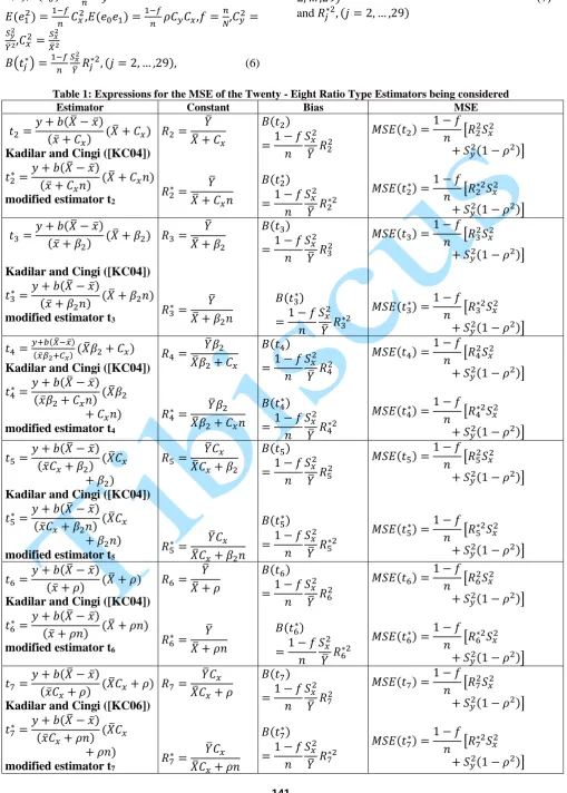
Table 1: Expressions for the MSE of the Twenty - Eight Ratio Type Estimators being considered
Estimator Constant Bias MSE
𝑡2=
𝑦 + 𝑏(𝑋̅ − 𝑥̅)
(𝑥̅ + 𝐶𝑥) (𝑋̅ + 𝐶𝑥)
Kadilar and Cingi ([KC04])
𝑡2∗ =
𝑦 + 𝑏(𝑋̅ − 𝑥̅)
(𝑥̅ + 𝐶𝑥𝑛) (𝑋̅ + 𝐶𝑥𝑛)
modified estimator t2
𝑅2=
𝑌̅ 𝑋̅ + 𝐶𝑥
𝑅2∗=
𝑌̅ 𝑋̅ + 𝐶𝑥𝑛
𝐵(𝑡2)
=1 − 𝑓 𝑛
𝑆𝑥2
𝑌̅ 𝑅2
2
𝐵(𝑡2∗)
=1 − 𝑓 𝑛
𝑆𝑥2
𝑌̅ 𝑅2
∗2
𝑀𝑆𝐸(𝑡2) =
1 − 𝑓 𝑛 [𝑅2
2𝑆 𝑥2
+ 𝑆𝑦2(1 − 𝜌2)]
𝑀𝑆𝐸(𝑡2∗) =
1 − 𝑓 𝑛 [𝑅2
∗2𝑆 𝑥2
+ 𝑆𝑦2(1 − 𝜌2)]
𝑡3=
𝑦 + 𝑏(𝑋̅ − 𝑥̅) (𝑥̅ + 𝛽2)
(𝑋̅ + 𝛽2)
Kadilar and Cingi ([KC04])
𝑡3∗ =
𝑦 + 𝑏(𝑋̅ − 𝑥̅) (𝑥̅ + 𝛽2𝑛)
(𝑋̅ + 𝛽2𝑛)
modified estimator t3
𝑅3=
𝑌̅ 𝑋̅ + 𝛽2
𝑅3∗=
𝑌̅ 𝑋̅ + 𝛽2𝑛
𝐵(𝑡3)
=1 − 𝑓 𝑛
𝑆𝑥2
𝑌̅ 𝑅3
2
𝐵(𝑡3∗)
=1 − 𝑓 𝑛
𝑆𝑥2
𝑌̅ 𝑅3
∗2
𝑀𝑆𝐸(𝑡3) =
1 − 𝑓 𝑛 [𝑅3
2𝑆 𝑥2
+ 𝑆𝑦2(1 − 𝜌2)]
𝑀𝑆𝐸(𝑡3∗) =1 − 𝑓
𝑛 [𝑅3
∗2𝑆 𝑥2
+ 𝑆𝑦2(1 − 𝜌2)]
𝑡4 =
𝑦+𝑏(𝑋̅−𝑥̅)
(𝑥̅𝛽2+𝐶𝑥)(𝑋̅𝛽2+ 𝐶𝑥)
Kadilar and Cingi ([KC04])
𝑡4∗ =
𝑦 + 𝑏(𝑋̅ − 𝑥̅) (𝑥̅𝛽2+ 𝐶𝑥𝑛)
(𝑋̅𝛽2
+ 𝐶𝑥𝑛) modified estimator t4
𝑅4=
𝑌̅𝛽2
𝑋̅𝛽2+ 𝐶𝑥
𝑅4∗=
𝑌̅𝛽2
𝑋̅𝛽2+ 𝐶𝑥𝑛
𝐵(𝑡4)
=1 − 𝑓 𝑛
𝑆𝑥2
𝑌̅ 𝑅4
2
𝐵(𝑡4∗)
=1 − 𝑓 𝑛
𝑆𝑥2
𝑌̅ 𝑅4
∗2
𝑀𝑆𝐸(𝑡4) =
1 − 𝑓 𝑛 [𝑅4
2𝑆 𝑥2
+ 𝑆𝑦2(1 − 𝜌2)]
𝑀𝑆𝐸(𝑡4∗) =
1 − 𝑓 𝑛 [𝑅4
∗2𝑆 𝑥2
+ 𝑆𝑦2(1 − 𝜌2)]
𝑡5 =
𝑦 + 𝑏(𝑋̅ − 𝑥̅) (𝑥̅𝐶𝑥+ 𝛽2)
(𝑋̅𝐶𝑥
+ 𝛽2)
Kadilar and Cingi ([KC04])
𝑡5∗ =
𝑦 + 𝑏(𝑋̅ − 𝑥̅) (𝑥̅𝐶𝑥+ 𝛽2𝑛)
(𝑋̅𝐶𝑥
+ 𝛽2𝑛) modified estimator t5
𝑅5=
𝑌̅𝐶𝑥
𝑋̅𝐶𝑥+ 𝛽2
𝑅5∗=
𝑌̅𝐶𝑥
𝑋̅𝐶𝑥+ 𝛽2𝑛
𝐵(𝑡5)
=1 − 𝑓 𝑛
𝑆𝑥2
𝑌̅ 𝑅5
2
𝐵(𝑡5∗)
=1 − 𝑓 𝑛
𝑆𝑥2
𝑌̅ 𝑅5
∗2
𝑀𝑆𝐸(𝑡5) =
1 − 𝑓 𝑛 [𝑅5
2𝑆 𝑥2
+ 𝑆𝑦2(1 − 𝜌2)]
𝑀𝑆𝐸(𝑡5∗) =
1 − 𝑓 𝑛 [𝑅5
∗2𝑆 𝑥2
+ 𝑆𝑦2(1 − 𝜌2)]
𝑡6 =
𝑦 + 𝑏(𝑋̅ − 𝑥̅)
(𝑥̅ + 𝜌) (𝑋̅ + 𝜌)
Kadilar and Cingi ([KC04])
𝑡6∗ =
𝑦 + 𝑏(𝑋̅ − 𝑥̅)
(𝑥̅ + 𝜌𝑛) (𝑋̅ + 𝜌𝑛)
modified estimator t6
𝑅6=
𝑌̅ 𝑋̅ + 𝜌
𝑅6∗=
𝑌̅ 𝑋̅ + 𝜌𝑛
𝐵(𝑡6)
=1 − 𝑓 𝑛
𝑆𝑥2
𝑌̅ 𝑅6
2
𝐵(𝑡6∗)
=1 − 𝑓 𝑛
𝑆𝑥2
𝑌̅ 𝑅6
∗2
𝑀𝑆𝐸(𝑡6) =
1 − 𝑓 𝑛 [𝑅6
2𝑆 𝑥2
+ 𝑆𝑦2(1 − 𝜌2)]
𝑀𝑆𝐸(𝑡6∗) =
1 − 𝑓 𝑛 [𝑅6
∗2𝑆 𝑥2
+ 𝑆𝑦2(1 − 𝜌2)]
𝑡7 =
𝑦 + 𝑏(𝑋̅ − 𝑥̅)
(𝑥̅𝐶𝑥+ 𝜌) (𝑋̅𝐶𝑥+ 𝜌)
Kadilar and Cingi ([KC06])
𝑡7∗ =
𝑦 + 𝑏(𝑋̅ − 𝑥̅) (𝑥̅𝐶𝑥+ 𝜌𝑛) (𝑋̅𝐶𝑥
+ 𝜌𝑛)
modified estimator t7
𝑅7=
𝑌̅𝐶𝑥
𝑋̅𝐶𝑥+ 𝜌
𝑅7∗=
𝑌̅𝐶𝑥
𝑋̅𝐶𝑥+ 𝜌𝑛
𝐵(𝑡7)
=1 − 𝑓 𝑛
𝑆𝑥2
𝑌̅ 𝑅7
2
𝐵(𝑡7∗)
=1 − 𝑓 𝑛
𝑆𝑥2
𝑌̅ 𝑅7
∗2
𝑀𝑆𝐸(𝑡7) =
1 − 𝑓 𝑛 [𝑅7
2𝑆 𝑥2
+ 𝑆𝑦2(1 − 𝜌2)]
𝑀𝑆𝐸(𝑡7∗) =
1 − 𝑓 𝑛 [𝑅7
∗2𝑆 𝑥2
Estimator Constant Bias MSE
𝑡8=
𝑦 + 𝑏(𝑋̅ − 𝑥̅) (𝑥̅𝜌 + 𝐶𝑥)
(𝑋̅𝜌 + 𝐶𝑥)
Kadilar and Cingi ([KC06])
𝑡8∗=
𝑦 + 𝑏(𝑋̅ − 𝑥̅) (𝑥̅𝜌 + 𝐶𝑥𝑛) (𝑋̅𝜌
+ 𝐶𝑥𝑛) modified estimator t8
𝑅8=
𝑌̅ 𝑋̅𝜌 + 𝐶𝑥
𝑅8∗=
𝑌̅ 𝑋̅𝜌 + 𝐶𝑥𝑛
𝐵(𝑡8)
=1 − 𝑓 𝑛
𝑆𝑥2
𝑌̅ 𝑅8
2
𝐵(𝑡8∗)
=1 − 𝑓 𝑛
𝑆𝑥2
𝑌̅ 𝑅8
∗2
𝑀𝑆𝐸(𝑡8) =
1 − 𝑓 𝑛 [𝑅8
2𝑆 𝑥2
+ 𝑆𝑦2(1 − 𝜌2)]
𝑀𝑆𝐸(𝑡8∗) =
1 − 𝑓 𝑛 [𝑅8
∗2𝑆 𝑥2
+ 𝑆𝑦2(1 − 𝜌2)]
𝑡9=
𝑦 + 𝑏(𝑋̅ − 𝑥̅) (𝑥̅𝛽2+ 𝜌)
(𝑋̅𝛽2+ 𝜌)
Kadilar and Cingi ([KC06])
𝑡9∗=
𝑦 + 𝑏(𝑋̅ − 𝑥̅)
(𝑥̅𝛽2+ 𝜌𝑛)
(𝑋̅𝛽2+ 𝜌𝑛)
modified estimator t9
𝑅9=
𝑌̅𝛽2
𝑋̅𝛽2+ 𝜌
𝑅9∗=
𝑌̅𝛽2
𝑋̅𝛽2+ 𝜌𝑛
𝐵(𝑡9) =
1 − 𝑓 𝑛
𝑆𝑥2
𝑌̅ 𝑅9
2
𝐵(𝑡9∗)
=1 − 𝑓 𝑛
𝑆𝑥2
𝑌̅ 𝑅9
∗2
𝑀𝑆𝐸(𝑡9) =
1 − 𝑓 𝑛 [𝑅9
2𝑆 𝑥2
+ 𝑆𝑦2(1 − 𝜌2)]
𝑀𝑆𝐸(𝑡9∗) =
1 − 𝑓 𝑛 [𝑅9
∗2𝑆 𝑥2
+ 𝑆𝑦2(1 − 𝜌2)]
𝑡10=
𝑦 + 𝑏(𝑋̅ − 𝑥̅)
(𝑥̅𝜌 + 𝛽2)
(𝑋̅𝜌 + 𝛽2)
Kadilar and Cingi ([KC06])
𝑡10∗ =
𝑦 + 𝑏(𝑋̅ − 𝑥̅) (𝑥̅ 𝜌 + 𝛽2𝑛)
(𝑋̅𝜌
+ 𝛽2𝑛) modified estimator t10
𝑅10 =
𝑌̅𝜌 𝑋̅𝜌 + 𝛽2
𝑅10∗ = 𝑌̅𝜌
𝑋̅𝜌 + 𝛽2𝑛
𝐵(𝑡10)
=1 − 𝑓 𝑛
𝑆𝑥2
𝑌̅ 𝑅10
2
𝐵(𝑡10∗ )
=1 − 𝑓 𝑛
𝑆𝑥2
𝑌̅ 𝑅10
∗2
𝑀𝑆𝐸(𝑡10) =
1 − 𝑓 𝑛 [𝑅10
2 𝑆 𝑥2
+ 𝑆𝑦2(1 − 𝜌2)]
𝑀𝑆𝐸(𝑡10∗ ) =1 − 𝑓
𝑛 [𝑅10
∗2𝑆 𝑥2
+ 𝑆𝑦2(1 − 𝜌2)]
𝑡11=
𝑦 + 𝑏(𝑋̅ − 𝑥̅)
(𝑥̅ + 𝛽1) (𝑋̅ + 𝛽1)
Yan and Tian ([YT10])
𝑡11∗ =
𝑦 + 𝑏(𝑋̅ − 𝑥̅) (𝑥̅ +𝛽1𝑛) (𝑋̅
+ 𝛽1𝑛) modified estimator t11
𝑅11 =
𝑌̅ 𝑋̅ + 𝛽1
𝑅11∗ =
𝑌̅ 𝑋̅ + 𝛽1𝑛
𝐵(𝑡11)
=1 − 𝑓 𝑛
𝑆𝑥2
𝑌̅ 𝑅11
2
𝐵(𝑡11∗ )
=1 − 𝑓 𝑛
𝑆𝑥2
𝑌̅ 𝑅11
∗2
𝑀𝑆𝐸(𝑡11) =
1 − 𝑓 𝑛 [𝑅11
2 𝑆 𝑥2
+ 𝑆𝑦2(1 − 𝜌2)]
𝑀𝑆𝐸(𝑡11∗ ) =
1 − 𝑓 𝑛 [𝑅11
∗2𝑆 𝑥2
+ 𝑆𝑦2(1 − 𝜌2)]
𝑡12=
𝑦 + 𝑏(𝑋̅ − 𝑥̅)
(𝑥̅𝛽1+ 𝛽2)
(𝑋̅𝛽1+ 𝛽2)
Yan and Tian ([YT10])
𝑡12∗ =𝑦 + 𝑏(𝑋̅ − 𝑥̅)
(𝑥̅ 𝛽1+ 𝛽2𝑛)
(𝑋̅𝛽1
+ 𝛽2𝑛) modified estimator t12
𝑅12 =
𝑌̅𝛽1
𝑋̅𝛽1+ 𝛽2
𝑅12∗ =
𝑌̅𝛽1
𝑋̅𝛽1+ 𝛽2𝑛
𝐵(𝑡12)
=1 − 𝑓 𝑛
𝑆𝑥2
𝑌̅ 𝑅12
2
𝐵(𝑡12∗ )
=1 − 𝑓 𝑛
𝑆𝑥2
𝑌̅ 𝑅12
∗2
𝑀𝑆𝐸(𝑡12) =
1 − 𝑓 𝑛 [𝑅12
2 𝑆 𝑥2
+ 𝑆𝑦2(1 − 𝜌2)]
𝑀𝑆𝐸(𝑡12∗ ) =1 − 𝑓
𝑛 [𝑅12
∗2𝑆 𝑥2
+ 𝑆𝑦2(1 − 𝜌2)]
𝑡13=
𝑦 + 𝑏(𝑋̅ − 𝑥̅)
(𝑥̅ + 𝑀𝑑)
(𝑋̅ + 𝑀𝑑)
Subramani and
Kumarpandiyan ([SJ12])
𝑡13∗ =
𝑦 + 𝑏(𝑋̅ − 𝑥̅)
(𝑥̅ + 𝑀𝑑𝑛)
(𝑋̅ + 𝑀𝑑𝑛)
modified estimator t13
𝑅13 =
𝑌̅ 𝑋̅ + 𝑀𝑑
𝑅13∗ =
𝑌̅ 𝑋̅ + 𝑀𝑑𝑛
𝐵(𝑡13)
=1 − 𝑓 𝑛
𝑆𝑥2
𝑌̅ 𝑅13
2
𝐵(𝑡13∗ )
=1 − 𝑓 𝑛
𝑆𝑥2
𝑌̅ 𝑅13
∗2
𝑀𝑆𝐸(𝑡13) =
1 − 𝑓 𝑛 [𝑅13
2 𝑆 𝑥2
+ 𝑆𝑦2(1 − 𝜌2)]
𝑀𝑆𝐸(𝑡13∗ ) =
1 − 𝑓 𝑛 [𝑅13
∗2𝑆 𝑥2
+ 𝑆𝑦2(1 − 𝜌2)]
𝑡14=
𝑦 + 𝑏(𝑋̅ − 𝑥̅)
(𝑥̅𝐶𝑥+ 𝑀𝑑)
(𝑋̅𝐶𝑥+ 𝑀𝑑)
Subramani and
Kumarpandiyan ([SJ12])
𝑡14∗ =
𝑦 + 𝑏(𝑋̅ − 𝑥̅) (𝑥̅𝐶𝑥+ 𝑀𝑑𝑛)
(𝑋̅𝐶𝑥
+ 𝑀𝑑𝑛) modified estimator t14
𝑅14=
𝑌̅𝐶𝑥
𝑋̅𝐶𝑥+ 𝑀𝑑
𝑅14∗ =
𝑌̅𝐶𝑥
𝑋̅𝐶𝑥+ 𝑀𝑑𝑛
𝐵(𝑡14)
=1 − 𝑓 𝑛
𝑆𝑥2
𝑌̅ 𝑅14
2
𝐵(𝑡14∗ )
=1 − 𝑓 𝑛
𝑆𝑥2
𝑌̅ 𝑅14
∗2
𝑀𝑆𝐸(𝑡14) =
1 − 𝑓 𝑛 [𝑅14
2 𝑆 𝑥2
+ 𝑆𝑦2(1 − 𝜌2)]
𝑀𝑆𝐸(𝑡14∗ ) =
1 − 𝑓 𝑛 [𝑅14
∗2𝑆 𝑥2
Estimator Constant Bias MSE
𝑡15=
𝑦 + 𝑏(𝑋̅ − 𝑥̅) (𝑥̅𝛽1+ 𝑀𝑑)
(𝑋̅𝛽1
+ 𝑀𝑑) Subramani and
Kumarpandiyan ([SJ12])
𝑡15∗ =
𝑦 + 𝑏(𝑋̅ − 𝑥̅) (𝑥̅𝛽1+ 𝑀𝑑𝑛)
(𝑋̅𝛽1
+ 𝑀𝑑𝑛) modified estimator t15
𝑅15=
𝑌̅𝛽1
𝑋̅𝛽1+ 𝑀𝑑
𝑅15∗ = 𝑌̅𝛽1 𝑋̅𝛽1+ 𝑀𝑑𝑛
𝐵(𝑡15)
=1 − 𝑓 𝑛
𝑆𝑥2
𝑌̅ 𝑅15
2
𝐵(𝑡15∗ )
=1 − 𝑓 𝑛
𝑆𝑥2
𝑌̅ 𝑅15
∗2
𝑀𝑆𝐸(𝑡15) =
1 − 𝑓 𝑛 [𝑅15
2 𝑆 𝑥2
+ 𝑆𝑦2(1 − 𝜌2)]
𝑀𝑆𝐸(𝑡15∗ ) =
1 − 𝑓 𝑛 [𝑅15
∗2𝑆 𝑥2
+ 𝑆𝑦2(1 − 𝜌2)]
𝑡16=
𝑦 + 𝑏(𝑋̅ − 𝑥̅) (𝑥̅𝛽2+ 𝑀𝑑)
(𝑋̅𝛽2
+ 𝑀𝑑) Subramani and
Kumarpandiyan ([SJ12])
𝑡16∗ =
𝑦 + 𝑏(𝑋̅ − 𝑥̅) (𝑥̅𝛽2+ 𝑀𝑑𝑛)
(𝑋̅𝛽2
+ 𝑀𝑑𝑛) modified estimator t16
𝑅16 =
𝑌̅𝛽2
𝑋̅𝛽2+ 𝑀𝑑
𝑅16∗ =
𝑌̅𝛽2
𝑋̅𝛽2+ 𝑀𝑑𝑛
𝐵(𝑡16)
=1 − 𝑓 𝑛
𝑆𝑥2
𝑌̅ 𝑅16
2
𝐵(𝑡16∗ )
=1 − 𝑓 𝑛
𝑆𝑥2
𝑌̅ 𝑅16
∗2
𝑀𝑆𝐸(𝑡16) =
1 − 𝑓 𝑛 [𝑅16
2 𝑆 𝑥2
+ 𝑆𝑦2(1 − 𝜌2)]
𝑀𝑆𝐸(𝑡16∗ ) =1 − 𝑓
𝑛 [𝑅16
∗2𝑆 𝑥2
+ 𝑆𝑦2(1 − 𝜌2)]
𝑡17=
𝑦 + 𝑏(𝑋̅ − 𝑥̅) (𝑥̅ + 𝑄𝐷) (𝑋̅
+ 𝑄𝐷)
Jeelani et al ([JMM13])
𝑡17∗ =
𝑦 + 𝑏(𝑋̅ − 𝑥̅)
(𝑥̅ + 𝑄𝐷𝑛) (𝑋̅ + 𝑄𝐷𝑛)
modified estimator t17
𝑅17=
𝑌̅ 𝑋̅ + 𝑄𝐷
𝑅17∗ =
𝑌̅ 𝑋̅ + 𝑄𝐷𝑛
𝐵(𝑡17)
=1 − 𝑓 𝑛
𝑆𝑥2
𝑌̅ 𝑅17
2
𝐵(𝑡17∗ )
=1 − 𝑓 𝑛
𝑆𝑥2
𝑌̅ 𝑅17
∗2
𝑀𝑆𝐸(𝑡17) =
1 − 𝑓 𝑛 [𝑅17
2 𝑆 𝑥2
+ 𝑆𝑦2(1 − 𝜌2)]
𝑀𝑆𝐸(𝑡17∗ ) =1 − 𝑓
𝑛 [𝑅17
∗2𝑆 𝑥2
+ 𝑆𝑦2(1 − 𝜌2)]
𝑡18=
𝑦 + 𝑏(𝑋̅ − 𝑥̅)
(𝑥̅ + 𝐺) (𝑋̅ + 𝐺)
Abid et al ([A+16])
𝑡18∗ =
𝑦 + 𝑏(𝑋̅ − 𝑥̅)
(𝑥̅ + 𝐺𝑛) (𝑋̅ + 𝐺𝑛)
modified estimator t18
𝑅18=
𝑌̅ 𝑋̅ + 𝐺
𝑅18∗ =
𝑌̅ 𝑋̅ + 𝐺𝑛
𝐵(𝑡18)
=1 − 𝑓 𝑛
𝑆𝑥2
𝑌̅ 𝑅18
2
𝐵(𝑡18∗ )
=1 − 𝑓 𝑛
𝑆𝑥2
𝑌̅ 𝑅18
∗2
𝑀𝑆𝐸(𝑡18) =
1 − 𝑓 𝑛 [𝑅18
2 𝑆 𝑥2
+ 𝑆𝑦2(1 − 𝜌2)]
𝑀𝑆𝐸(𝑡18∗ ) =1 − 𝑓
𝑛 [𝑅18
∗2𝑆 𝑥2
+ 𝑆𝑦2(1 − 𝜌2)]
𝑡19=
𝑦 + 𝑏(𝑋̅ − 𝑥̅)
(𝑥̅𝜌 + 𝐺) (𝑋̅𝜌 + 𝐺)
Abid et al ([A+16])
𝑡19∗ =
𝑦 + 𝑏(𝑋̅ − 𝑥̅) (𝑥̅𝜌 + 𝐺𝑛) (𝑋̅𝜌
+ 𝐺𝑛)
modified estimator t19
𝑅19=
𝑌̅𝜌 𝑋̅𝜌 + 𝐺
𝑅19∗ =
𝑌̅𝜌 𝑋̅𝜌 + 𝐺𝑛
𝐵(𝑡19)
=1 − 𝑓 𝑛
𝑆𝑥2
𝑌̅ 𝑅19
2
𝐵(𝑡19∗ )
=1 − 𝑓 𝑛
𝑆𝑥2
𝑌̅ 𝑅19
∗2
𝑀𝑆𝐸(𝑡19) =
1 − 𝑓 𝑛 [𝑅19
2 𝑆 𝑥2
+ 𝑆𝑦2(1 − 𝜌2)]
𝑀𝑆𝐸(𝑡19∗ ) =
1 − 𝑓 𝑛 [𝑅19
∗2𝑆 𝑥2
+ 𝑆𝑦2(1 − 𝜌2)]
𝑡20=
𝑦 + 𝑏(𝑋̅ − 𝑥̅) (𝑥̅𝐶𝑥+ 𝐺) (𝑋̅𝐶𝑥
+ 𝐺)
Abid et al ([A+16])
𝑡20∗ =
𝑦 + 𝑏(𝑋̅ − 𝑥̅)
(𝑥̅𝐶𝑥+ 𝐺𝑛)
(𝑋̅𝐶𝑥+ 𝐺𝑛)
modified estimator t20
𝑅20=
𝑌̅𝐶𝑥
𝑋̅𝐶𝑥+ 𝐺
𝑅20∗ =
𝑌̅𝐶𝑥
𝑋̅𝐶𝑥+ 𝐺𝑛
𝐵(𝑡20)
=1 − 𝑓 𝑛
𝑆𝑥2
𝑌̅ 𝑅20
2
𝐵(𝑡20∗ )
=1 − 𝑓 𝑛
𝑆𝑥2
𝑌̅ 𝑅20
∗2
𝑀𝑆𝐸(𝑡20) =
1 − 𝑓 𝑛 [𝑅20
2 𝑆 𝑥2
+ 𝑆𝑦2(1 − 𝜌2)]
𝑀𝑆𝐸(𝑡20∗ ) =
1 − 𝑓 𝑛 [𝑅20
∗2𝑆 𝑥2
+ 𝑆𝑦2(1 − 𝜌2)]
𝑡21=
𝑦 + 𝑏(𝑋̅ − 𝑥̅)
(𝑥̅ + 𝐷) (𝑋̅ + 𝐷)
Abid et al ([A+16])
𝑡21∗ =
𝑦 + 𝑏(𝑋̅ − 𝑥̅)
(𝑥̅ + 𝐷𝑛) (𝑋̅ + 𝐷𝑛)
modified estimator t21
𝑅21=
𝑌̅ 𝑋̅ + 𝐷
𝑅21∗ =
𝑌̅ 𝑋̅ + 𝐷𝑛
𝐵(𝑡21)
=1 − 𝑓 𝑛
𝑆𝑥2
𝑌̅ 𝑅21
2
𝐵(𝑡21∗ )
=1 − 𝑓 𝑛
𝑆𝑥2
𝑌̅ 𝑅21
∗2
𝑀𝑆𝐸(𝑡21) =
1 − 𝑓 𝑛 [𝑅21
2 𝑆 𝑥2
+ 𝑆𝑦2(1 − 𝜌2)]
𝑀𝑆𝐸(𝑡21∗ ) =
1 − 𝑓 𝑛 [𝑅21
∗2𝑆 𝑥2
Estimator Constant Bias MSE
𝑡22=
𝑦 + 𝑏(𝑋̅ − 𝑥̅)
(𝑥̅𝜌 + 𝐷) (𝑋̅𝜌 + 𝐷)
Abid et al ([A+16])
𝑡22∗ =
𝑦 + 𝑏(𝑋̅ − 𝑥̅) (𝑥̅𝜌 + 𝐷𝑛) (𝑋̅𝜌
+ 𝐷𝑛)
modified estimator t22
𝑅22=
𝑌̅𝜌 𝑋̅𝜌 + 𝐷
𝑅22∗ =
𝑌̅𝜌 𝑋̅𝜌 + 𝐷𝑛
𝐵(𝑡22)
=1 − 𝑓 𝑛
𝑆𝑥2
𝑌̅ 𝑅22
2
𝐵(𝑡22∗ )
=1 − 𝑓 𝑛
𝑆𝑥2
𝑌̅ 𝑅22
∗2
𝑀𝑆𝐸(𝑡22) =
1 − 𝑓 𝑛 [𝑅22
2 𝑆 𝑥2
+ 𝑆𝑦2(1 − 𝜌2)]
𝑀𝑆𝐸(𝑡22∗ ) =
1 − 𝑓 𝑛 [𝑅22
∗2𝑆 𝑥2
+ 𝑆𝑦2(1 − 𝜌2)]
𝑡23=
𝑦 + 𝑏(𝑋̅ − 𝑥̅)
(𝑥̅𝐶𝑥+ 𝐷)
(𝑋̅𝐶𝑥+ 𝐷)
Abid et al ([A+16])
𝑡23∗ =
𝑦 + 𝑏(𝑋̅ − 𝑥̅) (𝑥̅𝐶𝑥+ 𝐷𝑛)
(𝑋̅𝐶𝑥
+ 𝐷𝑛)
modified estimator t23
𝑅23=
𝑌̅𝐶𝑥
𝑋̅𝐶𝑥+ 𝐷
𝑅23∗ =
𝑌̅𝐶𝑥
𝑋̅𝐶𝑥+ 𝐷𝑛
𝐵(𝑡23)
=1 − 𝑓 𝑛
𝑆𝑥2
𝑌̅ 𝑅23
2
𝐵(𝑡23∗ )
=1 − 𝑓 𝑛
𝑆𝑥2
𝑌̅ 𝑅23
∗2
𝑀𝑆𝐸(𝑡23) =
1 − 𝑓 𝑛 [𝑅23
2 𝑆 𝑥2
+ 𝑆𝑦2(1 − 𝜌2)]
𝑀𝑆𝐸(𝑡23∗ ) =1 − 𝑓
𝑛 [𝑅23
∗2𝑆 𝑥2
+ 𝑆𝑦2(1 − 𝜌2)]
𝑡24=
𝑦 + 𝑏(𝑋̅ − 𝑥̅) (𝑥̅ + 𝑆𝑝𝑤)
(𝑋̅
+ 𝑆𝑝𝑤) Abid et al ([A+16])
𝑡24∗ =
𝑦 + 𝑏(𝑋̅ − 𝑥̅) (𝑥̅ + 𝑆𝑝𝑤𝑛)
(𝑋̅
+ 𝑆𝑝𝑤𝑛) modified estimator t24
𝑅24=
𝑌̅ 𝑋̅ + 𝑆𝑝𝑤
𝑅24∗ =
𝑌̅ 𝑋̅ + 𝑆𝑝𝑤𝑛
𝐵(𝑡24)
=1 − 𝑓 𝑛
𝑆𝑥2
𝑌̅ 𝑅24
2
𝐵(𝑡24∗ )
=1 − 𝑓 𝑛
𝑆𝑥2
𝑌̅ 𝑅24
∗2
𝑀𝑆𝐸(𝑡24) =
1 − 𝑓 𝑛 [𝑅24
2 𝑆 𝑥2
+ 𝑆𝑦2(1 − 𝜌2)]
𝑀𝑆𝐸(𝑡24∗ ) =
1 − 𝑓 𝑛 [𝑅24
∗2𝑆 𝑥2
+ 𝑆𝑦2(1 − 𝜌2)]
𝑡25=
𝑦 + 𝑏(𝑋̅ − 𝑥̅) (𝑥̅𝜌 + 𝑆𝑝𝑤)
(𝑋̅𝜌
+ 𝑆𝑝𝑤) Abid et al ([A+16])
𝑡25∗ =
𝑦 + 𝑏(𝑋̅ − 𝑥̅) (𝑥̅𝜌 + 𝑆𝑝𝑤𝑛)
(𝑋̅𝜌
+ 𝑆𝑝𝑤𝑛) modified estimator t25
𝑅25=
𝑌̅𝜌 𝑋̅𝜌 + 𝑆𝑝𝑤
𝑅25∗ =
𝑌̅𝜌 𝑋̅𝜌 + 𝑆𝑝𝑤𝑛
𝐵(𝑡25)
=1 − 𝑓 𝑛
𝑆𝑥2
𝑌̅ 𝑅25
2
𝐵(𝑡25∗ )
=1 − 𝑓 𝑛
𝑆𝑥2
𝑌̅ 𝑅25
∗2
𝑀𝑆𝐸(𝑡25) =
1 − 𝑓 𝑛 [𝑅25
2 𝑆 𝑥2
+ 𝑆𝑦2(1 − 𝜌2)]
𝑀𝑆𝐸(𝑡25∗ ) =
1 − 𝑓 𝑛 [𝑅25
∗2𝑆 𝑥2
+ 𝑆𝑦2(1 − 𝜌2)]
𝑡26=
𝑦 + 𝑏(𝑋̅ − 𝑥̅) (𝑥̅𝐶𝑥+ 𝑆𝑝𝑤)
(𝑋̅𝐶𝑥
+ 𝑆𝑝𝑤) Abid et al ([A+16])
𝑡26∗ =
𝑦 + 𝑏(𝑋̅ − 𝑥̅) (𝑥̅𝐶𝑥+ 𝑆𝑝𝑤𝑛)
(𝑋̅𝐶𝑥
+ 𝑆𝑝𝑤𝑛) modified estimator t26
𝑅26=
𝑌̅𝐶𝑥
𝑋̅𝐶𝑥+ 𝑆𝑝𝑤
𝑅26∗
= 𝑌̅𝐶𝑥
𝑋̅𝐶𝑥+ 𝑆𝑝𝑤𝑛
𝐵(𝑡26)
=1 − 𝑓 𝑛
𝑆𝑥2
𝑌̅ 𝑅26
2
𝐵(𝑡26∗ )
=1 − 𝑓 𝑛
𝑆𝑥2
𝑌̅ 𝑅26
∗2
𝑀𝑆𝐸(𝑡26) =
1 − 𝑓 𝑛 [𝑅26
2 𝑆 𝑥2
+ 𝑆𝑦2(1 − 𝜌2)]
𝑀𝑆𝐸(𝑡26∗ ) =
1 − 𝑓 𝑛 [𝑅26
∗2𝑆 𝑥2
+ 𝑆𝑦2(1 − 𝜌2)]
𝑡27=
𝑦 + 𝑏(𝑋̅ − 𝑥̅)
(𝜏𝑥̅ + 𝐺) (𝜏𝑋̅ + 𝐺)
Gupta and Yadav ([GY17])
𝑡27∗ =
𝑦 + 𝑏(𝑋̅ − 𝑥̅)
(𝜏𝑥̅ + 𝐺𝑛) (𝜏𝑋̅ + 𝐺𝑛)
modified estimator t27
𝑅27=
𝑌̅𝜏 𝜏𝑋̅ + 𝐺
𝑅27∗ = 𝑌̅𝜏
𝜏𝑋̅ + 𝐺𝑛
𝐵(𝑡27)
=1 − 𝑓 𝑛
𝑆𝑥2
𝑌̅ 𝑅27
2
𝐵(𝑡27∗ )
=1 − 𝑓 𝑛
𝑆𝑥2
𝑌̅ 𝑅27
∗2
𝑀𝑆𝐸(𝑡27) =
1 − 𝑓 𝑛 [𝑅27
2 𝑆 𝑥2
+ 𝑆𝑦2(1 − 𝜌2)]
𝑀𝑆𝐸(𝑡27∗ ) =
1 − 𝑓 𝑛 [𝑅27
∗2𝑆 𝑥2
+ 𝑆𝑦2(1 − 𝜌2)]
𝑡28=
𝑦 + 𝑏(𝑋̅ − 𝑥̅)
(𝜏𝑥̅ + 𝐷) (𝜏𝑋̅ + 𝐷)
Gupta and Yadav ([GY17])
𝑡28∗ =
𝑦 + 𝑏(𝑋̅ − 𝑥̅)
(𝜏𝑥̅ + 𝐷𝑛) (𝜏𝑋̅ + 𝐷𝑛)
modified estimator t28
𝑅28=
𝑌̅𝜏 𝜏𝑋̅ + 𝐷
𝑅28∗ =
𝑌̅𝜏 𝜏𝑋̅ + 𝐷𝑛
𝐵(𝑡28)
=1 − 𝑓 𝑛
𝑆𝑥2
𝑌̅ 𝑅28
2
𝐵(𝑡28∗ )
=1 − 𝑓 𝑛
𝑆𝑥2
𝑌̅ 𝑅28
∗2
𝑀𝑆𝐸(𝑡28) =
1 − 𝑓 𝑛 [𝑅28
2 𝑆 𝑥2
+ 𝑆𝑦2(1 − 𝜌2)]
𝑀𝑆𝐸(𝑡28∗ ) =
1 − 𝑓 𝑛 [𝑅28
∗2𝑆 𝑥2
Estimator Constant Bias MSE
𝑡29=
𝑦 + 𝑏(𝑋̅ − 𝑥̅) (𝜏𝑥̅ + 𝑆𝑝𝑤)
(𝜏𝑋̅
+ 𝑆𝑝𝑤) Gupta and Yadav ([GY17])
𝑡29∗ =
𝑦 + 𝑏(𝑋̅ − 𝑥̅) (𝜏𝑥̅ + 𝑆𝑝𝑤𝑛)
(𝜏𝑋̅
+ 𝑆𝑝𝑤𝑛) modified estimator t29
𝑅29=
𝑌̅𝜏 𝜏𝑋̅ + 𝑆𝑝𝑤
𝑅29∗ =
𝑌̅𝜏 𝜏𝑋̅ + 𝑆𝑝𝑤𝑛
𝐵(𝑡29)
=1 − 𝑓 𝑛
𝑆𝑥2
𝑌̅ 𝑅29
2
𝐵(𝑡29∗ )
=1 − 𝑓 𝑛
𝑆𝑥2
𝑌̅ 𝑅29
∗2
𝑀𝑆𝐸(𝑡29) =
1 − 𝑓 𝑛 [𝑅29
2 𝑆 𝑥2
+ 𝑆𝑦2(1 − 𝜌2)]
𝑀𝑆𝐸(𝑡29∗ ) =
1 − 𝑓 𝑛 [𝑅29
∗2𝑆 𝑥2
+ 𝑆𝑦2(1 − 𝜌2)]
4. EFFICIENCY COMPARISON
(i) Estimator 𝑡𝑗∗ is better than sample mean, 𝑦̅
whenever:
𝑀𝑆𝐸(𝑡𝑗∗) − 𝑉(𝑦̅) ≤ 0 or,
[𝑅𝑗∗2𝑆𝑥2− 𝜌2𝑆𝑦2] ≤ 0 or,
𝑅𝑗∗2≤
𝜌2𝑆𝑦2
𝑆𝑥2 or,
𝑅𝑗∗2≤ ± 𝑆𝑦
𝑆𝑥, (𝑗 = 2,3, … , 29) (8)
(ii) Estimator 𝑡𝑗∗ is better than sample mean, 𝑡𝑟 ([Coc40]) whenever:
𝑀𝑆𝐸(𝑡𝑗∗) − 𝑀𝑆𝐸(𝑡𝑟) ≤ 0 or,
[(𝑅𝑗∗2− 𝑅12)𝑆𝑥2− 𝜌2𝑆𝑦2+ 2𝑅1𝜌𝑆𝑥𝑆𝑦] ≤ 0 or,
(𝑅𝑗∗2− 𝑅12)𝑆𝑥2≤ 𝜌2𝑆𝑦2− 2𝑅1𝜌𝑆𝑥𝑆𝑦, (𝑗 =
2,3, … , 29) (9)
(iii) Estimator 𝑡𝑗∗ is better than sample mean, 𝑡𝑗 ([KC04, KC06]) whenever:
𝑀𝑆𝐸(𝑡𝑗∗) − 𝑀𝑆𝐸(𝑡𝑗) ≤ 0 or,
[𝑅𝑗∗2𝑆𝑥2− 𝑅𝑗2𝑆𝑥2] ≤ 0 or,
𝑅𝑗∗≤ ±𝑅𝑗, (𝑗 = 2,3, … , 10) (10)
(iv) Estimator 𝑡𝑗∗ is better than sample mean, 𝑡𝑗 ([YT10]) whenever:
𝑀𝑆𝐸(𝑡𝑗∗) − 𝑀𝑆𝐸(𝑡𝑗) ≤ 0 or,
[𝑅𝑗∗2𝑆𝑥2− 𝑅𝑗2𝑆𝑥2] ≤ 0 or,
𝑅𝑗∗≤ ±𝑅𝑗, (𝑗 = 11, 12) (11)
(v) Estimator 𝑡𝑗∗ is better than sample mean, 𝑡𝑗 ([SJ12]) whenever:
𝑀𝑆𝐸(𝑡𝑗∗) − 𝑀𝑆𝐸(𝑡𝑗) ≤ 0 or,
[𝑅𝑗∗2𝑆𝑥2− 𝑅𝑗2𝑆𝑥2] ≤ 0 or,
𝑅𝑗∗≤ ±𝑅𝑗, (𝑗 = 13,14, 15, 16) (12)
(vi) Estimator 𝑡𝑗∗ is better than sample mean, 𝑡𝑗 ([JMM13]) whenever:
𝑀𝑆𝐸(𝑡𝑗∗) − 𝑀𝑆𝐸(𝑡𝑗) ≤ 0 or,
[𝑅𝑗∗2𝑆𝑥2− 𝑅𝑗2𝑆𝑥2] ≤ 0 or,
𝑅𝑗∗≤ ±𝑅𝑗, (𝑗 = 17) (13)
(vii) Estimator 𝑡𝑗∗ is better than sample mean, 𝑡𝑗 ([A+16]) whenever:
𝑀𝑆𝐸(𝑡𝑗∗) − 𝑀𝑆𝐸(𝑡𝑗) ≤ 0 or,
[𝑅𝑗∗2𝑆𝑥2− 𝑅𝑗2𝑆𝑥2] ≤ 0 or,
𝑅𝑗∗≤ ±𝑅𝑗, (𝑗 = 18, 19, … , 26) (14)
(viii) Estimator 𝑡𝑗∗ is better than sample mean, 𝑡𝑗 ([GY17]) whenever:
𝑀𝑆𝐸(𝑡𝑗∗) − 𝑀𝑆𝐸(𝑡𝑗) ≤ 0 or,
[𝑅𝑗∗2𝑆𝑥2− 𝑅𝑗2𝑆𝑥2] ≤ 0 or,
𝑅𝑗∗≤ ±𝑅𝑗, (𝑗 = 27, 28,29) (15)
5. EMPIRICAL STUDY
𝑁 = 106, 𝑛 = 40, 𝑌̅ = 2212.59, 𝑋̅ = 27421.70, 𝜌 = 0.860, 𝑆𝑦= 11551.53, 𝐶𝑦
= 5.22
𝑆𝑥 = 57460.61, 𝐶𝑥 = 2.10, 𝛽1= 2.122, 𝛽2
= 34.574, 𝑀𝑑= 7297.50, 𝑄𝐷
= 12156.25
𝐺 = 40201.69, 𝐷 = 35634.99, 𝑆𝑝𝑤 = 35298.81.
6. RESULTS AND DISCUSSION
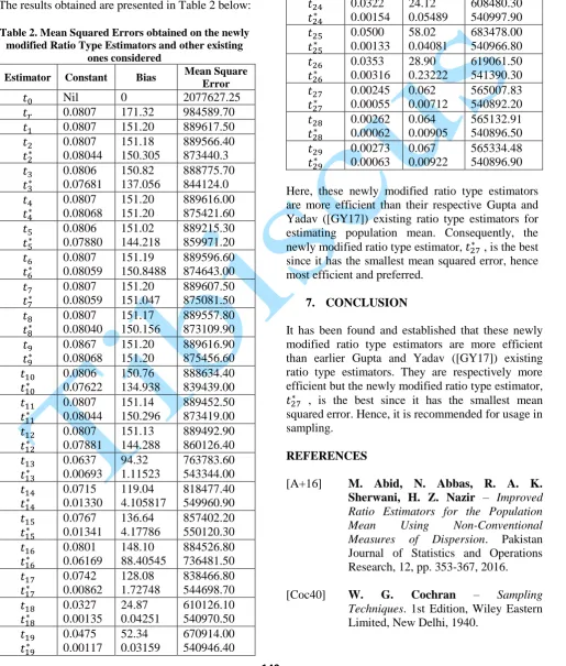
The results obtained are presented in Table 2 below:
Table 2. Mean Squared Errors obtained on the newly modified Ratio Type Estimators and other existing
ones considered
Estimator Constant Bias Mean Square Error
𝑡0 Nil 0 2077627.25
𝑡𝑟 0.0807 171.32 984589.70
𝑡1 0.0807 151.20 889617.50
𝑡2
𝑡2∗
0.0807 0.08044
151.18 150.305
889566.40 873440.3
𝑡3
𝑡3∗
0.0806 0.07681
150.82 137.056
888775.70 844124.0
𝑡4
𝑡4∗
0.0807 0.08068
151.20 151.20
889616.00 875421.60
𝑡5
𝑡5∗
0.0806 0.07880
151.02 144.218
889215.30 859971.20
𝑡6
𝑡6∗
0.0807 0.08059
151.19 150.8488
889596.60 874643.00
𝑡7
𝑡7∗
0.0807 0.08059
151.20 151.047
889607.50 875081.50
𝑡8
𝑡8∗
0.0807 0.08040
151.17 150.156
889557.80 873109.90
𝑡9
𝑡9∗
0.0867 0.08068
151.20 151.20
889616.90 875456.60
𝑡10
𝑡10∗
0.0806 0.07622
150.76 134.938
888634.40 839439.00
𝑡11
𝑡11∗
0.0807 0.08044
151.14 150.296
889452.50 873419.00
𝑡12
𝑡12∗
0.0807 0.07881
151.13 144.288
889492.90 860126.40
𝑡13
𝑡13∗
0.0637 0.00693
94.32 1.11523
763783.60 543344.00
𝑡14
𝑡14∗
0.0715 0.01330
119.04 4.105817
818477.40 549960.90
𝑡15
𝑡15∗
0.0767 0.01341
136.64 4.17786
857402.20 550120.30
𝑡16
𝑡16∗
0.0801 0.06169
148.10 88.40545
884526.80 736481.50
𝑡17
𝑡17∗
0.0742 0.00862
128.08 1.72748
838466.80 544698.70
𝑡18
𝑡18∗
0.0327 0.00135
24.87 0.04251
610126.10 540970.50
𝑡19
𝑡19∗
0.0475 0.00117
52.34 0.03159
670914.00 540946.40
Estimator Constant Bias Mean Square Error
𝑡20
𝑡20∗
0.0297 0.00279
20.59 0.18075
600579.70 541276.40
𝑡21
𝑡21∗
0.0320 0.00152
23.85 0.05388
607875.10 540995.7
𝑡22
𝑡22∗
0.0498 0.00131
57.60 0.04006
682552.70 540965.10
𝑡23
𝑡23∗
0.0351 0.00313
28.59 0.22803
618381.50 541381.00
𝑡24
𝑡24∗
0.0322 0.00154
24.12 0.05489
608480.30 540997.90
𝑡25
𝑡25∗
0.0500 0.00133
58.02 0.04081
683478.00 540966.80
𝑡26
𝑡26∗
0.0353 0.00316
28.90 0.23222
619061.50 541390.30
𝑡27
𝑡27∗
0.00245 0.00055
0.062 0.00712
565007.83 540892.20
𝑡28
𝑡28∗
0.00262 0.00062
0.064 0.00905
565132.91 540896.50
𝑡29
𝑡29∗
0.00273 0.00063
0.067 0.00922
565334.48 540896.90
Here, these newly modified ratio type estimators are more efficient than their respective Gupta and Yadav ([GY17]) existing ratio type estimators for estimating population mean. Consequently, the newly modified ratio type estimator, 𝑡27∗ , is the best since it has the smallest mean squared error, hence most efficient and preferred.
7. CONCLUSION
It has been found and established that these newly modified ratio type estimators are more efficient than earlier Gupta and Yadav ([GY17]) existing ratio type estimators. They are respectively more efficient but the newly modified ratio type estimator,
𝑡27∗ , is the best since it has the smallest mean squared error. Hence, it is recommended for usage in sampling.
REFERENCES
[A+16] M. Abid, N. Abbas, R. A. K. Sherwani, H. Z. Nazir – Improved Ratio Estimators for the Population
Mean Using Non-Conventional
Measures of Dispersion. Pakistan Journal of Statistics and Operations Research, 12, pp. 353-367, 2016.
[Coc77] W. G. Cochran – Sampling Techniques. 3rd Edition, New York: John and Sons, New Delhi, 1977.
[GY17] R. K. Gupta, S. K. Yadav. – New Efficient Estimators of Population Mean Using Non-Traditional Measures of Dispersion. Open Journal of Statistics 7, pp. 394-404, 2017.
[JMM13] M. I. Jeelani, S. Maqbool, S. A. Mir –
Modified Ratio Estimators of
Population Mean Using Linear
Combination of Coefficient of Skewness and Quartile Deviation. International Journal of Modern Mathematical Sciences, 6, pp. 174-183, 2013.
[KC04] C. Kadilar, H. Cingi – Ratio
Estimators in Simple Random
Sampling. Applied Mathematics and Computation, 151, pp. 893-902, 2004.
[KC06] C. Kadilar, H. Cingi - An
Improvement in Estimating the
Population Mean by Using the
Correlation Coefficient. Hacettepe Journal of Mathematics and Statistics, 35, pp. 103-109, 2006.
[SJ12] J. Subramani, G. Kumarapandiyan –
Estimation of Population Mean Using Co-Efficient of Variation and Median of an Auxiliary Variable. International Journal of Probability and Statistics, 1, pp. 111-118, 2012.