__________
* Corresponding author
E-mail addresses:[email protected](M.Esmaeilzade);[email protected](J.Amini) DOI: 10.22059/eoge.2019.248253.1018
1
Evaluation of a 2-D transformation model for georeferencing of Synthetic
Aperture RADAR imagery
Majid Esmaeilzadeh, Jalal Amini*
School of Surveying and Geospatial Engineering, College of Engineering, University of Tehran, Tehran, Iran
Article history:
Received: 2 October 2018, Received in revised form: 1 February 2019, Accepted: 12 February 2019 ABSTRACT
The Synthetic Aperture Radar (SAR) geometry imaging includes geometric distortions, which cause errors. To compensate the geometric distortions, the information about sensor position, imaging geometry, and target altitude from ellipsoid should be available. In this paper, a method for geometric calibration of SAR images is proposed. The method uses Range-Doppler (RD) equations. In this method, the georeferencing is carried out using the Digital Elevation Model (DEM) and also exact ephemeris data of the sensor. First, the digital elevation model is transferred to the range and azimuth directions. Then, the original image is registered to the transferred DEM from the previous step with transformation equations: conformal, affine, and projective. The advantage of the method described in this article is the elimination of required control points and rotational parameters of the sensor. Since the ground range resolution of used images is about 30m, in best stance, the geocoded images using the method described in this paper have an accuracy of about 20m (subpixel) in planimetry and of about 33m in altimetry.
S KEYWORDS
Range-Doppler Digital Elevation Model Transformation
Georeferencing Topographic errors
1. Introduction
Natural disasters such as floods, earthquakes, landslides, and adverse weather conditions are the greatest threats to the life of the human being. It is difficult to detect and manage the changes caused by these phenomena. Microwave active sensors are independent of the atmospheric condition and climate changes. Therefore, they are useful tools to overcome the climatic condition, but they need accurate information and correct data (Curlander & McDonough, 1991). In the SAR imagery, qualitative analysis of SAR images is employed to extract specific information for a variety of applications. In fact, in high altitude areas and rough surfaces, the incidence angle deflects from geoid and the accuracy of imaging geometry as a function of height that is
dependent on the geoid model decreases. Therefore, obtaining the correct information from image geometry is important (Chooet al.,2012).Inthe beginning, the Rational Function Models (RFM) (Grodecki et al., 2004) are used widely for geometric calibration of optical imagesand then, the RFMisused for geometric calibration oftheSAR data. The advantage oftheRFM model versustheRange-Doppler (RD)model is thattheRFM model is faster intheconversion of two dimensional(2D) image space into three dimensional (3D) object space, without significantly reducing the accuracy of the calculations (Eftekhari et al., 2013). The major problem is that3DfullyformofRFM models need at least 39 Ground Control Points (GCP) (depending on the degree of the used polynomial and 39 GCP is for the
2 maximum degree) in image scene to find Rational
Polynomial Coefficients (RPC)(Zhang et al., 2011
)
. Another method was based on SAR image simulation using DEM and registering the original image to the simulated image to compensate these errors. Then, the RPC model was used, but still, the availability of GCPs was problematic and needed surveying. (Zhang et al., 2012)
.The RD model was used to develop a mathematical model to locate the SAR image pixels, but this method was unable to eliminate foreshortening and layovers because it does not use other information sources such as GCP (Zhou et al., 2012)
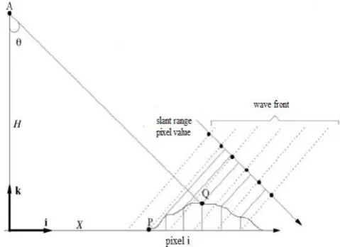
. As in the reviewed methods, the SAR georeferencing need GCPs. Nevertheless, the method proposed in this article does not use any ground control points, and it instead uses DEM for SAR image georeferencing. In side-looking radars, the angle of incidence (η), varies across the swath and the ground distance represented by each sample (pixel) is not uniform. As a result, the features in the near range appear compressed compared to the far range (Figure 1). The slant range spacing and the ground range spacing can be related by sin(η) only for smooth surfaces (Oliver & Quegan, 2004)
. As the local terrain deviates from a smooth surface, additional geometric distortion occurs in the SAR image relative to the actual ground dimension. This effect, illustrated in figure 2-a, is termed foreshortening when the slope of the local terrain 𝛼, is less than the incidence angle η Similarly, a layovercondition exists for a steep terrain where α≥η. For ground areas sloped toward the radar (α+), the effective incidence angle becomes smaller, thus increasing the cross-track pixel spacing. Ground areas sloped away from the radar (α-) have effectively a larger localincidence angle thus decreasing the range pixel size.In the relatively high relief areas, as shown in figure2-b, a layover condition may exist such that the top of a mountain is at a nearer slant range than the base. In this case, the image of the mountain will be severely distorted, with the peak appearing in the image at a nearer range position than the base.
The general workflow of the proposed method for geometric calibration of SAR images based ontheRD model is illustrated in figure3. According to the workflow, after reading Single Look Complex (SLC) raw images, the amplitude image is created. On the other hand, the DEM is transferred to a Range-Azimuth coordinate system. Then, depending on the presence or absence of Doppler frequency, the position oftheoriginal imageon the transferred DEM is determined. By registering the original image to the transferred DEM, the radar image is georeferenced,and the topography errors are removed.
The rest of this paper presents the mathematical
formulations. Experimental results showthetest results and their analysis.Finally, section 4 presents the discussions and conclusions.
3 Figure 3. The workflow of the proposed method for SAR georeferencing.
2. Materials and Methods
According to the proposed method in Figure 3, the digital elevation model is firstly transferred to the slant range direction, so that all points of the DEM, in addition to the geographic coordinates, also have coordinates in range and azimuth direction (Figure 4). Then, the location of pixels in the original image is found on the transferred DEM, and it is coregistered to the transferred DEM that is in range and azimuth direction to the original SAR image which has errors by using two-dimensional transformation equations. The DEM is free of topographic errors, and by transferring this model to the range and azimuth direction, the SAR image will be free of errors. Finally, by transferring the original SAR image and its radiometric information to the transferred DEM, the output is a georeferenced SAR image in the geodetic coordinate system whose topographic errors is eliminated.
In order to transfer the DEM into Range-Azimuth directions, pre-processing is necessary. All DEM points are in the geodetic coordinate system, but sensor positions are in an Earth Centered – Earth Fixed (ECEF) coordinate system. For this purpose, all DEM points should be transferred to the ECEF coordinate system to have the same coordinate system for later calculations. The equations in (You, 2000) are used to convert the coordinate from geodetic (φ, λ, h) to ECEF (X, Y, Z).
Figure 4. Transferring DEM to the slant range direction After coordinate conversion, the main goal is transferring the DEM to the Range-Azimuth coordinate system. The Range-Doppler equation is used for this purpose. Eqs (1) and (2) represent Range-Doppler models, respectively (Soumekh, 1999).
s t
R R R
(1) 2
( ).( )
DC s t s t
f V V R R
R
4 Where R is the slant range between sensor and target, Rt is
the target position vector, Rs = H + Ren is the sensor position vector, fDC is the Doppler centroid frequency, λ is the wavelength and Vs ,Vt are the sensor and target speed vectors, respectively (Figure 5).
Figure 5. The relationship between look angle, incidence angle, and a smooth spherical geoid model.
In order to simulate each pixel of the DEM in the range and azimuth direction, a distance and a time should be calculated to find a position in the range and azimuth direction, respectively. All coordinates (DEM and satellite orbit position) are in the ECEF coordinate system. The distance of each pixel in the DEM to all points of the satellite orbit position is calculated by Eq (8).
2 2 2
( DEM orb) ( DEM orb) ( DEM orb)
d X X Y Y Z Z (3)
Where (XDEM, YDEM, ZDEM) and (Xorb, Yorb, Zorb) are ECEF coordinates of the DEM and satellite orbit, respectively.
The minimum distance between the DEM and the satellite orbit (minimum value of all calculated d) is named (Rrng) and the corresponding time orbit that the satellite has a minimum distance is named (tm). This process is conducted for all DEM points, so each pixel of the DEM has a minimum distance and a corresponding time. Then, if the Doppler frequency is zero, the coordinates in the Range-Azimuth system are calculated using Eqs (4) and (5).
1 [2 (s rng min rng) / ]*
range f R R c x (4)
1 [ *(m 1)]*
azimuth PRF t t y
(5) Where minRrng is the minimum range, t1 is the beginning time of imagery, PRF is pulse repetition frequency, fs is the range sampling rate, c is the light speed, and Δx and Δy are pixel spacing in range and azimuth direction. If the Doppler frequency is not zero, corrections should be applied to the
range and azimuth direction. The corrected range and azimuth are expressed by Eqs (6) and (7). Fd is the satellite Doppler frequency.
2 2 2
2 1 ( d rng s/ 4 s )
range range
F R f cV(6)
2
2 1 ( d rng / 2 s)
azimuth azimuth PRF F R
V(7) The above equations transfer the DEM to the Range-Azimuth coordinate system. The produced image is a DEM that has a coordinate in the range and azimuth system and also longitude, latitude, and height coordinates from the ellipsoid.
Thus, for each point in the DEM, the geodetic coordinates are converted to ECEF coordinates. Then a distance and a corresponding time that belong to the specific point of the DEM are calculated, and finally, the position of all DEM point is determined in the Range-Azimuth coordinate system. The procedure of geolocation can be sketched as the following transformation chain:
( , , ) h ( , , )X Y Z (tm rng, )(azimuth range, )
Finally, by registering the original image that has the geometric errors into the transferred DEM, the output image is georeferenced. All errors are eliminated on the georeferenced image.
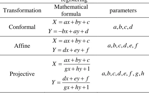
Three methods are used for registering the original image to the transferred DEM for solving the RD: Conformal, Affine, and Projective. Their mathematical formula and parameters are expressed in table 1.
Table 1. Transformation equation used for SAR image registering
Transformation Mathematical
formula parameters
Conformal X ax by c
Y bx ayd a b c d, , ,
Affine X ax by c
Ydx ey f a b c d e f, , , , ,
Projective 1
ax by c X
gx hy
1
dx ey f Y
gx hy
, , , , , , ,
a b c d e f g h
Where (X,Y) are the coordinates in the transferred DEM, and (x,y) are the coordinates in the original SAR image. In order to determine the {a,b,c,d,e,f,g,h} coefficients using the projective transformation, at least four known points are needed in both images. Affine and Conformal transformations need at least three and two known points. Four corners of both images can be used as known points.
5 lower spatial resolution than most satellite SAR data. Thus,
each DEM resolution cell corresponds to a clique of the SAR images that may contain many pixels. Therefore, the SAR images should be multi-looked to reduce speckle noise and convert rectangular pixel to square pixel. The multi-look factors are determined by a comparison between the DEM resolution and the SAR image sampling spacing in the azimuth and range, as expressed in the following Eqs:
sin / 2 0.5
A DEM r
N
(8)
/ sin 0.5
R A r a
N N
(9) Where NA and NR are the multi-look factors in azimuth and range pixel dimensions, respectively. σDEM is the DEM resolution, σa and σr respectively indicate the azimuth line spacing, and the range pixel spacing of the SAR image, is the SAR look angle. ⌊ ⌋ is the operator of the integer truncation (Zhang et al., 2011
)
.3 Experimental results
Four tests are carried out in this study for different purposes. The first test is to find the best transformation equation among the three types for registering images. The other test is to compare the georeferenced SAR images generated from three DEMs to demonstrate the effectiveness of the DEM spatial resolution on the accuracy of georeferencing SAR images. The third purpose is to study the effect of the size of datasets and data subsets on image accuracy. The last experiment is comparing the result of the proposed model with that of the RF model.
3.1. Datasets
In this study, two SAR datasets are tested with RD
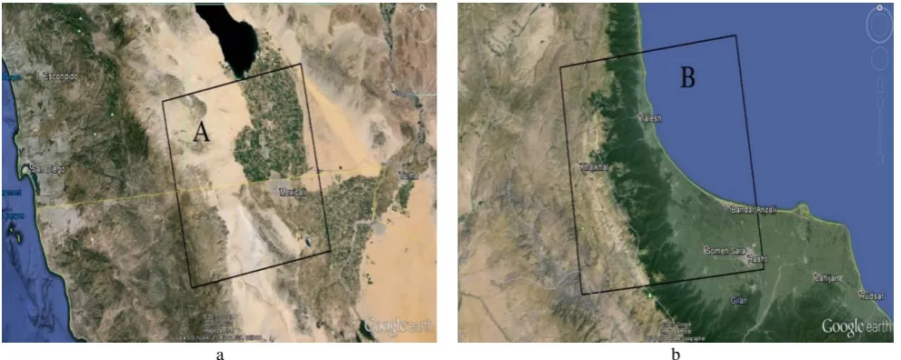
modeling. An ALOS PALSAR spaceborne SAR sensor acquires these datasets. Test areas covered by these datasets range from even plains to mountainous areas. The first dataset is located on the border between the United States and Mexico, and the second one is in Iran. Figure 5 shows the vicinity of the datasets captured from Google Earth. The rectangles in figure 6 show the coverage of these datasets. The urban area of El Centro and Mexicali near the Salton Sea together, as well as the surrounding mountain and farmlands, are selected as the first dataset. The second dataset is the mountainous and forest area near the Caspian Sea, Rasht, and Bandar Anzali in Iran. The necessary information about these test datasets is summarized in table 2. For convenience, we indexed these datasets with letters A and B, also shown in figure 6. The nominal ground range resolution of ALOS
PALSAR is about 30 meter while in azimuth the resolution is about 6 meters.
Three types of global DEM datasets are used as the referenced DEM for SAR image georeferencing particularly, including the ASTER GDEM V2, the SRTM DEM, and the ACE2 GDEM. The spatial resolutions are 1, 1, and 9 arcseconds for dataset A, and 1, 3, and 9 arc seconds for dataset B, respectively, i.e., approximately 30, 90, and 270 meters. The SRTM DEM has 1-arcsecond resolution just over the United States territory, and 3-arcsecond resolution in other areas. The Altimeter Corrected Elevation, 2nd edition (ACE2) GDEM was created by the De Montfort University of United Kingdom by merging the SRTM datasets with other elevation information from various data sources such as Satellite Radar Altimetry (Berry et al., 2010).
3.2. Pre-processing
ALOS PALSAR datasets are in level 1.0 in an SLC format. PALSAR sensor images are usually at processing level 1.0, 1.1, and 1.5. Level 1.0 images result from the processing of raw data in level 0, in which each pixel is expressed as a complex number I+jQ. I and Q are real and imaginary parts of the SLC images in level 1.1. Level 1.1 images are non-georeferenced amplitude images. The magnitude (A) of each pixel is obtained by Eq (10).
2 2
A I Q
(10)
Level 1.5 images are georeferenced amplitude images.
This study aims to apply the processes to transfer images from level 1.0 to level 1.5.
With ALOS images inlevel 1.0,there are two files,*.PRM
and*.0__A extensions. The PRM file contains information about sensor parameters such as earth radius, earth equatorial and polar radius, Doppler frequency, pulse duration, wavelength, range sampling rate,and image dimensions.The 0__A file, whichis calledtheleader file, contains the time of imaging with an accuracy ofamillisecondas well as precise ephemeris data such as position and velocity state vectors of the satellite. Both files are necessary for SAR georeferencing.
Using Eq (16), the single-look and multi-look amplitude
images are showninfigure7.In order toreduce the speckle noise,amulti-lookingprocess wasperformed on single-look images.NAand NRare selected in such a way thatthe spatial resolution of the image intherange and azimuth dimensions are approximately equal. The obtained multi-look images have 30 meters spatial resolution in both dimensions. Table 2. Basic information on the test datasets.
SAR sensor Data
index Observed area
Acquisition date
Imaging mode
Processing level
Image size (line by
pixel)
Elevation range (m)
ALOS PALSAR A El Centro, Mexico
2009.09.11 FBD SLC 27648 ×
11304
(-115 , 1800)
ALOS PALSAR B Rasht, Iran 2008.07.19 FBD SLC 27648 × 5652
6
a b
Figure 6. Geographic location and coverage of test datasets. (a) El Centro, Mexico, (b) Rasht, Iran
a b
c d
7
3.3. Results and discussion
3.3.1. Efficacy assessment of transformation equations on the RD model
In the first test, three methods are evaluated in terms of overall planimetry and altimetry accuracy for registering the original image to the transferred DEM for solving the RD. For georeferencing images, the ASTER GDEM is selected as the reference DEM.
The control points are required for georeferencing the original SAR image into the transferred DEM and using 2-D transformation equations. For this purpose, 20 control points are identified in dataset A and B by using Google Earth. Application of a different number of control points to solve transformation equations results in different values of degrees of freedom. Figure 8 shows the georeferenced SAR images in which are used projective transformation and a value of 30 for the degrees of freedom.
For accuracy evaluation, 25 checkpoints are manually selected in two images to determine the planimetry and altimetry accuracy. They are distributed within the scene and carefully located at stable and flat ground shown as yellow spots in figure 8. Points that are chosen in the mountainous area are shown as red spots in figure 8. Each point has two sets of coordinates: coordinates obtained using the method presented in this study and point coordinate from Google Earth that is considered as a reference. For accuracy determination, the planimetry and altimetry Root Mean Square Error (RMSE) of each point are calculated by Eqs (11) and (12):
2 2
1 1
1
( ) [ ( ) ( )
n n
i i i i
i i
RMSE planimetry X x Y y
n
(11)
2
1
1
( ) [ ( )
n
i i i
RMSE altimetry H h n
(12)
where(X,Y, H)are the longitude, thelatitude, andthe
height coordinates of the georeferenced image, and respectively(x, y, h)are the same items from Google Earth.
To demonstrate the effectiveness of the transformation
equations andthedegrees of freedom on georeferencing, we performed all three types of transformations in 16 different levels of the degrees of freedom for both datasets. The experimental results are given infigures9and10.
The location errors significantly reduced,especiallyfor the
conformal transformation equation. Furthermore, with the RD model and usingtheprojective transformation equation witha value of30 for the degrees of freedom, the RMSE valuesof location errors ofthegeoreferenced SAR images in planimetry are 20.11m for dataset A and 19.94 for dataset B. Both of these values are less than 30meters, i.e.,the nominal ground range resolution of ALOS PALSAR images. In other words, a geolocation accuracy better than the one-pixel accuracy ofthe SAR images is obtained. This table shows that for degrees of freedom 24 and more, planimetry RMSEs areaconvergentand increasing degreeof freedom is futile. Figures9and10confirmed thatthebest equation for SAR image georeferencing is the projective transformation equation.
a b
8 3.3.2. Evaluation of different DEMs for georeferencing on
the RD model
In this test, the impact of the DEM resolution on the RD solution is evaluated with datasets A and B. The projective method is used for registering images. The variation of overall planimetry and altimetry RMSE of datasets A and B, along with the DEM types, are presented in Fig. 11 and 12.
It can be seen that for both datasets, the overall RMSE increased by increasing the DEM pixel size. The above mentioned experimental results show that in dataset A, SRTM DEM has less accuracy compared to ASTER GDEM although both of ASTER GDEM and SRTM DEM have 1 arcsecond DEM resolution and their accuracy is acceptable. It shows that in an equal condition, ASTER GDEM is more accurate than SRTM DEM.
Another conclusion that can be obtained by this experiment is that by comparing the equal condition of datasets A and B (in ASTER GDEM or ACE2 GDEM), dataset B is more accurate than dataset A. This accuracy is due to images size. Pixel numbers on range dimension in dataset B is exactly half of the pixel numbers in the same direction in dataset A.
We can easily conclude that the higher the resolution of the DEM, the better the accuracy of the georeferenced SAR image. In this case study, the accuracy of the georeferenced image from ASTER GDEM and SRTM are acceptable. Figures 10 and 11 show that ASTER GDEM is more accurate than SRTM DEM. The georeferenced image that used ACE2 GDEM shows a bad accuracy and could not be used for georeferencing SAR images on the RD model.
Figure 11. The plot of overall planimetry RMSE versus DEM type and degree of freedom
Figure 12. The plot of overall planimetry RMSE versus DEM type and degree of freedom
1900 2900 3900 4900 5900 6900
0 5 1 0 1 5 2 0 2 5 3 0
O ve ral l p lan im et ry R M SE [m m ]
Degree of freedom
ASTER GDEM A SRTM DEM A ACE2 GDEM A
ASTER GDEM B SRTM DEM B ACE2 GDEM B
1900 2900 3900 4900 5900 6900
0 5 1 0 1 5 2 0 2 5 3 0
O ve ral l p lan im et ry R M SE [m m ]
Degree of freedom
ASTER GDEM A SRTM DEM A ACE2 GDEM A
ASTER GDEM B SRTM DEM B ACE2 GDEM B
Figure 9. Plot of overall planimetry RMSE versus degree of freedom and transformation equations
Figure 10. Plot of overall altimetry RMSE versus degree of freedom and transformation equations
1900 2400 2900 3400 3900 4400 4900
0 5 1 0 1 5 2 0 2 5 3 0
O ve ral l pl an im et ry R M SE [ m m ]
Degree of freedom
Conformal A Affine A Projective A
Conformal B Affine B Projective B
3200 3700 4200 4700 5200 5700
0 5 1 0 1 5 2 0 2 5 3 0
O ve ral l al ti m et ry R M SE [ m m ]
Degree of freedom
Conformal A Affine A Projective A
9 3.3.3. Computation time for SAR georeferencing with the
RD model
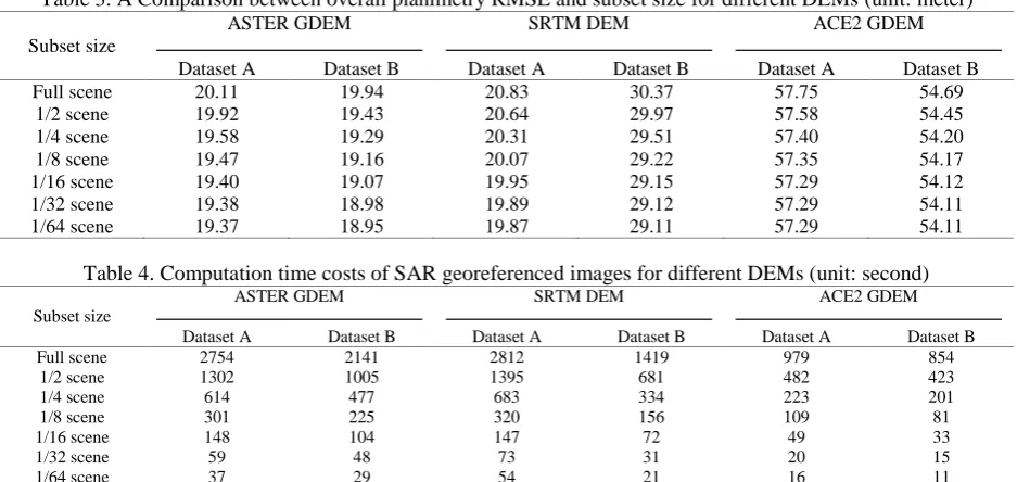
In this test, SAR georeferencing is evaluated in terms of computation time. Datasets A and B are taken as the test SAR image and three DEM datasets of different spatial resolution, including ASTER GDEM, SRTM DEM, and ACE2 GDEM, act as the reference DEMs. Since the Computation time may change with different image sizes, we made subsets of different sizes from the test SAR image. The selected subsets have seven levels from full scene to 1/64 of the scene. For each subset size, both of the datasets are employed with three references DEMs to georeference the subset of the SAR image. The overall planimetry RMSE and the computation time costs for all combinations are seized and represented in tables 3 and 4, respectively. All computations are carried out on a laptop equipped with an Intel CoreTMi7 Q740 CPU of frequency 1.73 GHz, 4GB DDR3 RAM and MS Windows 10, 64-bit version.
Table 5 shows that for all subsets and reference DEM type, the overall planimetry RMSE will decrease when the image size is reduced. For ACE2 GDEM, the variation of overall
RMSE along with different subset sizes is big enough to be considered almost constant in small image sizes. However, for the SRTM DEM and ASTER GDEM, such variations seem to be remarkable and can be evaluated by linear models. Table 6 and figure 13 show that for a fixed dataset when the image size decreases, the computation time reduces exponentially.
Figure 13. The plot of the RD model speedup for different DEM type and SAR image subset size
Table 3. A Comparison between overall planimetry RMSE and subset size for different DEMs (unit: meter) Subset size
ASTER GDEM SRTM DEM ACE2 GDEM
Dataset A Dataset B Dataset A Dataset B Dataset A Dataset B
Full scene 20.11 19.94 20.83 30.37 57.75 54.69
1/2 scene 19.92 19.43 20.64 29.97 57.58 54.45
1/4 scene 19.58 19.29 20.31 29.51 57.40 54.20
1/8 scene 19.47 19.16 20.07 29.22 57.35 54.17
1/16 scene 19.40 19.07 19.95 29.15 57.29 54.12
1/32 scene 19.38 18.98 19.89 29.12 57.29 54.11
1/64 scene 19.37 18.95 19.87 29.11 57.29 54.11
Table 4. Computation time costs of SAR georeferenced images for different DEMs (unit: second) Subset size
ASTER GDEM SRTM DEM ACE2 GDEM
Dataset A Dataset B Dataset A Dataset B Dataset A Dataset B
Full scene 2754 2141 2812 1419 979 854
1/2 scene 1302 1005 1395 681 482 423
1/4 scene 614 477 683 334 223 201
1/8 scene 301 225 320 156 109 81
1/16 scene 148 104 147 72 49 33
1/32 scene 59 48 73 31 20 15
1/64 scene 37 29 54 21 16 11
3.3.4. Comparing the result of SAR georeferencing with RD model and RF model
In the last experiment, the RD and RF models are applied to dataset A and B. The purpose of this test is to compare the accuracy of these models. The first test shows that the projective transformation equation is the best, so the projective equation is used for registering images. The second test demonstrates that the ASTER DEM has a better performance than other DEMs. As a result, the ASTER DEM is chosen as a reference DEM in this test. The result of applying the proposed RD model and fully RFM are presented in Fig. 14 and 15. The RPC of the rational function
model is obtained by 39 GCPs,which is chosen manually and carefully measured in Google Earth.The figures show that for bothdatasets, the overall planimetry and altimetry RMSE forthe RD model isa littlebetter thanthefullyRF model. By increasing the degree of freedom, the planimetry and altimetry RMSEvalues decrease. It is worth notingthat if one measures the GCP coordinates with GPS, the overall accuracy might be better for boththeapplied models. Some researchers proposed refined RF models which have excellentperformance and accuracy. We usedasimple RF model with amaximum degree of the polynomial without any refinement for comparing withtheproposed RD model.
0 500 1000 1500 2000 2500 3000
F u l l s c e n e
1 / 2 s c e n e
1 / 4 s c e n e
1 / 8 s c e n e
1 / 1 6 s c e n e
1 / 3 2 s c e n e
1 / 6 4 s c e n e
C
o
m
pu
tat
io
n
ti
m
e [
s]
Data size
ASTER GDEM A SRTM DEM A ACE2 GDEM A
01 Figure 14. The plot of overall planimetry RMSE versus the
type of used model (RD and RF) and degree of freedom
Figure 15. The plot of overall altimetry RMSE versus the type of used model (RD and RF) and degree of freedom 4. Conclusion
Geometric calibration and georeferencing are the most images. Geometric SAR raw
of processes important
distortions are caused by platform instabilities, error in determining the relative height and displacements due to topography. In order to georeference a SAR image, an independent source of information was required, such as imaging from another angle, topographic map, or DEM.
For SAR image georeferencing and removing topographic errors, the DEM is considered as an independent source of information. An approach based on transferred DEM and registering between the original SAR image and the transferred DEM was developed to correct the topographic errors. The main advantage of the proposed method is that it does not require any GCPs. In order to evaluate the potency of the developed approach for the RD model, four tests were executed. In the first test, the efficacy of three types of transformation equations was evaluated on georeferencing of
selected with
ALOS PALSAR images checkpoints To.
evaluate the accuracy of the georeferenced images, we selected 25 checkpoints in different parts of the image. By comparing the obtained coordinates in the georeferenced image and reference points in Google Earth, the RMSE was calculated for these points. In the best situation, the planimetry accuracy was 20.11m for dataset A and 19.94m for dataset B, and the altimetry accuracy values were 33.28m for dataset A and 32.71m for dataset B. Since the ground resolution of multi-look image was 30 meters, the planimetry accuracy achieved in this research is acceptable. In the next two tests, the location errors of georeferenced ALOS PALSAR images with three types of DEMs were evaluated as reference DEM and subsets of images. In the last one, the accuracy of the RD and RF models is compared and shows that the proposed method has higher accuracy than the RF model. In addition, we studied the compatibility of three typical DEM datasets for SAR georeferencing in the RD model. The results represented that the best transferred DEM was obtained from ASTER GDEM.
References
Curlander, J. C., & McDonough, R. N. (1991). Synthetic aperture radar- Systems and signal processing(Book). New York: John Wiley & Sons, Inc, 1991.
Choo, L., Chan, Y. K., & Koo, V. C. (2012). Geometric correction on SAR imagery. In Progress in Electromagnetics Research Symposium Proceedings, KL, MALAYSIA.
Grodecki, J., Dial, G., & Lutes, J. (2004). Mathematical model for 3D feature extraction from multiple satellite images described by RPCs. In ASPRS Annual Conference Proceedings, Denver, Colorado.
Eftekhari, A., Saadatseresht, M., & Motagh, M. (2013). A study on rational function model generation for TerraSAR-X imagery.Sensors,13(9), 12030-12043. Zhang, L., He, X., Balz, T., Wei, X., & Liao, M. (2011).
Rational function modeling for spaceborne SAR datasets.ISPRS journal of Photogrammetry and Remote Sensing,66(1), 133-145.
Zhang, L., Balz, T., & Liao, M. (2012). Satellite SAR geocoding with refined RPC model. ISPRS journal of photogrammetry and remote sensing,69, 37-49.
Zhou, X., Zeng, Q., Jiao, J., Wang, Q., & Gao, S. (2012). Geometric calibration and geolocation of airborne SAR images. In 2012 IEEE International Geoscience and
Remote Sensing Symposium(pp. 4513-4516). IEEE.
Oliver, C., & Quegan, S. (2004). Understanding synthetic aperture radar images. SciTech Publishing.
You, R. J. (2000). Transformation of Cartesian to geodetic coordinates without iterations. Journal of Surveying Engineering,126(1), 1-7.
Soumekh, M. (1999). Synthetic aperture radar signal
processing (Vol. 7). New York: Wiley.
Berry, P. A. M., Smith, R. G., & Benveniste, J. (2010). ACE2: the new global digital elevation model. In Gravity, geoid and earth observation (pp. 231-237). Springer, Berlin, Heidelberg.
Curlander, J. C. (1982). Location of spaceborne SAR imagery. IEEE Transactions on Geoscience and Remote Sensing, (3), 359-364.
(2008). C.
J. Souyris, &
Massonnet, D., Imaging with
synthetic aperture radar. EPFL press.
1900 2100 2300 2500 2700 2900 3100 3300
0 2 4 6 8 10 12 14 16 18 20 22 24 26 28 30
O ve ral l pl an im et ry R M SE [ m m ]
Deegree of freedom
RD model A RF model A
RD model B RF model B
3200 3400 3600 3800 4000 4200 4400 4600
0 2 4 6 8 10 12 14 16 18 20 22 24 26 28 30
O ve ral l al ti m et ry R M SE [ m m ]
Deegree of freedom
RD model A RF model A
00 Shimada, M., Isoguchi, O., Tadono, T., & Isono, K. (2009).
PALSAR radiometric and geometric calibration. IEEE Transactions on Geoscience and Remote Sensing, 47(12), 3915-3932.
Yuan, X., & Lin, X. (2008). A method for solving rational
polynomial coefficients based on ridge
estimation. Geomatics and Information Science of Wuhan University, 33(11), 1130-1133.
Earth Observation Research and Application Center, Japan Aerospace Exploration Agency, ALOS data user handbook Revision C, (2008).
European Space Agency, information on ALOS PALSAR product for Aden users, (2007).