I.
Introduction
I
N recent years, the continuous development of electrical loads, especially due to industrial plants and human activities, results in increased number of new transmission lines, power plants, distribution networks and interconnection between different power systems. This effect leads to higher currents and power losses accompanied by voltage drop. Distribution system (DS) is an essential part of this power system problem as it connects loads to the transmission line at substations. About 70% of the power system losses are occurring at distribution system [1]. Therefore, the reduction of the losses in DS is the main concern nowadays. Hence, the world directed to use new generation sources of renewable energy resources (RERs) such as photovoltaic (PV), wind turbines and biomass energy, which are considered economically for supplying energy to electrical grids and suitable for power generation in remote areas [2], [3]. There are many potential benefits of DGs depending on their size and location. Normally, the real power loss and the voltage profile are the base objectives. Someother technical parameters may accompany this base objective such as reactive power requirement, reliability and efficiency of distribution network, emission, load-ability, voltage stability, DG capacity maximization, or economy oriented objectives [4]. There are different types of DG units, which can be classified based on whether they generate or absorb reactive power along with active power generation to (a) type A-DG units or P-type, which produces active power only such as PV (b) type B-DG units or Q-type, which produces reactive power only, like capacitor banks (c) type C-DG units or PQ+-type, which produces active and reactive power like synchronous generators (d) Type D-DG units or PQ--type which produces active power and consumes reactive power, like wind power induction generators.
The random placement of DGs and capacitors in DS can cause more voltage drop and higher power losses than losses without them [5], [6]. Therefore, determining the proper placement and capacity of DGs in DS becomes a crucial task for obtaining their maximum possible advantages. Several techniques have been proposed in recent years to determine the optimal locations and sizes of DGs in DS such as Ref. [7], which discussed the adaptive protection using neural networks for high penetration of DGs, but this technique takes very long training time. Ref. [8] made a very hard work to get the effective signals for optimal ratings of RERs as the objective function and
Genetic-Moth Swarm Algorithm for Optimal
Placement and Capacity of Renewable DG Sources in
Distribution Systems
Emad A. Mohamed
1,2*, Al-Attar Ali Mohamed
2, Yasunori Mitani
11
Department of Electrical Engineering, Kyushu Institute of Technology, 1-1 Sensui-cho, Tobata-ku,
Kitakyushu-shi, Fukuoka 804-8550 (Japan)
2
Department of Electrical Engineering, Aswan University, 81542 Aswan (Egypt)
Received 13 August 2019 | Accepted 19 November 2018 | Published 30 October 2019
Keywords
Radial Distribution System, Renewable Distributed Generation, Power Loss, Genetic-Moth Swarm Algorithm.Abstract
This paper presents a hybrid approach based on the Genetic Algorithm (GA) and Moth Swarm Algorithm (MSA), namely Genetic Moth Swarm Algorithm (GMSA), for determining the optimal location and sizing of renewable distributed generation (DG) sources on radial distribution networks (RDN). Minimizing the electrical power loss within the framework of system operation and under security constraints is the main objective of this study. In the proposed technique, the global search ability has been regulated by the incorporation of GA operations with adaptive mutation operator on the reconnaissance phase using genetic pathfinder moths. In addition, the selection of artificial light sources has been expanded over the swarm. The representation of individuals within the three phases of MSA has been modified in terms of quality and ratio. Elite individuals have been used to play different roles in order to reduce the design space and thus increase the exploitation ability. The developed GMSA has been applied on different scales of standard RDN of the (33 and 69-bus) power systems. Firstly, the most adequate buses for installing DGs are suggested using Voltage Stability Index (VSI). Then the proposed GMSA is applied to reduce real power generation, power loss, and total system cost, in addition, to improve the minimum bus voltage and the annual net saving by selecting the DGs size and their locations. Furthermore, GMSA is compared with other literature methods under several power system constraints and conditions, in single and multi-objective optimization space. The computational results prove the effectiveness and superiority of the GMSA with respect to power loss reduction and voltage profile enhancement using a minimum size of renewable DG units.
* Corresponding author.
E-mail address: [email protected]
constraints are designed using fuzzy sets. In Ref. [9] authors discussed the achievement of the trade-off between the reliability improvement and DG capacity by examining the load shedding.
Recently, numerous optimization algorithms handled the problem of DGs locations and sizing in DS. Artificial bee colony (ABC) [10], Genetic Algorithm (GA) [11], cuckoo search algorithm (CSA) [12], mixed integer nonlinear programming (MINLP) [13], Differential Evolution (DE) [14], flower pollination algorithm (FPA) [15]. Although these heuristic algorithms have been implemented simply and free derivative, they need numerous iterations to guarantee that the solution is converged. Hence, these techniques are computationally intensive. Furthermore, some studies used hybrid algorithms with analytical to combine their features and eliminate the shortage like, simulated annealing uses Loss Sensitivity Factor (LSF) in [16], PSO uses sensitivity analysis in [17], and hybrid PSO in [18]. There is another type of hybridization, which is combining metaheuristic algorithms together such as, genetic algorithm (GA) with imperialist competitive algorithm [19], ant colony optimization with artificial bee colony (HACO) [20], hybrid grey wolf optimizer (HGWO) [21], backtracking search optimization algorithm (BSOA) [22], and in [23], which used particle ant bee colony with harmony search (PABC). Other studies used the analytical approach such as in [24], which uses efficient analytical with optimal power flow (EA-OPF), an improved analytical (IA) method in [25] and machine learning method in [26]. In addition to Naresh, who used an analytical expression for optimum location for DG [27]. Most of previous techniques use a simple single objective function for minimizing the power losses except [19], [21], [23] that use a multi-objective functions to reduce real losses and improve voltage stability. Further, only few methods deal with the renewable DGs like in [20], [22], ant lion optimization (ALO) algorithm in Ref. [28], and backtracking search (BSA) algorithm in Ref. [29]. The above mentioned algorithms seem to be efficient. However they may not guarantee reaching the optimal value and face difficulty in escaping from the local minimum as the power losses face nonlinear equality constraints. This makes the problem non-convex.
A new hybrid GMSA is developed based on the incorporation of GA operations with adaptive mutation operator on the reconnaissance phase using genetic pathfinder moths and the expanding of artificial light sources over the swarm. The GMSA has some advantages over the other swarm algorithms such as (i) its simplicity and flexibility as it can be applied to different problems without changing the main algorithm structure. (ii) ability on avoiding the trap in local minima. (iii) achieving fast convergence characteristics [30]. Ref. [30] determined the optimal sizes and locations of DGs without considering the different types of DGs. In this paper, three types of DG units including PV, WTG, and capacitor bank based DGs are embedded in distribution system optimally for minimizing the power losses. A sensitivity analysis based-Voltage Stability Index (VSI) has been performed to determine the most candidate locations for inclusion the compensation devices in DS to reduce the search space of optimization techniques and simulation time. Then, the hybrid approach based on the genetic algorithm (GA) and moth swarm algorithm (MSA) [31], is presented to determine the optimal renewable DG capacity and locations in the DS to minimize the system power losses, and maintain the voltage profile for various electrical distribution systems. It is tested on standard distribution systems i.e., (33 and 69 -bus). In addition, the obtained results from the proposed approach are compared with those obtained from other algorithms to confirm its superiority. The article is organized as follows; section II provides the objective function formulation. GMSA algorithm is represented in section III. In section IV, the implementing of GMSA code for solving the DGs allocation problem has been presented. Section V shows the numerical results of the proposed technique applied on multiple standard systems. The last section concludes the results and advantages of the proposed method.
II.
Problem Formulation
A. Load Flow Calculation
Radial distribution networks (RDN) creates some negative conditions such as radial meshed networks, unbalanced operation, high R/X ratios and distributed generation. Due to these problems, the Newton Raphson, Gauss Siedel and other conventional load flow algorithms are not effective to solve the load flow calculation of the distribution systems [32]. Therefore, the modern algorithm called backward/forward sweep [32] is used in this work to analyze the power flow in the tested IEEE distribution systems. Fig. 1 shows a single line diagram of RDN. The active power flow (Pk+1) and reactive power flow (Qk+1) in RDN including DG unit at bus (k+1) are calculated by (1) and (2):
(1)
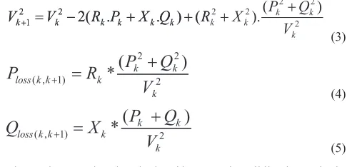
(2) where, k is the sending end and k+1 is the receiving end. Voltages of a transmission line and real power losses in the line can be calculated from (3), (4), and (5) respectively:
(3)
(4)
(5) The total system loss is calculated by summing all line losses in the system as shown in (6):
(6)
Pk, Qk Pk+1, Qk+1
Rk+ JX k
PLk+ JQ Lk PL(k+1)+ JQL(k+1)
Vk V
k+1
Fig. 1. Simple radial distribution system.
The system security level is important and can be determined using the voltage stability index as follows:
(7) VSI should be high in order to improve the voltage profile and this can be achieved by minimizing the voltage deviations (VD) as follows:
where, n is the number of buses and Vref is the reference voltage, which commonly is 1 p.u.
B. Objective Functions
The main aim of the optimal DG placement problem is to minimize the voltage deviation, reduce the real power losses and improve the system voltage stability. There is a contrasting relation between these objectives, as clearly identified and numerically obtained by [33]. Hence, the multi-objective functions have been performed by using the following mathematical statements:
(9)
(10)
(11) where, nl is number of branches in RDN and nb is number of buses.
The weighted sum method is used to evaluate the effectiveness of the proposed approach for optimal placement and sizing of DG units. The concept Pareto strategy is not appropriate for such purpose, where the challenge in multi-objective optimization based on Pareto strategy is to find the Pareto optimal point that meets the decision maker’s given preferences. From the perspective of mathematical optimization, the weighted sum method allows the multi-objective to be cast as a single-objective mathematical optimization problem resulting in only one solution, in addition to its lower computational cost (CPU-time). These advantages are more proper for real world problems. Therefore, the generalized objective function based on weighted sum method can be formulated as follows:
(12) where, w1, w2, and w3 are weighting factors. The value of any
weighting factor is selected based on the relative importance on the related objective function with others objective functions. The sum of the absolute values of the weight factors in (12) subjected to all impacts should equal one:
(13)
C. Constraint Conditions
The multi-objective functions are subjected to the following constraints:
1. Active and Reactive Power Balance
The active and reactive power flow constraints, which represent the equality constraints could be established for maintaining the balance between generation and consumption.
(14)
(15)
2. Voltage Constraints
The buses voltages are the inequality constraints. The bus voltage magnitude of each bus must be maintained within the following range:
(16) where Vmax and Vmin are the maximum and minimum values of bus (k) voltages. The lower and upper values are taken as 0.9 and 1.05 Pu, respectively.
3. DG Capacity Limits
The constraints of DG capacities are as follows:
(17)
(18)
(19)
(20)
(21) where, and are the minimum and maximum real outputs of the DG source. and are the minimum and maximum power factor of the DG source.
The input control vector xc is composed of independent adjustable variables for each DG units. Each DG has three input control variables: location (L), power factor (PF) and injecting active power (PDG). Multiple DG units can be installed in a system as follows:
=
,
, … ,
,
,
,
,
,
,
, … ,
(22) In this paper, in the case of capacitor banks, the PF is zero and for PV units, the PF is considered to be unity thus the DG unit only delivers active power. While, in the case of wind, the DG unit delivers active and reactive power.
D. Equality and Inequality Constraints Treatment
Power-flow equations, equality constraints (14) and (15), can be satisfied during the process of power-flow calculation. In the encoding period, the inequality constraints (16)–(21) can be satisfied through adding penalty function into the objective function in such a way that it penalizes any violation of the constraints. Consequently, the constrained optimization problem is then converted into an unconstrained form.
III. Overview of GMSA
A. Genetic Algorithms
have been applied successfully to solve a large number of problems in different real-world fields by simulating the natural evolution systems. The recombination operation produces offspring that carry a combination of genetic material information from each parent where crossover operations are applied to exchange the chromosomes. The natural selection determines the evolution where the fittest survives with higher probability. Therefore, a suitable selection strategy is then used to determine the solutions that survives to the next generation based on their fitness values. The mutation operation is the main genetic operator that can achieve some diversity in the population.
The steps of the MSA technique are discussed below.
B. Moth Swarm Algorithm
The moth swarm algorithm has been presented in 2017 by Al-Attar et al. [30]. It is inspired by the orientation of moths towards moonlight. The available solution of an optimization problem using MSA is performed by the light source position, and its fitness is the luminescence intensity of the light source. Furthermore, the proposed method consists of three main groups, the first one is called pathfinders which are considered a small group of moths over the available space of the optimization. The main target of this group is to guide the locomotion of the main swarm by discriminating the best positions as light sources. Prospectors group is the second one which has a tendency to expatiate in a non-uniform spiral path within the section of the light sources determined by the pathfinders. The last one is the onlookers, this group of moths move directly to the global solution which has been acquired by the prospectors.
C. Genetic Moth Swarm Algorithm (GMSA)
The proposed hybrid based algorithm aims to integrate advantages of the well-known GA in terms of sharing information and global search ability to find the optimal value of a given function using the following steps:
1. Initialization
Initially, the positions of moths are randomly created for dimensional (d) and population number (n) as seen in (23).
(23) where, xjmax and x
jmin are the upper and lower limits, respectively. Afterwards, the type of each moth is selected based on the determined fitness. Consequently, the worst moths are selected as pathfinders that are modified to act genetically in the following reconnaissance phase. In the next two phases, the best individuals of the swarm are regarded as prospectors and onlookers, respectively, according to their fitness. In addition, each moth in the modified algorithm has its own light source which is available to share with others in the swarm.
2. Genetic Reconnaissance Phase
The moths may be concentrated in the regions which seem to provide good performance. Therefore, the swarm quality for reconnaissance may be decreased during processing the optimization and this process may lead to a stagnation case. To avoid the early convergence and enhance the solution diversity, a part of the swarm is compelled to determine the less congested area. The pathfinder moths that perform this role are manipulated to evolve by the genetic operators, with the size of (np=floor (n/2)) selected from the worst-performing individuals in the swarm. The crossover and mutation operators of GA are applied on all moths in the swarm to improve the pathfinder group. Therefore, after the sorting of the population, the first half of the individuals that have better luminescence intensity values are regarded as candidate parents (elite individuals). The size of the elite individuals can be simply calculated using (ne=n-np).
The probability distribution function (pdf) is used to select parents, which is increased as the fitness of the individual is greater. Therefore, two of the moths from the elite individuals are randomly selected as parents for one pathfinder moth. In order to perform the possible mating, a single crossover point is identified on both parents’ vectors at random. The elite individuals are then divided at this point to exchange their tails thereby giving birth to the new child pathfinder (xp ). This ensures that the best candidates (local optima) are copying into the next generation. After the reproduction operation, a mutation operator based on normal distribution is applied on these offspring in order to increase their diversity and increase the ability to jump out of suboptimal/local solutions. For exploitation purpose, an adaptive mutation rate (mrate ) is proposed to decrease through all iterations T as follows:
(24) The fitness value of the genetic pathfinder solution, xpt+1, is
determined after finishing the last procedure. The structure of worst half of the old population is then redesigned by comparing the fitness of these offspring with that of their previous positions f (xpt). The suitable
solutions that have the highest luminescence intensity are chosen to retain for the next generation, which is used for minimization problems as follows:
(25) Finally in this phase, the light sources are elected from among the combined population (survivors of the previous equation and their parents) to continue as guidance of the next phases. Therefore, the moths are changed dynamically in the GMSA model where any pathfinder moth uplifts to become prospector or onlooker moth if it discovers a solution with more luminescence than the existing light sources. That means the new lighting sources will be presented at the end of this stage. The probability pi of selecting the ithmoth as a
light source is proportional to the corresponding fitness, which can be calculated as follows:
(26)
3. Transverse Orientation
Individuals that have been selected as elites or parents have another role at this stage as prospectors. The number of these moths �f is
proposed to decrease with time progress as follows:
(27)
After the pathfinders have finished their search, the information about luminescence intensity is shared with prospectors, which attempt to update their positions in order to discover new light sources. Each prospector moth Xj is soared into the logarithmic spiral path as shown
in Fig. 2(a) to make a deep search around the corresponding artificial light source Xi, which is chosen on the basis of the probability Pi
using (26). The new position of jth prospector moth, can be expressed mathematically as follows:
(r = -1-t/T). The GMSA is dealing with each variable according to the previous formula as an integrated unit. At the end of this stage, only moonlight is updated. It should be noted that all moths in the modified swarm cooperate to discover new sources of light, which increases the area of selection and prevents from falling into local solutions and thus increases the efficiency of the proposed algorithm.
4. Celestial Navigation
The diminishing of the number of prospectors during the optimization process increases the onlookers number (no=ne-nf). This may lead to an increase in the speed of the convergence rate of GMSA towards the global solution. The onlookers are the moths that have the lowest luminescent sources in the parent group. Their main aim for traveling directly to the moon is the most shining solution Fig. 2(b). In the GMSA, the onlookers are forced to search for the hot spots of the prospectors effectively. These onlookers are divided into the two following parts:
The first part, with the size of nG=round (no ⁄2), walks according to
Gaussian distributions. The new onlooker moth in this sub-group xi(t+1) moves with series steps of Gaussian walks, which can be described as follows:
(29)
(30) Where ε1 is a random number generated from Gaussian distribution, ε2 and ε3 are random samples drawn from a uniform distribution within the interval [0,1]. bestg is the global best solution (moonlight) obtained
in the transverse orientation phase. Based on many optimization algorithms, there is a memory to transfer information from the current generation to the next generation. However, the moths may fall into the fire in the real world due to the lack of an evolutionary memory. This is due to the fact that the performance of moths is intensely affected by the short-term memory and the associative learning between the moths. Therefore, the second part of onlooker moths (nA=ne-nG) will sweep toward the moonlight using associative learning immediate memory (ALIM) to imitate the actual behavior of moths in nature. The instantaneous memory is initialized from the continuous uniform of Gaussian distribution on the range from (ximin - x
it) to (ximax - xit). The updating equation of this type can be completed in form:
(a) (b)
Light
Source
Moon
Moth Flying
Direction
3.85 ×10⁸ m
Fig. 2. Orientation behavior of moth swarm: (a) Moth flying in a spiral path into nearby light source (b) Moth flying in a fixed angle relative to moonlight.
Where, r1and r2 are random numbers within the interval [0, 1], 2g/G
is the social factor, (1-g/G) is the cognitive factor and bestp is a light
source selected from the modified swarm based on the probability pi.
IV. Results and Discussion
To evaluate the validity and efficiency of the proposed GMSA method against power loss minimization, the distribution systems of 33 and 69-bus have been applied for this simulation. The MATLAB 8.6 ® is used and run on a personal computer that has core i5 processor, 2.50 GHz, and 4 GB RAM to implement the GMSA technique for the optimal renewable DGs placement and sizing problems. The backward/forward sweep load flow program is used to solve the equations iteratively and update the voltage profile. The parameters of the GMSA are adopted after many trails and errors for all the test cases of RDNs mentioned in Table I appendix (A). Three types of DG units including P-type, Q-type, and PQ--type are considered in this study. Each type is applied to the three cases of one DG, two DG, and three DG units. The GMSA is compared with all other types of algorithms such as analytical, metaheuristic methods, classical, and hybrid approaches.
A. 33-Bus Test System
To evaluate the impact of the proposed hybrid GMSA on the medium network of the RDN, the 33-bus system has been tested. Fig. 3 shows the single line diagram of this system. The system rated voltage is 12.66 kV with 100 MVA base. The total real and reactive power demands are 3,715 kW and 2,300 kVAR respectively. The load and line data are given in [34]. Load flow calculation is run before using DG units, the minimum bus voltage is registered as 0.9036 p.u at node 18 and the total active power loss at nominal load is 210.98 kW. The best locations and sizes of the three types of PV, WTG, and capacitor banks that are captured by the proposed GMSA, and all obtained results, are listed in Table II appendix (A), such as, total power loss, minimum bus voltage, VD, VSI, and loss reduction percentage.
Fig. 3. Single line diagram of the 33-bus RDN [34].
1. Case 1: Q-Type DG
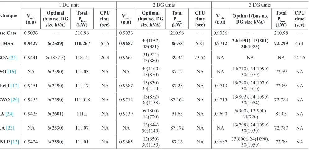
2. Case 2: P-Type DG
Table IV appendix (A) shows the optimal locations and capacities of PV units by the proposed GMSA method compared to different algorithms for the same three cases (1 DG, 2 DGs, and 3 DGs). The GMSA presented the best solutions as the power losses reduced to 110.267 kW with only one PV unit installed at bus 6. This value is considered the best value comparing with other techniques and also better than the all three cases of Q-type DG. Moreover, it enhanced the voltage profile as the minimum bus voltage at bus 18 increased from 0.9036 p.u to 0.9427 p.u. For 2 PV units case, the optimal bus places are at 13 and 30 for most methods. However, the proposed technique reduced the active power loss to 86.58 kW compared to 87.17 kW with PSO, 87.164 kW with HGWO, and 87.172 with EA. It is also observed from the results that the VD is enhanced to be 0.6723 p.u while the voltage stability is also enhanced to be 29.4035 p.u. In the last case of installing three PV units, GMSA selected buses 13, 24, and 30 to locate the PV units with 801, 1091, 1053 kW, respectively, which helps in reducing the real power loss to 72.299 kW and increasing the minimum bus voltage to 0.9712 p.u.
(a)
(b)
(c)
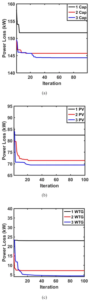
Fig. 4. Power loss convergence rate of 33-bus system using GMSA for different
DG types (a) Capacitor banks, (b) PV, (c) WTG.
These results prove the superiority of the proposed GMSA compared to other methods as seen in Table IV. It is also observed that the power loss is minimized significantly as compared with the Q-type DGs, this helps in improvement in the system voltage profile.
(a)
(b)
(c)
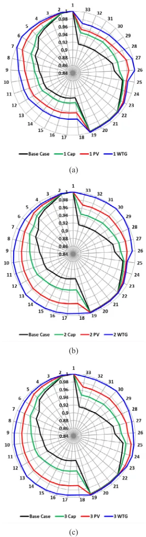
Fig. 5. 33-Bus voltage profile level with (a) Single DG (b) Two DGs (c) Three
DGs.
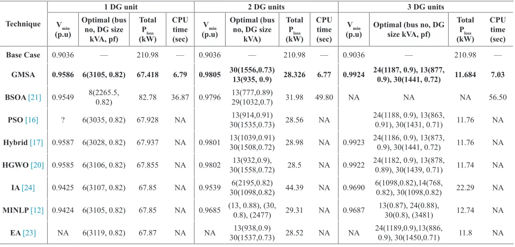
3. Case 3: PQ--Type DG
two WTG diminished the power losses to 28.33 kW, while three WTGs reduced it to 11.68 kW, which is the best-minimized power losses value for all cases of different DGs. Further, the voltage stability is enhanced to be 31.53 p.u and the VD is minimized to 0.1223 p.u.
For this case of 33 bus system, the GMSA, HGWO, and EA produce better solutions compared to the other methods, whereas the best power loss value obtained by BSOA is much more than the rest of algorithms. The GMSA has a speedy and smooth rate of convergence to the minimum value without any oscillations and settles down early as shown in Fig. 4. On the other hand, the WTG has the best effect on the system performance as one WTG gave better results than 3 units of capacitor banks or 3 PV units. Fig. 5(a, b, c) shows a comparison between the different types of DGs in terms of voltage profile improvement.
B. 69-Bus Test System
To investigate the effectiveness of the proposed GMSA on a large scale of RDN, it is applied on the 69-bus system, which consists of 69 buses and 68 branches as shown in Fig. 6. This system is operated with 100 MVA base, 12.66 kV rated voltage, and the total system load is (1.896MW+j1.347MVAR). All data of lines and loads are given in [35]. The total real power loss for the base case without using capacitors or DGs is found at 224.99 kW with the lowest bus voltage at bus 65 is 0.9092 p.u. The best locations and sizes of the three types of PV, WTG, and capacitor banks that are obtained by the proposed GMSA and all results are listed in Table VI appendix (A) in terms of power losses, minimum and maximum bus voltages, VD, VSI, and the percentage of loss reduction.
Fig. 6. Single line diagram of the 69-bus RDN [35].
1. Case 1: Q-Type DG
In this case, using the capacitors banks as Q-type helps in reducing the 69 bus system power loss by 32.61% from the base case using one DG unit at bus 61 with the size of 1200 kVAR, using the GMSA. It is considered the lowest value compared to the other methods. Moreover, the GMSA has increased the minimum bus voltage value to 0.9296 p.u after compensation. While, the power losses are reduced to 35.27% and 35.83% with two and three capacitors, respectively. Table VII appendix (A) summarized the obtained results by GMSA technique in case of installing 1 capacitor bank, 2 capacitor banks, and 3 capacitor banks units compared to other four algorithms. The results stated that as the number of capacitor banks units increased, the minimizing of power loss increased and consequently improved the whole system profile.
2. Case 2: P-Type DG
As for the previous system 33-bus, the installing of PV units enhances the voltage profile of the 69 bus system. It is seen from Table VIII appendix (A) that the GMSA selected bus 61 to install 1.87 MW PV unit, which reduces the power losses to 82.4 kW compared to 83.22 kW with MFO, HGWO and PSO, and 83.34 kW with EA. These four algorithms came in the second order after the GMSA method. While,
a hybrid approach, MINLP, and IA came after that with 83.37, 83.38 and 83.44 kW, respectively. Moreover, GMSA enhanced the minimum bus voltage from 0.9036 p.u to 0.9686 p.u. For 2 PV units, the optimal bus locations are the same at 17 and 61 for all the methods, except the GMSA at 15 and 61. The power loss is 71.37 kW by GMSA. It is the lowest of all techniques as seen in Table VIII. In the last case of installing three PV units, GMSA selected buses 11, 17, and 61 to place the PV units with 526, 380.7, 1718 kW, respectively, which helps in reducing the real power loss to 68.974 kW and increasing the minimum bus voltage to 0.9799 p.u. It is also observed from the results that the VD is enhanced to be 0.4471 p.u, while the voltage stability is also enhanced to be 66.2363 p.u.
(a)
(b)
(c)
(a)
(b)
(c)
Fig. 8. Power loss convergence rate of 69-bus system using different DG types
by GMSA.
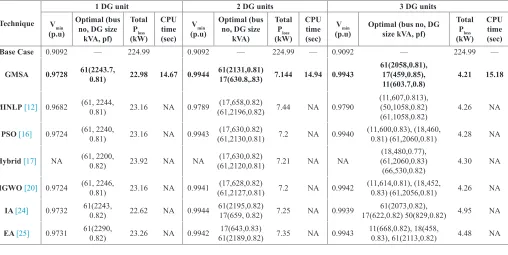
3. Case 3: PQ--Type DG
To verify the effectiveness of the proposed GMSA method, it has been applied to assign the best locations of one, two, and three WTGs. In case of inclusion of one WTG DG, the kW loss is reduced to 22.98 kW and the VD is enhanced to be 0.5825 p.u while the voltage stability is also enhanced to be 65.7382 p.u. Furthermore, it increased the minimum bus voltage to 0.9728 p.u. In this case, it can be seen from Table IX appendix (A) that the results of the GMSA are the best compared to all other methods in terms of power loss and minimum bus voltage. Further, it can be noted that the use of only one WTG is better than the usage of 3 capacitor banks or 3 PV units. Moreover, increasing the number of
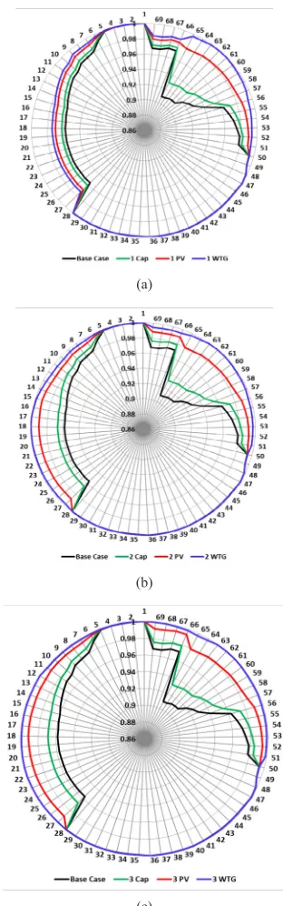
WTGs, leads to more reduction in power loss. The results stated that two WTG reduced the power losses to 7.144 kW, while three WTGs reduced it to 4.21 kW, which is the best-minimized power losses value for all cases and types of DGs. Further, the voltage stability is also enhanced to be 67.7559 p.u with minimizing the VD to 0.0617 p.u. The proposed hybrid algorithm provides a significant improvement of bus voltage profile and power loss in the case of PQ--type as compared with other cases. Fig. 7(a, b, c) shows a comparison between the different types of DGs in terms of voltage profile improvement.
The results stated that the GMSA method performed better than the other algorithms over all cases of the 69-bus system. In addition, the best performance of the proposed GMSA is noted by the flat and stable convergence curves of total real power losses as shown in Fig. 8.
V. Conclusion
In this article, the exploitation ability of the GMSA, in terms of quick convergence and fast execution time, has been maintained by using the best moths in the swarm to perform that role in the phases of the transverse orientation and celestial navigation. The tradeoff between the global and local search has been regulated by introducing an adaptive mutation operation of GA on the pathfinders as the largest population group in the swarm. In addition, individuals have cooperated to produce the light sources for the guidance of the transverse orientation phase, which assists the exploration ability in such exploitation phase and enhances the solution diversity. The complexity of reconnaissance phase has been reduced. The GA operations increased the information sharing and the performance of the proposed algorithm.
Appendix (A)
Nomenclature Pk Real power flow from bus k
Qk Reactive power flow from bus k
PLk Real power load connected at bus k
QLk Reactive power load connected at bus k
PL(k+1) Real power load connected at bus k+1
QL(k+1) Reactive power load connected at bus k+1
Rk Resistance connected between buses k and k+1
Xk Reactance connected between buses k and k+1
Vk Voltage at bus k
Vk+1 Voltage at bus k+1
Psys Network active power Qsys Network reactive power
ε1 Random samples drawn from Gaussian stochastic distribution Qfc Reactive power compensation
Vmin Minimum bus voltage value
Vmax Maximum bus voltage value PT loss Tap setting of transformer
np Number of pathfinders moths µt Variation coefficient
σ t
j Dispersal degree
bestg The global best solution
r1, r2 Random number within the interval [0, 1]
Pj The real power loss during jth load level n The number of candidate buses
Qfc The size of the shunt capacitor
ε2, ε3 Random numbers distributed uniformly within the interval [0,1]
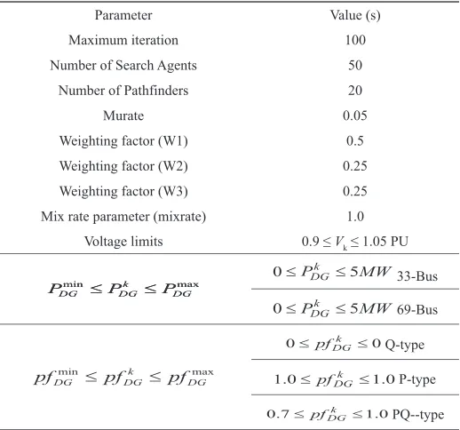
TABLE I. Control-Parameters Values for the Different Algorithms
Parameter Value (s)
Maximum iteration 100
Number of Search Agents 50
Number of Pathfinders 20
Murate 0.05
Weighting factor (W1) 0.5
Weighting factor (W2) 0.25
Weighting factor (W3) 0.25
Mix rate parameter (mixrate) 1.0 Voltage limits 0.9 ≤ Vk ≤ 1.05 PU
33-Bus
69-Bus
Q-type
P-type
TABLE II. Optimal Locations and Rating of Renewable DGs for Units Using GMSA for 33-Bus System
Type Vmin (p.u) (p.u)*Vmax Ploss (kW) reduction% Loss VSI (p.u) (p.u)VD Optimal bus no, optimal DG (kVA), optimal (pf)
Without DG 0.9036 0.9971 210.98 –– 25.5401 1.8044 ––
1 DG 1 Cap1 PV
1 WT
0.9175 0.9976 150.426 28.7% 26.7764 1.4259 30(1200)
0.9427 0.9980 110.267 47.74% 28.6451 0.9235 6(2589)
0.9586 1.000 67.418 68.05% 29.8458 0.5646 6(3105), (0.82)
2 DG 2 Cap2 PV
2 WT
0.9332 0.9978 140.876 33.23% 27.2855 1.2702 30(1050), 12(450)
0.9687 0.9984 86.58 58.96% 29.4035 0.6723 30(1157), 13(851)
0.9805 1.0009 28.326 86.57 31.2752 0.1867 30(1556, 0.73), 13(935, 0.9)
3 DG 3 Cap3 PV
3 WT
0.9334 0.9979 137.466 34.84% 27.3357 1.2568 24(450), 12(450), 30(1050) 0.9712 0.9989 72.299 65.73% 29.6328 0.6124 24(1091), 13(801), 30(1053) 0.9924 1.0006 11.684 94.46% 31.5347 0.1223 24(1187, 0.9), 13(877, 0.9), 30(1441, 0.72)
TABLE III. Comparison Results of Different Optimization Techniques for Q-type DG Units for 33-Bus System
Technique
1 DG unit 2 DG units 3 DG units
Vmin
(p.u)
Optimal (bus no, DG
size kVA)
Total Ploss (kW)
CPU time (sec)
Vmin
(p.u)
Optimal (bus no, DG
size kVA)
Total Ploss (kW)
CPU time (sec)
Vmin
(p.u) Optimal (bus no, DG size kVA)
Total Ploss (kW)
CPU time (sec)
Base Case 0.9036 –– 210.98 –– 0.9036 –– 210.98 –– 0.9036 –– 210.98 ––
GMSA 0.9175 30(1200) 150.426 6.2 09332 30(1050) 12(450) 140.87 6.22 0.9334 24(450), 12(450) 30(1050) 137.46 6.26
GA 0.9173 29(1350) 153.121 7.31 0.9159 30(1200)21(150) 151.12 7.34 0.9333 6(750), 13(350) 31(750) 142.07 7.48
MSA 0.9159 30(1200) 151.497 6.51 0.9297 30(900)8(750) 143.11 6.67 0.9298 2(150), 12(1050) 30(450) 141.71 6.93
Hybrid [17] 0.9161 30(1230) 151.41 NA 0.9336 30(1040) 12(430) 141.94 NA 0.9335 24(450), 12(450) 30(1050) 138.37 NA
HGWO [20] 0.9163 30(1258) 151.36 NA 0.9338 30(1054) 12(467) 141.83 NA 0.9334 24(450), 12(450) 30(1050) 138.25 NA
TABLE IV. Comparison Results of Different Optimization Techniques for P-Type DG Units for 33-Bus System
Technique
1 DG unit 2 DG units 3 DG units
Vmin
(p.u)
Optimal (bus no, DG
size kVA)
Total Ploss
(kW)
CPU time (sec)
Vmin
(p.u)
Optimal (bus no, DG
size kVA)
Total Ploss
(kW)
CPU time (sec)
Vmin
(p.u) Optimal (bus no, DG size kVA) Total
Ploss
(kW) CPU time (sec)
Base Case 0.9036 –– 210.98 –– 0.9036 –– 210.98 –– 0.9036 –– 210.98 ––
GMSA 0.9427 6(2589) 110.267 6.55 0.9687 30(1157) 13(851) 86.58 6.81 0.9712 24(1091), 13(801) 30(1053) 72.299 6.61
BSOA [21] 0.9441 8(1857.5) 118.12 20.4 0.9665 31(924) 13(880) 89.34 23.54 NA NA NA 24.95
PSO[16] NA 6(2590) 111.03 NA NA 30(1160) 13(850) 87.17 NA NA 14(770), 24(1090) 30(1070) 72.79 NA
Hybrid [17] 0.9451 6(2490) 111.17 NA 0.9687 30(1110)13(830) 87.28 NA 0.9713 13(790), 24(1070) 30(1010) 72.89 NA
HGWO [20] 0.9455 6(2590) 111.018 NA 0.9714 30(1158)13(852) 87.164 NA 0.9715 13(802), 24(1090) 30(1054) 72.784 NA
IA [24] 0.9425 6(2601) 111.1 NA 0.9539 6(1800) 14(720) 91.63 NA 0.9690 6(900), 12(900) 31(720) 81.05 NA
EA [23] NA 6(2530) 111.07 NA NA 30(1149)13(844) 87.172 NA NA 13(798), 24(1099) 30(1050) 72.787 NA
TABLE V. Comparison Results of Different Optimization Techniques for PQ--type DG Units for 33-Bus System
Technique
1 DG unit 2 DG units 3 DG units
Vmin (p.u)
Optimal (bus no, DG size
kVA, pf)
Total Ploss
(kW) CPU time (sec)
Vmin (p.u)
Optimal (bus no, DG size
kVA)
Total Ploss
(kW) CPU time (sec)
Vmin
(p.u) Optimal (bus no, DG size kVA, pf) Total
Ploss
(kW)
CPU time (sec)
Base Case 0.9036 –– 210.98 –– 0.9036 –– 210.98 –– 0.9036 –– 210.98 ––
GMSA 0.9586 6(3105, 0.82) 67.418 6.79 0.9805 30(1556,0.73) 13(935, 0.9) 28.326 6.77 0.9924 24(1187, 0.9), 13(877, 0.9), 30(1441, 0.72) 11.684 7.03
BSOA [21] 0.9549 8(2265.5, 0.82) 82.78 36.87 0.9796 13(777,0.89) 29(1032,0.7) 31.98 49.80 NA NA NA 56.50
PSO[16] ? 6(3035, 0.82) 67.928 NA 30(1535,0.73)13(914,0.91) 28.56 NA 24(1188, 0.9), 13(863, 0.91), 30(1431, 0.71) 11.76 NA
Hybrid[17] 0.9587 6(3028, 0.82) 67.937 NA 0.9801 13(1039,0.91) 30(1508,0.72) 28.98 NA 0.9923 24(1186, 0.9), 13(873, 0.9), 30(1441, 0.72) 11.76 NA
HGWO [20] 0.9585 6(3106, 0.82) 67.855 NA 0.9802 30(1558,0.72)13(932,0.9), 28.5 NA 0.9922 24(1182, 0.9), 13(878, 0.89), 30(1439, 0.71) 11.74 NA
IA [24] 0.9425 6(3107, 0.82) 67.85 NA 0.9539 30(1098,0.82)6(2195,0.82) 44.39 NA 0.9690 6(1098,0.82),14(768, 0.82), 30(1098,0.82) 22.29 NA
MINLP [12] 0.9424 6(3105, 0.82) 67.85 NA 0.9685 (13, 0.88), (30, 0.8), (2477) 29.31 NA 0.9687 13(0.87), 24(0.88), 30(0.8), (3481) 12.74 NA
EA [23] NA 6(3119, 0.82) 67.87 NA NA 30(1537,0.73)13(938,0.9) 28.52 NA NA 24(1189,0.9),13(886, 0.9), 30(1450,0.71) 11.8 NA
TABLE. VI. Optimal Locations and Rating of Renewable DGs for Units Using GMSA for 69-Bus System
Type Vmin (p.u) Vmax (p.u)* Ploss (kW) reduction% Loss VSI (p.u) VD (p.u) Optimal bus no, optimal DG (kVA), optimal (pf)
Without DG 0.9092 0.9999 224.99 –– 61.2183 1.8374 ––
1 DG 1 Cap1 PV
1 WT
0.9296 0.9999 151.617 32.61% 62.2409 1.5361 61(1200)
0.9686 0.9999 82.4 63.38% 64.6524 0.8645 61(1872)
0.9728 0.9999 22.98 89.79% 65.7382 0.5825 61(2243.7, 0.81)
2 DG 2 Cap2 PV
2 WT
0.9315 0.9999 145.646 35.27% 62.6248 1.4293 61(1200), 12(600)
0.9792 0.9999 71.371 68.28% 66.0147 0.5041 61(1777), 15(554)
0.9944 1.0003 7.144 96.82% 67.4868 0.1289 61(2131, 0.81), 17(630.8, 0.83)
3 DG 3 Cap3 PV
3 WT
0.9318 0.9999 144.369 35.83% 62.7862 1.3844 61(1200), 53(350), 17(350) 0.9799 1.0002 68.974 69.34% 66.2363 0.4471 61(1718), 17(380.7), 11(526) 0.9943 1.003 4.21 98.13% 67.7559 0.0617 61(2058,0.81), 17(459,0.85), 11(603.7,0.8)
TABLE. VII. Comparison Results of Different Optimization Techniques for Q-type DG Units for 69-Bus System
Technique
1 DG unit 2 DG units 3 DG units
Vmin (p.u)
Optimal (bus no, DG size
kVA)
Total Ploss
(kW)
CPU time (sec)
Vmin (p.u)
Optimal (bus no, DG size
kVA)
Total Ploss
(kW)
CPU time (sec)
Vmin
(p.u) Optimal (bus no, DG size kVA) Total
Ploss
(kW)
CPU time (sec)
Base Case 0.9092 –– 224.99 –– 0.9092 –– 224.99 0.9092 –– 224.99
GMSA 0.9312 61(1200) 151.617 14.3 0.9315 61(1200) 12(600) 145.65 13.76 0.9318 61(1200) 53(350), 17(350) 144.37 14.66
GA [29] 0.9311 61(1350) 152.07 NA 0.9310 61(1200) 66(600) 147.63 NA 0.9308 12(600), 45(150) 61(1200) 146.72 NA
MSA [29] 0.9310 61(1350) 152.05 NA 0.9288 61(1200) 12(600) 146.69 NA 0.9299 2(1050), 17(350) 61(1200) 146.61 11.42
Hybrid [17] NA 61(1290) 152.1 NA NA 61(1240) 18(350) 146.49 NA NA 11(330), 18(250) 61(1190) 145.28 NA
References
[1] P. Dinakara, V. C. Veera, and T. Gowri Manohar, “Whale optimization algorithm for optimal sizing of renewable resources for loss reduction in distribution systems”, Renewable: Wind, Water, and Solar, Vol. 4, No.1, 2017, pp. 1.
[2] L. Freris, D. Infield, Renewable energy in power system. Wiltshire: A John Wiley & Sons; 2008.
[3] M. Saejia and I. Ngamroo “Stabilization of microgrid with intermittent renewable energy sources by SMES with optimal coil size”, Elsevier,
Physica C, 2011, pp. 1385–1389.
[4] HA, M. P., Huy, P. D., & Ramachandaramurthy, V. K. “A review of the optimal allocation of distributed generation: Objectives, constraints, methods, and algorithms”. Renewable and Sustainable Energy Reviews, 75, 2017, pp. 293-312.
[5] T. Griffin, K. Tomsovic, D. Secrest, A. Law, “Placement of dispersed generation systems for reduced losses. In: 33th proceeding Hawaii int. Conf. on System sciences”, 2000. pp. 1-9.
[6] W. Ahmed, A. Selim, S. Kamel, J. Yu, F. Jurado, “Probabilistic Load Flow
Solution Considering Optimal Allocation of SVC in Radial Distribution System”, International Journal of Interactive Multimedia and Artificial
Intelligence. 2018;5(3):152-161.
[7] N. Rezaei, MR.Haghifam, “Protection Scheme for A Distribution system with distributed generation using neural networks”, Int. J Electr Power
Energy Syst, May 2008;30(4):235-241.
[8] TJ. Hashim, A. Mohamed, “Fuzzy logic based coordinated voltage control for distribution network with distributed generations”, Int. J. of Electrical,
Computer, Energetic, Electron Commun Eng 2013;7(7):369-374.
[9] A. Awad, T. El-Fouly, M. Salama, “Optimal distributed generation allocation and load shedding for improving distribution system reliability”,
Electr Power Components Syst, 2014;42(6):576-584.
[10] F. S. Abu-Mouti and M. El-Hawary, “Optimal distributed generation allocation and sizing in distribution systems via artificial bee colony algorithm,” IEEE transactions on power delivery, vol. 26, 2011, pp. 2090-2101.
[11] T. Shukla, S. Singh, V. Srinivasarao, and K. Naik, “Optimal sizing of distributed generation placed on radial distribution systems,” Electric
power components and systems, vol. 38, pp. 260-274, 2010.
TABLE. VIII. Comparison Results of Different Optimization Techniques for P-type DG Units for 69-Bus System
Technique
1 DG unit 2 DG units 3 DG units
Vmin (p.u)
Optimal (bus no, DG size
kVA)
Total Ploss
(kW)
CPU time (sec)
Vmin (p.u)
Optimal (bus no, DG size
kVA)
Total Ploss
(kW) CPU
time (sec)
Vmin
(p.u) Optimal (bus no, DG size kVA)
Total Ploss
(kW)
CPU time (sec)
Base Case 0.9092 –– 224.99 –– 0.9092 –– 224.99 –– 0.9092 –– 224.99 ––
GMSA 0.9686 61(1872) 82.4 14.66 0.9792 61(1777) 15(554) 71.371 14.3 0.9799 17(380.7), 11(526)61(1718) 68.974 14.69
IA [24] 0.9692 61(1900) 83.44 NA 0.9765 61(1700) 17(510) 72.13 NA 0.9785 11(340), 17(510) 61(1700) 70.16 NA
PSO[16] 0.9681 61(1870) 83.222 NA 0.9806 17(1780) 61(1530) 71.68 NA 0.9806 11(460), 17(440) 61(1700) 69.52 NA
Hybrid [17] NA 61(1810) 83.372 NA NA 61(1720)17(520) 71.82 NA NA 12(496), 22(311) 61(1735) 69.56 NA
HGWO[20] 0.9682 61(1872) 83.222 NA 0.9799 61(1781)17(531) 71.674 NA 0.9799 11(527), 17(380) 61(1781) 69.425 NA
MINLP [12] 0.9682 61(1870) 83.38 NA 0.9789 61(1780)17(530) 71.83 NA 0.9790 11(530), 17(380) 61(1720) 69.59 NA
EA[23] NA 61(1878) 83.23 NA NA 61(1795)17(534) 71.68 NA NA 11(467), 18(380) 61(1795) 69.62 NA
TABLE. IX. Comparison Results of Different Optimization Techniques for PQ--type DG Units for 69-Bus System
Technique
1 DG unit 2 DG units 3 DG units
Vmin (p.u)
Optimal (bus no, DG size
kVA, pf)
Total Ploss (kW)
CPU time (sec)
Vmin (p.u)
Optimal (bus no, DG size
kVA)
Total Ploss (kW)
CPU time (sec)
Vmin
(p.u) Optimal (bus no, DG size kVA, pf)
Total Ploss (kW)
CPU time (sec)
Base Case 0.9092 –– 224.99 0.9092 –– 224.99 –– 0.9092 –– 224.99 ––
GMSA 0.9728 61(2243.7, 0.81) 22.98 14.67 0.9944 61(2131,0.81) 17(630.8,.83) 7.144 14.94 0.9943 61(2058,0.81), 17(459,0.85),
11(603.7,0.8) 4.21 15.18
MINLP[12] 0.9682 (61, 2244, 0.81) 23.16 NA 0.9789 (17,658,0.82) (61,2196,0.82) 7.44 NA 0.9790 (11,607,0.813), (50,1058,0.82)
(61,1058,0.82) 4.26 NA
PSO [16] 0.9724 (61, 2240, 0.81) 23.16 NA 0.9943 (17,630,0.82) (61,2130,0.81) 7.2 NA 0.9940 (11,600,0.83), (18,460, 0.81) (61,2060,0.81) 4.28 NA
Hybrid [17] NA (61, 2200, 0.82) 23.92 NA NA (61,2120,0.81)(17,630,0.82) 7.21 NA NA (61,2060,0.83) (18,480,0.77),
(66,530,0.82) 4.30 NA
HGWO [20] 0.9724 (61, 2246, 0.81) 23.16 NA 0.9941 (17,628,0.82) (61,2127,0.81) 7.2 NA 0.9942 (11,614,0.81), (18,452, 0.83) (61,2056,0.81) 4.26 NA
IA [24] 0.9732 61(2243, 0.82) 22.62 NA 0.9944 61(2195,0.82) 17(659, 0.82) 7.25 NA 0.9939 17(622,0.82) 50(829,0.82)61(2073,0.82), 4.95 NA
[12] W. Tan, M. Hassan, M. Majid, and H. A. Rahman, “Allocation and sizing of DG using Cuckoo Search algorithm,” in Power and Energy (PECon), 2012 IEEE International Conference on, 2012, pp. 133-138.
[13] S. Kaur, G. Kumbhar, and J. Sharma, “A MINLP technique for optimal placement of multiple DG units in distribution systems,” International
Journal of Electrical Power & Energy Systems, vol. 63, Dec. 2014, pp.
609-617.
[14] L. Arya, A. Koshti, and S. Choube, “Distributed generation planning using differential evolution accounting voltage stability consideration,”
International Journal of electrical power & energy systems, vol. 42, pp.
196-207, 2012.
[15] E. S. Oda, A. A. Abdelsalam, M. N. Abdel-Wahab, and M. M. El-Saadawi, “Distributed generations planning using flower pollination algorithm for enhancing distribution system voltage stability,” Ain Shams Engineering
Journal, 2015.
[16] S. K. Injeti at al., “A novel approach to identify optimal access point and capacity of multiple DGs in a small, medium and large-scale radial distribution systems,” Int. Journal of Electrical Power & Energy Systems, vol. 45, no. 1, Feb. 2013, pp. 142-151.
[17] B.B. Zad, H. Hasanvand, J. Lobry, and F. Vallée, “Optimal reactive power control of DGs for voltage regulation of MV distribution systems using sensitivity analysis method and PSO algorithm,” International Journal of
Electrical Power & Energy Systems, vol. 68, Jun. 2015, pp. 52-60.
[18] S. Kansal, V. Kumar, and B. Tyagi, “Hybrid approach for optimal placement of multiple DGs of multiple types in distribution networks,”
International Journal of Electrical Power & Energy Systems, vol. 75, Feb.
2016, pp. 226-235.
[19] M.H. Moradi, A. Zeinalzadeh, Y. Mohammadi, and M. Abedini, “An efficient hybrid method for solving the optimal siting and sizing problem of DG and shunt capacitor banks simultaneously based on an imperialist competitive algorithm and genetic algorithm,” International Journal of
Electrical Power & Energy Systems, vol. 54, Jan. 2014, pp. 101-111.
[20] M. Kefayat, A.L. Ara, and S.N. Niaki, “A hybrid of ant colony optimization and artificial bee colony algorithm for probabilistic optimal placement and sizing of distributed energy resources,” Energy Conversion and
Management, vol. 92, Mar. 2015, pp.149-161.
[21] R. Sanjay, Jayabarathi, T. Raghunathan, V. Ramesh, and Nadarajah, “Optimal Allocation of Distributed Generation Using Hybrid Grey Wolf Optimizer”, IEEE Access, 2017, pp. 14807 – 14818.
[22] El-Fergany A. Optimal allocation of multi-type distributed generators using backtracking search optimization algorithm. Int. J Electr Power
Energy Syst. Vol. 64, January 2015, pp. 1197-1205.
[23] K. Muthukumar, and S. Jayalalitha, “Optimal placement and sizing of distributed generators and shunt capacitors for power loss minimization in radial distribution networks using hybrid heuristic search optimization technique,” International Journal of Electrical Power & Energy Systems, vol. 78, Jun. 2016, pp. 299-319.
[24] K. Mahmoud, N. Yorino, and A. Ahmed, “Optimal distributed generation allocation in distribution systems for loss minimization,” IEEE
Transactions on Power Systems, vol. 31, no. 2, Mar. 2016, pp. 960-969.
[25] D.Q. Hung, and N. Mithulananthan, “Multiple distributed generator placement in primary distribution networks for loss reduction,” IEEE Transactions on
industrial electronics, vol. 60, no. 4, Apr. 201, pp. 1700-1708.
[26] K. Mahmoud and M. Abdel-Nasser, “Fast-yet-Accurate Energy Loss Assessment Approach for Analyzing/Sizing PV in Distribution Systems Using Machine Learning,” IEEE Transactions on Sustainable Energy, vol. 10, no. 13, July. 2019, pp. 1025-1033.
[27] Naresh Acharya, Pukar Mahat, N. Mithulananthan, “An analytical approach for DG allocation in primary distribution network”, Electrical
Power and Energy Systems, vol. 28, 2006, pp. 669-678.
[28] E. Ali, S. A. Elazim, and A. Abdelaziz, “Ant Lion Optimization Algorithm for Renewable Distributed Generations,” Energy, vol. 116, pp. 445-458, 2016.
[29] A. El-Fergany, “Optimal allocation of multi-type distributed generators using backtracking search optimization algorithm,” International Journal
of Electrical Power & Energy Systems, vol. 64, pp. 1197-1205, 2015.
[30] Mohamed, E. A., Mohamed, A. A. A., & Mitani, Y, “Hybrid GMSA for Optimal Placement and Sizing of Distributed Generation and Shunt Capacitors,” Journal of Engineering Science & Technology Review, 11(1).
[31] EA. Mohamed, A. Mohamed -, and Y. Mitani, “MSA for Optimal Reconfiguration and Capacitor Allocation in Radial/Ring Distribution Networks,” International Journal of Interactive Multimedia and Artificial
Intelligence. 2018;5(1):107-122.
[32] J. A. Micheline Ruba and S. Ganesh “Power Flow Analysis for Radial Distribution Systems using Backward/Forward Sweep Method”,
International Journal of Electrical and Computer Engineering, Vol 8,
No.10, 2014, pp. 1621 – 1625.
[33] W.Sheng, K. Y. Liu, Y. Liu, X. Meng, and Y. Li, “Optimal placement and sizing of distributed generation via an improved nondominated sorting genetic algorithm II,” IEEE Transactions on Power Delivery, 2015, 30(2), 569-578.
[34] B. Venkatesh, and R. Ranjan, “Optimal radial distribution system reconfiguration using fuzzy adaptation of evolutionary programming,”
International journal of electrical power & energy systems, vol. 25, no.
10, pp. 775-780, Dec. 2013.
[35] J.S. Savier, and D. Das, “Impact of network reconfiguration on loss allocation of radial distribution systems,” IEEE Transactions on Power
Delivery, vol. 22, no. 4, pp. 2473-2480, Oct 2007.
Emad A. Mohamed
He received the B.Sc., M.Sc. and PhD degrees in electrical power engineering from Aswan University, Aswan, Egypt, and Kyushu Institute of Technology in 2005, 2013, and 2019 respectively. He was working as a Demonstrator in the Department of Electrical Engineering, Aswan Faculty of Engineering, Aswan University, Aswan, Egypt. Between November 2007 and August 2013, and he is an assistant lecturer from 2013 to 2019. Now, he is an Assistant Professor. He was in a Master Mobility scholarship at Faculté des Sciences et Technologies - Université de Lorraine, France – 1. The scholarship sponsored by FFEEBB ERASMUS MUNDUS. He was a research student from April to October 2015 in Kyushu University, Japan. His research interests are applications of superconductivity on power systems, power system stability, and protection.
Al-Attar Ali Mohamed
Al-Attar Ali Mohamed received his B.Eng., M.Eng, and Ph.D. from Aswan University, Aswan, Egypt in 2010, 2013 and 2017. Currently, he is an assistant professor sponsored in Faculty of Engineering, Aswan University. His research interests are in the area of analysis and design of power systems, optimization, and controls.
Yasunori Mitani
![Fig. 3. Single line diagram of the 33-bus RDN [34].](https://thumb-us.123doks.com/thumbv2/123dok_us/9702968.1953494/5.612.51.296.511.625/fig-single-line-diagram-of-the-bus-rdn.webp)