557 Information Technology and Control 2019/4/48
Model Predictive Control of
UCG: An Experiment and
Simulation Study
ITC 4/48 Information Technology and Control
Vol. 48 / No. 4 / 2019 pp. 557-578
DOI 10.5755/j01.itc.48.4.23303
Model Predictive Control of UCG: An Experiment and Simulation Study
Received 2019/04/30 Accepted after revision 2019/10/21
http://dx.doi.org/10.5755/j01.itc.48.4.23303
Corresponding author: [email protected]
Ján Kačur, Patrik Flegner, Milan Durdán, and Marek Laciak
Faculty of Mining, Ecology, Process Control, and Geotechnologies; Institute of Control and Informatization of Production Processes, Technical University of Košice, Němcovej 3, 040 01 Košice, Slovak Republic;
e-mail: [email protected]
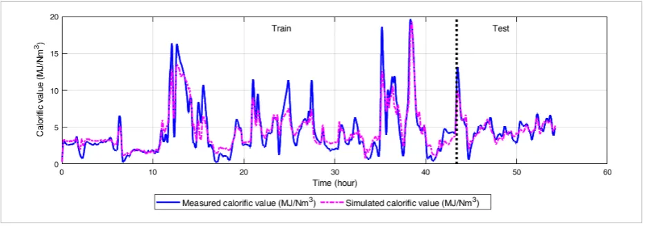
Underground coal gasification (UCG) is a potential technology that enables to mine coal without traditional mining equipment. The coal is gasified deep in underground and produced syngas is processed on the surface. The most important technical problem in UCG is unstable quality of syngas and control. This paper propos-es advanced control based on an adaptive predictive controller. The maintaining of dpropos-esired calorific value de-pends on flow rates of gasification agents injected to the underground geo-reactor and controlled exhaust. The paper proposes a physical model of UCG technology and applies a method of multivariate adaptive regression splines (MARS) to model the gasification process. This method satisfactorily approximates nonlinearity in the process variables. The paper proposes adaptive model predictive control (MPC) using online model estimation and applied it on the MARS model of UCG that imitates the real process. The results have shown that optimiza-tion of manipulaoptimiza-tion variables can replace manual control in UCG. Getting better quality of syngas depends on setpoints, optimized manipulation variables, and constraints used in MPC. In simulations, the adaptive MPC has shown better performance in comparison with manual and PI control.
KEYWORDS: UCG, Coal, Gasification, Prediction, Model Predictive Control, MARS, Matlab-Simulink.
1. Introduction
Underground coal gasification (UCG) represents in-situ controlled combustion of coal where valuable gas (i.e., syngas) is produced. Conventional mining
Information Technology and Control 2019/4/48 558
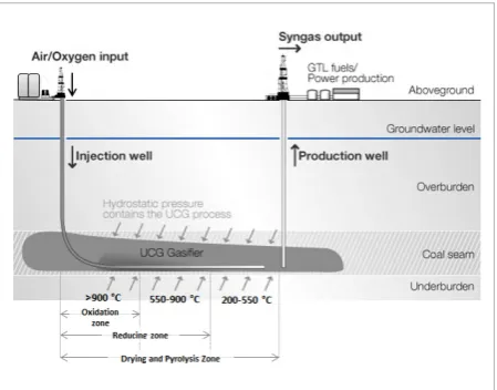
not mineable by conventional approach or have some tectonic failures. Moreover, it is less expensive than traditional mining. UCG has the potential to be used in the future. In in-situ gasification two wells drilled into underground are needed to initiate gasification, i.e., injection and production well. In UCG, heat is generated in the underground coal bed using injected oxidants (i.e., by endothermic chemical reactions). This heat is used by exothermic reactions with car-bon to produce syngas components. With the need to improve the gasification process, it must be ensured that the combustive reactions have generated enough energy to heat of reactants. The calorific value of the produced syngas is the most important indicator of gasification quality. In UCG, various gasification agents are used, e.g., air, oxygen, or water vapor. In an underground reactor, the processes of drying, pyrol-ysis of solid hydrocarbon, combustion and gasifica-tion continually take place. UCG represents reacgasifica-tion zones defined by temperatures where the combustion front progressively moves. Groundwater also partic-ipates in gasification. Raw, pure syngas from UCG contains predominantly CO, CO2, H2, CH4, and O2, higher hydrocarbons, tar, and impurities. Monitoring the underground temperature in the oxidation zone is important for the control of UCG. The UCG runs in temperatures close to 1000°C according to Figure 1. At the fire face, there are high temperatures (up to 1200–1300°C). An extensive overview of UCG can be found in [9, 12, 39].
Figure 1
Principle of the UCG with reaction zones
heat is used by exothermic reactions with carbon to produce syngas components. With the need to improve the gasification process, it must be ensured that the combustive reactions have generated enough energy to heat of reactants. The calorific value of the produced syngas is the most important indicator of gasification quality. In UCG, various gasification agents are used, e.g., air, oxygen, or water vapor. In an underground reactor, the processes of drying, pyrolysis of solid hydrocarbon, combustion and gasification continually take place. UCG represents reaction zones defined by temperatures where the combustion front progressively moves. Groundwater also participates in gasification. Raw, pure syngas from UCG contains predominantly CO, CO2, H2, CH4, and O2, higher
hydrocarbons, tar, and impurities. Monitoring the underground temperature in the oxidation zone is important for the control of UCG. The UCG runs in temperatures close to 1000°C according to Figure 1. At the fire face, there are high temperatures (up to 1200–1300°C). An extensive overview of UCG can be found in [9, 12, 39].
Figure 1
Principle of the UCG with reaction zones.
Research in the world is mainly focused on modeling internal processes of UCG and on model-based control. This paper examines the possibilities of model predictive control of UCG with adapted internal controller model. In this paper, the simulation study is performed to assess the suitability of the proposed approach. Major contributions of this paper are as follows: 1) A data-driven modeling of syngas calorific value and underground temperature by utilizing the model based on multivariate adaptive regression splines (MARS). The MARS model will be used to imitate the UCG process in simulations. Such an approach
has not yet been applied in the world; 2) A proposal of the adaptive predictive control to maintain or increase the syngas calorific value. Such an approach to UCG control has not yet been verified. 3) A comparison of the proposed predictive control with manual control and classical PI control. The following subsections give an overview of recent research in the field of UCG modeling and control.
1.1 UCG Modeling
The UCG involves a complex range of physical processes occurring over a wide range of characteristic time and length scales. Modeling of such processes is a compromise between model complexity (often assumed to give better predictive capability) versus simplicity (known to provide faster computational runtimes). The tradeoffs made in the model development are typically a function of the model's intended purpose, expectations of the uncertainties, and sensitivities of model inputs the current state-of-knowledge and the available computing power. A comprehensive UCG model should include various physical phenomena (e.g., heat and mass transfers, coal drying and pyrolysis, chemical reactions cavity evolution, liquid flow and interaction between surrounding environment) and physical sub-processes (e.g., cavity growth, combustion front propagation, the interaction of the cavity with overburden and hydrology) [45]. In the literature, different approaches to UCG modeling can be found. Earliest numerical models were one-dimensional packed bed [40, 57]. Thorsness et al. [49] were able to make a good prediction of syngas composition and coal consumption for laboratory experiments with steam and oxygen (ratio 6:1). Later, 2-D packed bed and channel models were developed [1, 4, 50]. For thick seams with low-pressure operations (< 1 MPa), a CAVSIM process was developed [48]. Progress in computing has enabled the development of 3-D models of UCG, e.g., a 3-D computational model for roof spalling, bed dynamics, and cavity growth were developed in [5]. An important aspect of UCG models are the assumptions and modeling of the chemical reactions in the process. Models based on a chemical reaction of UCG can be found in [8, 47]. The comprehensive summary of reported UCG models can be found in [27, 45].
A special group consists of mathematical models based on soft sensors where an unmeasurable process variable is calculated or estimated from
Research in the world is mainly focused on model-ing internal processes of UCG and on model-based control. This paper examines the possibilities of model predictive control of UCG with adapted in-ternal controller model. In this paper, the simula-tion study is performed to assess the suitability of the proposed approach. Major contributions of this paper are as follows: 1) A data-driven modeling of syngas calorific value and underground temperature by utilizing the model based on multivariate adap-tive regression splines (MARS). The MARS model will be used to imitate the UCG process in simula-tions. Such an approach has not yet been applied in the world; 2) A proposal of the adaptive predictive control to maintain or increase the syngas calorific value. Such an approach to UCG control has not yet been verified. 3) A comparison of the proposed pre-dictive control with manual control and classical PI control. The following subsections give an overview of recent research in the field of UCG modeling and control.
1.1. UCG Modeling
The UCG involves a complex range of physical pro-cesses occurring over a wide range of characteristic time and length scales. Modeling of such processes is a compromise between model complexity (often assumed to give better predictive capability) versus simplicity (known to provide faster computational runtimes). The tradeoffs made in the model develop-ment are typically a function of the model’s intended purpose, expectations of the uncertainties, and sen-sitivities of model inputs the current state-of-knowl-edge and the available computing power.
A comprehensive UCG model should include various physical phenomena (e.g., heat and mass transfers, coal drying and pyrolysis, chemical reactions cavity evolution, liquid flow and interaction between sur-rounding environment) and physical sub-processes (e.g., cavity growth, combustion front propagation, the interaction of the cavity with overburden and hy-drology) [45].
ex-559 Information Technology and Control 2019/4/48
periments with steam and oxygen (ratio 6:1). Later, 2-D packed bed and channel models were developed [1, 4, 50]. For thick seams with low-pressure oper-ations (< 1 MPa), a CAVSIM process was developed [48]. Progress in computing has enabled the develop-ment of 3-D models of UCG, e.g., a 3-D computation-al model for roof spcomputation-alling, bed dynamics, and cavity growth were developed in [5]. An important aspect of UCG models are the assumptions and modeling of the chemical reactions in the process. Models based on a chemical reaction of UCG can be found in [8, 47]. The comprehensive summary of reported UCG models can be found in [27, 45].
A special group consists of mathematical models based on soft sensors where an unmeasurable pro-cess variable is calculated or estimated from other measurable process variables. Since the UCG runs in the underground, some of the process variables can-not be measured directly by conventional hardware (e.g., underground temperature). Known proxies of underground temperature estimation are based on measurement of carbon isotopes [11, 28] and radon emanations [54, 58]. Various soft-sensing methods are developed for monitoring and prediction of UCG variables. Currently, UCG modeling with the appli-cation of machine learning (i.e., neural networks (NNs), support vector machines (SVMs), and adap-tive regression models) is developed. This approach brings interesting results in the modeling of expert knowledge of the UCG. It is mostly data-driven modeling with continuous model adaptation as the process evolves. In terms of control, it needs to pre-dict the composition of syngas calorific value, or un-derground temperature in a combination of control variables.
Some works model underground temperature based on nonstationary heat conduction (e.g., [17, 29]). Re-cently, many models based on neural networks were developed (e.g., [23, 26, 35, 36]). Some models are di-rectly developed to support predictive control. Vari-ous applications of support vector machines (SVMs) for UCG data prediction can be found in the litera-ture. For example, Kačur et al. [25] achieved interest-ing results in predictinterest-ing calorific value usinterest-ing support vector regression (SVR). Other methods of prediction applied in UCG that utilize soft computing can be found in [22, 37, 60, 61].
1.2. Control of UCG
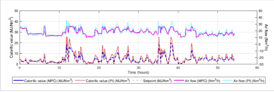
The control of UCG to produce stable syngas is most problematic. Currently, the UCG is controlled blindly, causing unstable quality of syngas. For air technology (i.e., the air is used as a main gasification agent), a low-er syngas calorific value of 3-7 MJ/Nm3 is achieved. In oxygen technology (i.e., typically a mixture of oxy-gen and water vapor), the calorific value is usually in the range of 9-14 MJ/Nm3 [39]. Optimal control is the most investigated field in UCG within academic re-search. Much work focused on UCG control has been done on experimental ex-situ reactors (e.g., [24, 30, 31]) but also there are some trials on in-situ gasifier (e.g., [52]).
The discrete PI controller is ideal for slow and time-delayed processes such as UCG. Applications of PI controllers to stabilize the oxygen in syngas and underground temperature can be found in [24]. Kačur and Kostúr proposed PI controllers using discrete ARX models and a modified Ziegler-Nichols method [24]. The authors also verified the PI controller with a continuous adaptation of controller parameters. By such an approach, they were able to increase and maintain the syngas calorific value. Another approach to automated UCG control was based on the applica-tion of the adaptive regression model [33]. The pro-posed regression model was able to calculate optimal manipulation variables (i.e., volume flows of gasifica-tion agents) with the continual adaptagasifica-tion of model parameters from the historical data. Recently, Kostúr and Kačur [30] developed optimal control based on the utilization of the gradient optimization method. This method was adopted to continually optimize manipulation variables (i.e., gasification agents, and outlet underpressure) and maximize syngas calorific value during UCG. It was a model-free control of UCG verified in laboratory conditions on ex-situ reactor. Kostúr and Kačur [31] also proposed and verified an extremum-seeking control to maximize CO in syngas using air as one manipulation variable.
Information Technology and Control 2019/4/48 560
calorific value of syngas to the reference value. Oth-er researchOth-ers, i.e., Wei and Liu [55], proposed a UCG control scheme based on iterative optimal learning and iterative adaptive dynamic programming. Some connection of learning methods with predictive con-trol of gasification can be found in [20]. In this work, adaptive predictive control of oxygen concentration in syngas without the use of a model was proposed. The authors used offline input-output data for the learning method and compact-form dynamic plant linearization.
1.3. Potential of Predictive Control in UCG A model predictive control (MPC) represents a ro-bust control technique that can be applied on mul-tivariable linear and nonlinear processes. Since the coal gasifier appears to be a non-linear system with some inputs and outputs, this way of managing it can have potential benefits. The main objective is to con-tinuously maintain the syngas calorific value on de-sired value over time as the UCG develops (e.g., com-bustion front propagation, water influx, gas leaks, and various uncertainties). Unfortunately, there is no model to describe UCG comprehensively, but different black-box models have potential. The tech-nique of MPC integrates optimal control, stochastic control, and control of processes with dead time. In this control technique, the model of process and min-imizing of the cost function is used to obtain optimal control. There are many applications of MPC in the gasification industry (e.g., [3, 7, 59, 62]). Unfortunate-ly, only low evidence of this technique can be found in UCG. Beneficial is MPC formulation in the state space [43]. It facilitates the generalization of MPC for mono-variable, multi-variable, linear, and nonlin-ear processes. When control multiple-inputs-multi-ple-outputs (MIMO) or multiple inputs-single-out-puts (MISO), the most popular way is decoupling MISO control into multiple single-input-single-out-put (SISO) controllers (e.g., PID control). However, complete decoupling is very difficult to achieve for processes with complex dynamics or dead times. In MPC, the MISO and MIMO systems are controlled in a straightforward manner [13, 15, 46].
Although many industrial processes are nonlinear, most MPC applications are based on the use of lin-ear models. In most cases, the nonlinlin-ear model of the process can be linearized in operating points where
linearity is assumed in the neighborhood of a specific operating point. The linear model can be relative easy identified on process data and provide a good result when the plant is operating in the neighborhood of the operating point. In this paper, a model-based MARS is linearized to the discrete state-space model in the op-erating point by offline and appropriately used within the linear MPC strategy. The online model estimation and continual MPC model update ensure the adapta-tion of MPC. MARS is an attractive tool to model non-linear processes. This feature, together with training availability, makes it very useful in MPC applications to process imitation. The similar utilization can be found in NNs or SVMs. This paper proposes adaptive model predictive control (AMPC) using online model estimation and applies it to the MARS model of UCG that imitates the real process.
2. Physical Modeling of UCG
Researchers have developed various ex-situ gasifica-tion plants to improve the UCG. Ex-situ gasificagasifica-tion was most investigated in [16, 31, 32, 56]. To investi-gate the possibilities of control and measurement of process variables in the UCG, an ex-situ reactor has been created.
Two compressors injected air into the pressure ves-sel from where it was blown into the ex-situ reactor. Technical oxygen as the second gasification agent was added from pressure vessels. Air and oxygen were mixed in the mixing chamber, and this mixture was injected into the ex-situ reactor to support the gasifi-cation. The flow rates of gasification agents were con-trolled using valves.
561 Information Technology and Control 2019/4/48
Figure 3
Experimental ex-situ reactors with devices for measurement and control. comprehensive scheme of the experimental
gasifica-tion equipment with two syngas generators is shown in Figure 3. These ex-situ reactors differ in dimen-sions. The bedding of coal corresponds to real coal seam with inclination. A monitoring system to mon-itor experiments was created in the SCADA/HMI application Promotic (see Figures 4 and 5). The mon-itoring system provided auxiliary algorithms for
op-gasification were also used in this paper to verify
the proposed modeling method. The monitoring system was divided into screens, between which the operator may switch.
Figure 3
devices for measurement and control.
Figure 4
The main screen of the monitoring system.
Figure 2
Creation of the physical model of the coal seam
uncertainties). Unfortunately, there is no model to describe UCG comprehensively, but different black-box models have potential. The technique of MPC integrates optimal control, stochastic control, and control of processes with dead time. In this control technique, the model of process and minimizing of the cost function is used to obtain optimal control. There are many applications of MPC in the gasification industry (e.g., [3, 7, 59, 62]). Unfortunately, only low evidence of this technique can be found in UCG. Beneficial is MPC formulation in the state space [43]. It facilitates the generalization of MPC for mono-variable, multi-variable, linear, and nonlinear processes. When control multiple-inputs-multiple-outputs (MIMO) or multiple inputs-single-outputs (MISO), the most popular way is decoupling MISO control into multiple single-input-single-output (SISO) controllers (e.g., PID control). However, complete decoupling is very difficult to achieve for processes with complex dynamics or dead times. In MPC, the MISO and MIMO systems are controlled in a straightforward manner [13, 15, 46]. Although many industrial processes are nonlinear, most MPC applications are based on the use of linear models. In most cases, the nonlinear model of the process can be linearized in operating points where linearity is assumed in the neighborhood of a specific operating point. The linear model can be relative easy identified on process data and provide a good result when the plant is operating in the neighborhood of the operating point. In this paper, a model-based MARS is linearized to the discrete state-space model in the operating point by offline and appropriately used within the linear MPC strategy. The online model estimation and continual MPC model update ensure the adaptation of MPC. MARS is an attractive tool to model nonlinear processes. This feature, together with training availability, makes it very useful in MPC applications to process imitation. The similar utilization can be found in NNs or SVMs. This paper proposes adaptive model predictive control (AMPC) using online model estimation and applies it to the MARS model of UCG that imitates the real process.
2. Physical Modeling of UCG
Researchers have developed various ex-situ gasification plants to improve the UCG. Ex-situ gasification was most investigated in [16, 31, 32, 56]. To investigate the possibilities of control and measurement of process variables in the UCG, an ex-situ reactor has been created.
Two compressors injected air into the pressure vessel from where it was blown into the ex-situ reactor. Technical oxygen as the second gasification agent was added from pressure vessels. Air and oxygen were mixed in the mixing chamber, and this mixture was injected into the ex-situ reactor to support the gasification. The flow rates of gasification agents were controlled using valves.
Figure 2
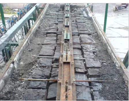
Creation of the physical model of the coal seam.
At the outlet, the composition of syngas was measured by stationary analyzers. The calorific value of syngas was calculated from the measured syngas composition. The underpressure at the outlet was controlled by an industrial fan and measured by a pressure gauge. The physical model of the underground coal bed was formed by blocks of Lignite-type coal from the Slovak mine (see Figure 2). Thermocouples of K-type were used to measure temperature in coal, overburden, underburden and gasification channels. To meet similarity conditions, the reactor was slightly inclined and sealed. Several experiments were performed on two ex-situ reactors (i.e., syngas generators 1 and 2). The comprehensive scheme of the experimental gasification equipment with two syngas generators is shown in Figure 3. These ex-situ reactors differ in dimensions. The bedding of coal corresponds to real coal seam with inclination. A monitoring system to monitor experiments was created in the SCADA/HMI application Promotic (see Figures 4 and 5). The monitoring system provided auxiliary algorithms for operating of the control system, plotting and archiving measured data from the gasification process to the database. The data recorded from experimental gasification during laboratory
erating of the control system, plotting and archiving measured data from the gasification process to the database. The data recorded from experimental gas-ification during laboratory gasgas-ification were also used in this paper to verify the proposed modeling method. The monitoring system was divided into screens, be-tween which the operator may switch.
The control of experimental UCG was ensured by PLC (B&R X20) that performed several cyclic tasks (i.e., data acquisition, data processing, process vari-ables stabilization via PI controllers, extremum seek-ing control, and optimal control based on gradient method). The PLC was connected with PC through RS232 and OPC protocol.
Information Technology and Control 2019/4/48 562
Figure 4
The main screen of the monitoring system
Figure 5
(a) Monitoring temperatures in the physical model, (b) Trends of various process variables.
(a) (b)
The control of experimental UCG was ensured by PLC (B&R X20) that performed several cyclic tasks (i.e., data acquisition, data processing, process variables stabilization via PI controllers, extremum
seeking control, and optimal control based on gradient method). The PLC was connected with PC through RS232 and OPC protocol.
The proposed monitoring system for Figure 5
(a) Monitoring temperatures in the physical model, (b) Trends of various process variables.
(a) (b)
The control of experimental UCG was ensured by PLC (B&R X20) that performed several cyclic tasks (i.e., data acquisition, data processing, process variables stabilization via PI controllers, extremum
seeking control, and optimal control based on gradient method). The PLC was connected with PC through RS232 and OPC protocol.
The proposed monitoring system for
Figure 5
(a) Monitoring temperatures in the physical model, (b) Trends of various process variables.
(a) (b)
The control of experimental UCG was ensured by PLC (B&R X20) that performed several cyclic tasks (i.e., data acquisition, data processing, process variables stabilization via PI controllers, extremum
seeking control, and optimal control based on gradient method). The PLC was connected with PC through RS232 and OPC protocol.
The proposed monitoring system for
Figure 5
(a) Monitoring temperatures in the physical model, (b) Trends of various process variables
563 Information Technology and Control 2019/4/48
3. UCG Modeling Based on MARS
Currently, various methods for nonlinear system modeling are applied in research, e.g., Neural Net-works (NN), Nonlinear Finite Impulse Response (NFIR), Nonlinear AutoRegressive with eXogenous inputs (NARX), Nonlinear AutoRegressive Moving Average with eXogenous input (NARMAX), Non-linear Output Error (NOE) model, and NonNon-linear Box-Jenkins (NBJ) model. This section explains the background of the black-box method called Multivar-iate Adaptive Regression Splines (MARS) that can model nonlinearities in the UCG process. The model can be created from offline UCG observations and tar-gets. The goal is to find the dependency of variables yi on one or more independent variables ui. The follow-ing regression sample is considered:experimental gasification equipment is able to monitor and record various process variables, e.g., injected air volume flow, injected air overpressure, injected oxygen volume flow, injected oxygen overpressure, exhausting underpressure, syngas temperature, concentrations of O2, CO2, H2, CO,
CH4 in syngas, calorific value of syngas, syngas
volume flow, temperatures of overburden layers, temperatures inside gasifier (i.e., in oxidizing, reducing, and pyrolyzing zone), and temperatures of underburden layers.
3. UCG Modeling Based on MARS
Currently, various methods for nonlinear system modeling are applied in research, e.g., Neural Networks (NN), Nonlinear Finite Impulse Response (NFIR), Nonlinear AutoRegressive with eXogenous inputs (NARX), Nonlinear AutoRegressive Moving Average with eXogenous input (NARMAX), Nonlinear Output Error (NOE) model, and Nonlinear Box-Jenkins (NBJ) model. This section explains the background of the black-box method called Multivariate Adaptive Regression Splines (MARS) that can model nonlinearities in the UCG process. The model can be created from offline UCG observations and targets. The goal is to find the dependency of variables yi on one or more independent variables ui. The following regression sample is considered:
,
1
1, , ,
1,N N
i i i i n i i i
D u y u u y (1)
where ui∈ℝn represents the i-th vector of the independent variables; yi∈ℝ, (i = 1, …, N) is the
dependent variable, i.e., target; n represents the number of independent variables, and N
represents the number of samples, i.e., the total number of (ui, yi) pairs. These variables represent
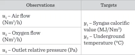
manipulated variables and measured output in UCG. In experimental UCG, three manipulation variables (i.e., input observations) and two controlled variables (i.e., targets) have been specified (see Table 1).
Table 1
Selected observations and targets in UCG
OObbsseerrvvaattiioonnss TTaarrggeettss u1 – Air flow
(Nm3/h) y1 – Syngas calorific
value (MJ/Nm3) y2 – Underground temperature (°C)
u2 – Oxygen flow (Nm3/h)
u3 – Outlet relative pressure (Pa)
The MARS method was firstly introduced in [18] and represents a non-parametric regression technique that can automatically model nonlinearities and interactions between process variables. If the MARS technique of regression analysis on time series is used, the autoregressive model can be obtained. Many works have been published that discussed the MARS method (e.g., [14, 19, 51]).
In order to create the MARS model, the training data vectors, i.e., the inputs (observations) and outputs (targets) are needed. Training data are split into several splines on an equivalent interval basis. The data are in every spline split into many subgroups, and several knots are created that can be placed between different input variables or different intervals in the same input variable to separating subgroups [14]. To verify the performance of the model being created, the model is verified on the test data. In MARS, the regression function called basis function (BF) is approximated by smoothing splines for a general representation of data in each subgroup. Between any two knots, the model can characterize the data either globally or by using linear regression. The BF is unique between any two knots and is shifted to another BF at each knot. Two BFs in two adjacent domains of data intersect at the knot to make model outputs continuous. MARS creates a curved regression line to fit the data from subgroup to subgroup and from one spline to another spline. For evading over-fitting and over-regressing, the shortest distance between two neighboring knots is predetermined to prevent too few data in a subgroup [18]. In the MARS method, the goal is to find the dependency of variables yi on one or more independent
variables ui. The relationship between yi and ui (i
= 1, …, N) can be represented as:
1, 2, , n
( ) ,i i i i i
y f u u u f u (2)
where 𝑓𝑓 is an unknown function, and ε is an error
(ε~N(0,σ2)). The single-valued deterministic
function f captures the joint predictive relationship of yi on (ui1,ui2,...,uin). The additive
stochastic component ε usually reflects the dependence of yi on values other than
(ui1,ui2,...,uin), that are neither controlled nor
observed.
In the one-dimensional case, splines are expressed in terms of piecewise linear basis functions, (u-t)+ and (t-u)+ with the node in t. The "+" means a positive part. These functions are (1)
where ui∈ℝn represents the i-th vector of the inde-pendent variables; yi∈ℝ, (i = 1, …, N) is the dependent variable, i.e., target; n represents the number of inde-pendent variables, and N represents the number of samples, i.e., the total number of (ui, yi) pairs. These variables represent manipulated variables and mea-sured output in UCG. In experimental UCG, three ma-nipulation variables (i.e., input observations) and two controlled variables (i.e., targets) have been specified (see Table 1).
Table 1
Selected observations and targets in UCG
Observations Targets
u1 – Air flow
(Nm3/h) y
1 – Syngas calorific value (MJ/Nm3)
y2 – Underground temperature (°C)
u2 – Oxygen flow (Nm3/h)
u3 – Outlet relative pressure (Pa)
The MARS method was firstly introduced in [18] and represents a non-parametric regression technique that can automatically model nonlinearities and in-teractions between process variables. If the MARS technique of regression analysis on time series is used, the autoregressive model can be obtained. Many works have been published that discussed the MARS method (e.g., [14, 19, 51]).
In order to create the MARS model, the training data vectors, i.e., the inputs (observations) and outputs (targets) are needed. Training data are split into sever-al splines on an equivsever-alent intervsever-al basis. The data are in every spline split into many subgroups, and several knots are created that can be placed between differ-ent input variables or differdiffer-ent intervals in the same input variable to separating subgroups [14]. To verify the performance of the model being created, the mod-el is verified on the test data. In MARS, the regression function called basis function (BF) is approximated by smoothing splines for a general representation of data in each subgroup. Between any two knots, the model can characterize the data either globally or by using linear regression. The BF is unique between any two knots and is shifted to another BF at each knot. Two BFs in two adjacent domains of data intersect at the knot to make model outputs continuous. MARS creates a curved regression line to fit the data from subgroup to subgroup and from one spline to anoth-er spline. For evading ovanoth-er-fitting and ovanoth-er-regress- over-regress-ing, the shortest distance between two neighboring knots is predetermined to prevent too few data in a subgroup [18]. In the MARS method, the goal is to find the dependency of variables yi on one or more inde-pendent variables ui. The relationship between yi and ui (i = 1, …, N) can be represented as:
experimental gasification equipment is able to monitor and record various process variables, e.g., injected air volume flow, injected air overpressure, injected oxygen volume flow, injected oxygen overpressure, exhausting underpressure, syngas temperature, concentrations of O2, CO2, H2, CO,
CH4 in syngas, calorific value of syngas, syngas
volume flow, temperatures of overburden layers, temperatures inside gasifier (i.e., in oxidizing, reducing, and pyrolyzing zone), and temperatures of underburden layers.
3. UCG Modeling Based on MARS
Currently, various methods for nonlinear system modeling are applied in research, e.g., Neural Networks (NN), Nonlinear Finite Impulse Response (NFIR), Nonlinear AutoRegressive with eXogenous inputs (NARX), Nonlinear AutoRegressive Moving Average with eXogenous input (NARMAX), Nonlinear Output Error (NOE) model, and Nonlinear Box-Jenkins (NBJ) model. This section explains the background of the black-box method called Multivariate Adaptive Regression Splines (MARS) that can model nonlinearities in the UCG process. The model can be created from offline UCG observations and targets. The goal is to find the dependency of variables yi on one or more independent variables ui. The following regression sample is considered:
,
1
1, , ,
1,N N
i i i i n i i i
D u y u u y (1)
where ui∈ℝn represents the i-th vector of the
independent variables; yi∈ℝ, (i = 1, …, N) is the
dependent variable, i.e., target; n represents the number of independent variables, and N represents the number of samples, i.e., the total number of (ui, yi) pairs. These variables represent
manipulated variables and measured output in UCG. In experimental UCG, three manipulation variables (i.e., input observations) and two controlled variables (i.e., targets) have been specified (see Table 1).
Table 1
Selected observations and targets in UCG
OObbsseerrvvaattiioonnss TTaarrggeettss u1 – Air flow
(Nm3/h) y1 – Syngas calorific
value (MJ/Nm3) y2– Underground
temperature (°C)
u2– Oxygen flow
(Nm3/h)
u3– Outlet relative pressure
(Pa)
The MARS method was firstly introduced in [18] and represents a non-parametric regression technique that can automatically model nonlinearities and interactions between process variables. If the MARS technique of regression analysis on time series is used, the autoregressive model can be obtained. Many works have been published that discussed the MARS method (e.g., [14, 19, 51]).
In order to create the MARS model, the training data vectors, i.e., the inputs (observations) and outputs (targets) are needed. Training data are split into several splines on an equivalent interval basis. The data are in every spline split into many subgroups, and several knots are created that can be placed between different input variables or different intervals in the same input variable to separating subgroups [14]. To verify the performance of the model being created, the model is verified on the test data. In MARS, the regression function called basis function (BF) is approximated by smoothing splines for a general representation of data in each subgroup. Between any two knots, the model can characterize the data either globally or by using linear regression. The BF is unique between any two knots and is shifted to another BF at each knot. Two BFs in two adjacent domains of data intersect at the knot to make model outputs continuous. MARS creates a curved regression line to fit the data from subgroup to subgroup and from one spline to another spline. For evading over-fitting and over-regressing, the shortest distance between two neighboring knots is predetermined to prevent too few data in a subgroup [18]. In the MARS method, the goal is to find the dependency of variables yi on one or more independent
variables ui. The relationship between yi and ui (i
= 1, …, N) can be represented as:
1, 2, , n
( ) ,i i i i i
y f u u u f u (2)
where 𝑓𝑓 is an unknown function, and ε is an error
(ε~N(0,σ2)). The single-valued deterministic function f captures the joint predictive relationship of yi on (ui1,ui2,...,uin). The additive
stochastic component ε usually reflects the dependence of yi on values other than
(ui1,ui2,...,uin), that are neither controlled nor
observed.
In the one-dimensional case, splines are expressed in terms of piecewise linear basis functions, (u-t)+ and (t-u)+ with the node in t. The "+" means a positive part. These functions are
(2) where f is an unknown function, and ε is an error (ε~N(0,σ2)). The single-valued deterministic function f captures the joint predictive relationship of yi on (ui1,ui2,...,uin). The additive stochastic component ε usu-ally reflects the dependence of yi on values other than (ui1,ui2,...,uin), that are neither controlled nor observed. In the one-dimensional case, splines are expressed in terms of piecewise linear basis functions, (u-t)+ and (t-u)+ with the node in t. The “+” means a positive part. These functions are truncated linear functions, for u∈ℝ:
truncated linear functions, for u∈ℝ:
, If ,
( ) and
0, otherwise
u t u t
u t
, If , ( )
0, otherwise.
t u u t
t u
(3)
Each function (i.e., (u-t)+ and (t-u)+) is piecewise
linear, with a knot at the value t. They are marked as linear splines. These two functions are named as a reflected pair. In the multidimensional case, the idea is to form reflected pairs for each input component uj of the vector u=(u1,...,uj,...,un)T with
knots at each observed value uij of that input
(i=1,2,...,N; j=1,2,...,n). Thus, a set of constructed basis functions can be expressed as follows:
1 2
( ) , ( ) | , , , ,
1, 2, , .
j j j j j
N
C u t t u t u u u
j n
(4)
If all input data are different, then in the set of 2Nn basis functions, each of them depends on only one variable uj. For example, B(u)=(uj-t)+ is regarded as
a function over the entire input space ℝn. Basis
functions used for approximation are as follows:
,
,
1 ,
m
K
v k m km
m k m
k
B s u t
u (5)
where Km represents the total number of truncated
linear functions in the m-th basis function, u(v(k,m)) is
the component of the vector u, related to the k-th truncated linear function in the m-th basic function, tkm is the corresponding node, and sk,m∈{±1}. Parameter Km is by user-defined degree order of
the interaction term and sk,m represents the
direction of the univariate term, which could be positive or negative.
The model-building strategy is like a forward stepwise linear regression, but instead of using the original inputs, it is allowed to use functions from the set C of their products. Therefore, the MARS model can be expressed by the following equation
0
1
ˆ
Mm m
,
m
y f
c
c B
u
u
(6)where y is the output variable, u represents the vector of input variables, M is the number of basis functions in the model (i.e., number of spline functions), c0 is the coefficient of the constant basis
function B0, and the sum is over the basis
functions Bm produced by an algorithm that
implements the forward stepwise part of the MARS strategy by incorporating the modification to recursive partitioning. The coefficients 𝑐𝑐� are estimated by minimizing the residual sum-of-squares. Bm(u) is the m-th function in C, or a
product of two or more such functions.
The most important thing in this model is the choice of the basis functions. In the beginning, the model contains a single function B0(u)=1 and all
functions from the set C are possible candidates for inclusion in the model. As in linear regression, setting Bm, the coefficients cm can be found by the
method of least squares. Another subroutine of MARS performs the backward deletion strategy wherein each iteration causes one unnecessary (i.e., redundant) basis function to be deleted. A function whose removal either mostly improves the fit or at least degrades it will be deleted. However, the constant basis function B1(u)=1 is
never removed.
4. Model Predictive Control
Nowadays, various methods of technological process control are being developed, e.g., [42, 44]. The MPC controller is conceived as multidimensional, i.e., it works in a coordinated manner with a higher number of manipulated variables (MVs) and controlled variables, i.e., measured outputs (MOs) what is typical in MIMO or MISO systems. All limitations on permitted ranges of values and rate of change of regulated and action variables are already respected when calculating action interventions and not additionally. At any time of sampling, the following must be available: dynamic control system model, including restrictive conditions; current and past values of controlled variables; previous values of manipulated variables; known or expected course of desired values of controlled variables within the assumed horizon of prediction N. For comparison, MPC responds to the predicted future value of control errors, PID only to current and past values. At each moment of sampling, the optimization task is solved, and the calculation of manipulated variables is performed within the considered control horizon Nu. The control sequence has the following form:
k k| , k 1| , k
k 2| , k
u u u
, k Nu 1| .k
u (7)
It is assumed that u(k+p│k)=u(k+Nu-1│k) for p≥Nu.
(3)
Information Technology and Control 2019/4/48 564
linear splines. These two functions are named as a reflected pair. In the multidimensional case, the idea is to form reflected pairs for each input component uj of the vector u=(u1,...,uj,...,un)T with knots at each observed value uij of that input (i=1,2,...,N; j=1,2,...,n). Thus, a set of constructed basis functions can be ex-pressed as follows:
1 2( ) , ( ) | , , , ,
1, 2, , .
j j j j j
N
C u t t u t u u u
j n
If all input data are different, then in the set of (4)
If all input data are different, then in the set of 2Nn basis functions, each of them depends on only one variable uj. For example, B(u)=(uj-t)
+ is regarded as a function over the entire input space ℝn. Basis func-tions used for approximation are as follows:
truncated linear functions, for u∈ℝ:
, If ,
( ) and
0, otherwise
u t u t
u t
, If , ( )
0, otherwise.
t u u t
t u
(3)
Each function (i.e., (u-t)+ and (t-u)+) is piecewise linear, with a knot at the value t. They are marked as linear splines. These two functions are named as a reflected pair. In the multidimensional case, the idea is to form reflected pairs for each input component uj of the vector u=(u1,...,uj,...,un)T with
knots at each observed value uij of that input
(i=1,2,...,N; j=1,2,...,n). Thus, a set of constructed basis functions can be expressed as follows:
1 2
( ) , ( ) | , , , , 1, 2, , .
j j j j j
N
C u t t u t u u u
j n
(4)
If all input data are different, then in the set of 2Nn
basis functions, each of them depends on only one variable uj. For example, B(u)=(uj-t)+ is regarded as
a function over the entire input space ℝn. Basis
functions used for approximation are as follows:
,
, 1 , m Kv k m km
m k m
k
B s u t
u (5)
where Km represents the total number of truncated
linear functions in the m-th basis function, u(v(k,m)) is
the component of the vector u, related to the k-th truncated linear function in the m-th basic function,
tkm is the corresponding node, and sk,m∈{±1}.
Parameter Km is by user-defined degree order of
the interaction term and sk,m represents the
direction of the univariate term, which could be positive or negative.
The model-building strategy is like a forward stepwise linear regression, but instead of using the original inputs, it is allowed to use functions from the set C of their products. Therefore, the MARS model can be expressed by the following equation
0
1
ˆ
Mm m
,
m
y f
c
c B
u
u
(6)where y is the output variable, u represents the vector of input variables, M is the number of basis functions in the model (i.e., number of spline functions), c0 is the coefficient of the constant basis
function B0, and the sum is over the basis
functions Bm produced by an algorithm that
implements the forward stepwise part of the MARS strategy by incorporating the modification to recursive partitioning. The coefficients 𝑐𝑐� are
estimated by minimizing the residual sum-of-squares. Bm(u) is the m-th function in C, or a
product of two or more such functions.
The most important thing in this model is the choice of the basis functions. In the beginning, the model contains a single function B0(u)=1 and all functions from the set C are possible candidates for inclusion in the model. As in linear regression, setting Bm, the coefficients cm can be found by the
method of least squares. Another subroutine of MARS performs the backward deletion strategy wherein each iteration causes one unnecessary (i.e., redundant) basis function to be deleted. A function whose removal either mostly improves the fit or at least degrades it will be deleted. However, the constant basis function B1(u)=1 is never removed.
4. Model Predictive Control
Nowadays, various methods of technological process control are being developed, e.g., [42, 44]. The MPC controller is conceived as multidimensional, i.e., it works in a coordinated manner with a higher number of manipulated variables (MVs) and controlled variables, i.e., measured outputs (MOs) what is typical in MIMO or MISO systems. All limitations on permitted ranges of values and rate of change of regulated and action variables are already respected when calculating action interventions and not additionally. At any time of sampling, the following must be available: dynamic control system model, including restrictive conditions; current and past values of controlled variables; previous values of manipulated variables; known or expected course of desired values of controlled variables within the assumed horizon of prediction N. For comparison, MPC responds to the predicted future value of control errors, PID only to current and past values. At each moment of sampling, the optimization task is solved, and the calculation of manipulated variables is performed within the considered control horizon
Nu. The control sequence has the following form:
k k| , k 1| , k
k 2| , k
u u u
, k Nu 1| .k
u (7)
It is assumed that u(k+p│k)=u(k+Nu-1│k) for p≥Nu.
(5)
where Km represents the total number of truncated linear functions in the m-th basis function, u(v(k,m)) is the component of the vector u, related to the k-th truncated linear function in the m-th basic function, tkm is the corresponding node, and s
k,m∈{±1}. Parame-ter Km is by user-defined degree order of the interac-tion term and sk,m represents the direction of the uni-variate term, which could be positive or negative. The model-building strategy is like a forward step-wise linear regression, but instead of using the origi-nal inputs, it is allowed to use functions from the set C of their products. Therefore, the MARS model can be expressed by the following equation
truncated linear functions, for u∈ℝ:
, If ,
( ) and
0, otherwise
u t u t
u t
, If ,
( )
0, otherwise.
t u u t
t u
(3)
Each function (i.e., (u-t)+ and (t-u)+) is piecewise
linear, with a knot at the value t. They are marked as linear splines. These two functions are named as a reflected pair. In the multidimensional case, the idea is to form reflected pairs for each input component uj of the vector u=(u1,...,uj,...,un)T with
knots at each observed value uij of that input
(i=1,2,...,N; j=1,2,...,n). Thus, a set of constructed basis functions can be expressed as follows:
1 2
( ) , ( ) | , , , ,
1, 2, , .
j j j j j
N
C u t t u t u u u
j n
(4)
If all input data are different, then in the set of 2Nn basis functions, each of them depends on only one variable uj. For example, B(u)=(uj-t)+ is regarded as
a function over the entire input space ℝn. Basis
functions used for approximation are as follows:
,
,
1 ,
m
K
v k m km
m k m
k
B s u t
u (5)
where Km represents the total number of truncated
linear functions in the m-th basis function, u(v(k,m)) is
the component of the vector u, related to the k-th truncated linear function in the m-th basic function,
tkm is the corresponding node, and sk,m∈{±1}. Parameter Km is by user-defined degree order of
the interaction term and sk,m represents the
direction of the univariate term, which could be positive or negative.
The model-building strategy is like a forward stepwise linear regression, but instead of using the original inputs, it is allowed to use functions from the set C of their products. Therefore, the MARS model can be expressed by the following equation
0
1
ˆ
Mm m
,
m
y f
c
c B
u
u
(6)where y is the output variable, u represents the vector of input variables, M is the number of basis functions in the model (i.e., number of spline functions), c0 is the coefficient of the constant basis
function B0, and the sum is over the basis
functions Bm produced by an algorithm that
implements the forward stepwise part of the MARS strategy by incorporating the modification to recursive partitioning. The coefficients 𝑐𝑐� are
estimated by minimizing the residual sum-of-squares. Bm(u) is the m-th function in C, or a
product of two or more such functions.
The most important thing in this model is the choice of the basis functions. In the beginning, the model contains a single function B0(u)=1 and all
functions from the set C are possible candidates for inclusion in the model. As in linear regression, setting Bm, the coefficients cm can be found by the
method of least squares. Another subroutine of MARS performs the backward deletion strategy wherein each iteration causes one unnecessary (i.e., redundant) basis function to be deleted. A function whose removal either mostly improves the fit or at least degrades it will be deleted. However, the constant basis function B1(u)=1 is
never removed.
4. Model Predictive Control
Nowadays, various methods of technological process control are being developed, e.g., [42, 44]. The MPC controller is conceived as multidimensional, i.e., it works in a coordinated manner with a higher number of manipulated variables (MVs) and controlled variables, i.e., measured outputs (MOs) what is typical in MIMO or MISO systems. All limitations on permitted ranges of values and rate of change of regulated and action variables are already respected when calculating action interventions and not additionally. At any time of sampling, the following must be available: dynamic control system model, including restrictive conditions; current and past values of controlled variables; previous values of manipulated variables; known or expected course of desired values of controlled variables within the assumed horizon of prediction N. For comparison, MPC responds to the predicted future value of control errors, PID only to current and past values. At each moment of sampling, the optimization task is solved, and the calculation of manipulated variables is performed within the considered control horizon Nu. The control sequence has the following form:
k k| , k 1| , k
k 2| , k
u u u
, k Nu 1| .k
u (7)
It is assumed that u(k+p│k)=u(k+Nu-1│k) for p≥Nu.
(6)
where y is the output variable, u represents the vector of input variables, M is the number of basis functions in the model (i.e., number of spline functions), c0 is the coefficient of the constant basis function B0, and the sum is over the basis functions Bm produced by an al-gorithm that implements the forward stepwise part of the MARS strategy by incorporating the modification to recursive partitioning. The coefficients cm are es-timated by minimizing the residual sum-of-squares. Bm(u) is the m-th function in C, or a product of two or more such functions.
The most important thing in this model is the choice of the basis functions. In the beginning, the model contains a single function B0(u)=1 and all functions from the set C are possible candidates for inclusion in the model. As in linear regression, setting Bm, the coefficients cm can be found by the method of least squares. Another subroutine of MARS performs the backward deletion strategy wherein each iteration causes one unnecessary (i.e., redundant) basis func-tion to be deleted. A funcfunc-tion whose removal either mostly improves the fit or at least degrades it will be deleted. However, the constant basis function B1(u)=1 is never removed.
4. Model Predictive Control
Nowadays, various methods of technological pro-cess control are being developed, e.g., [42, 44]. The MPC controller is conceived as multidimensional, i.e., it works in a coordinated manner with a higher number of manipulated variables (MVs) and con-trolled variables, i.e., measured outputs (MOs) what is typical in MIMO or MISO systems. All limitations on permitted ranges of values and rate of change of regulated and action variables are already respected when calculating action interventions and not addi-tionally. At any time of sampling, the following must be available: dynamic control system model, includ-ing restrictive conditions; current and past values of controlled variables; previous values of manipulated variables; known or expected course of desired values of controlled variables within the assumed horizon of prediction N. For comparison, MPC responds to the predicted future value of control errors, PID only to current and past values. At each moment of sampling, the optimization task is solved, and the calculation of manipulated variables is performed within the con-sidered control horizon Nu. The control sequence has the following form:
truncated linear functions, for u∈ℝ:
, If , ( ) and
0, otherwise
u t u t
u t
, If , (t u) t u0, otherwise.u t
(3)
Each function (i.e., (u-t)+ and (t-u)+) is piecewise
linear, with a knot at the value t. They are marked as linear splines. These two functions are named as a reflected pair. In the multidimensional case, the idea is to form reflected pairs for each input component uj of the vector u=(u1,...,uj,...,un)T with
knots at each observed value uij of that input (i=1,2,...,N; j=1,2,...,n). Thus, a set of constructed basis functions can be expressed as follows:
1 2
( ) , ( ) | , , , , 1, 2, , .
j j j j j
N
C u t t u t u u u
j n
(4)
If all input data are different, then in the set of 2Nn
basis functions, each of them depends on only one variable uj. For example, B(u)=(uj-t)+ is regarded as
a function over the entire input space ℝn. Basis
functions used for approximation are as follows:
,
, 1 , m Kv k m km
m k m
k
B s u t
u (5)
where Km represents the total number of truncated
linear functions in the m-th basis function, u(v(k,m)) is
the component of the vector u, related to the k-th truncated linear function in the m-th basic function, tkm is the corresponding node, and sk,m∈{±1}.
Parameter Km is by user-defined degree order of
the interaction term and sk,m represents the
direction of the univariate term, which could be positive or negative.
The model-building strategy is like a forward stepwise linear regression, but instead of using the original inputs, it is allowed to use functions from the set C of their products. Therefore, the MARS model can be expressed by the following equation
0
1
ˆ
Mm m
,
m
y f
c
c B
u
u
(6)where y is the output variable, u represents the vector of input variables, M is the number of basis functions in the model (i.e., number of spline functions), c0 is the coefficient of the constant basis
function B0, and the sum is over the basis
functions Bm produced by an algorithm that
implements the forward stepwise part of the MARS strategy by incorporating the modification to recursive partitioning. The coefficients 𝑐𝑐� are
estimated by minimizing the residual sum-of-squares. Bm(u) is the m-th function in C, or a
product of two or more such functions.
The most important thing in this model is the choice of the basis functions. In the beginning, the model contains a single function B0(u)=1 and all
functions from the set C are possible candidates for inclusion in the model. As in linear regression, setting Bm, the coefficients cm can be found by the
method of least squares. Another subroutine of MARS performs the backward deletion strategy wherein each iteration causes one unnecessary (i.e., redundant) basis function to be deleted. A function whose removal either mostly improves the fit or at least degrades it will be deleted. However, the constant basis function B1(u)=1 is
never removed.
4. Model Predictive Control
Nowadays, various methods of technological process control are being developed, e.g., [42, 44]. The MPC controller is conceived as multidimensional, i.e., it works in a coordinated manner with a higher number of manipulated variables (MVs) and controlled variables, i.e., measured outputs (MOs) what is typical in MIMO or MISO systems. All limitations on permitted ranges of values and rate of change of regulated and action variables are already respected when calculating action interventions and not additionally. At any time of sampling, the following must be available: dynamic control system model, including restrictive conditions; current and past values of controlled variables; previous values of manipulated variables; known or expected course of desired values of controlled variables within the assumed horizon of prediction N. For comparison, MPC responds to the predicted future value of control errors, PID only to current and past values. At each moment of sampling, the optimization task is solved, and the calculation of manipulated variables is performed within the considered control horizon
Nu. The control sequence has the following form:
k k| , k 1| , k
k 2| , k
u u u
, k Nu 1| .k
u (7)
It is assumed that u(k+p│k)=u(k+Nu-1│k) for p≥Nu. (7)


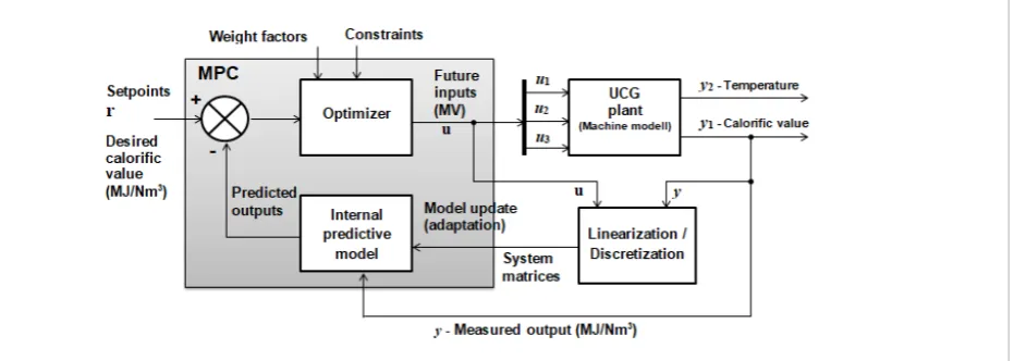
![Figure 11 Matlab-Simulink block scheme for adaptive MPC simulation (modified after [6])](https://thumb-us.123doks.com/thumbv2/123dok_us/8763345.1753159/16.595.72.532.109.329/figure-matlab-simulink-block-scheme-adaptive-simulation-modified.webp)