Detecting coherent patterns in a flume by using PIV and IR imaging techniques

Detecting coherent patterns in a flume by using PIV and IR

imaging techniques

Roi Gurka, Alex Liberzon, Gad Hetsroni

Abstract We investigated the flow field in a turbulent boundary layer in a flume, by using Particle Image Ve-locimetry (PIV) and Hot-Foil Infrared Imaging (HFIRI) techniques. Coherent patterns in the flow were identified and characterized by using instantaneous velocity and temperature fields. The velocity fields in the streamwise– spanwise plane were measured in parallel to the temper-ature distribution of the flume bottom. The identified patterns are represented by means of their spatial char-acteristics – a non-dimensional spatial separation between streamwise patterns,k+.

1

Introduction

Wall bounded turbulent flows have been discussed exten-sively in the literature, in particular the coherent structures in this region (see for example Panton 1997). The coherent structures account for over 80% of the energy in the tur-bulent fluctuations, during the bursting process (Kim et al. 1971), related to the transport of the fluid from the low-speed regions to the main stream, and sweeping of fluid from the outer region toward the wall (Robinson 1991). High- and low-speed streaks are the most well recognized coherent structures, originally discovered by Kline et al. (1967), by using hydrogen bubble flow visualization. Since then, a variety of experimental techniques have been utilized for investigation of low-speed streaks, including bubble or particle tracer visualization (among others: Rashidi and Banerjee 1990; Smith and Metzler 1983), hot-wire ane-mometry (e.g., Nakagawa and Nezu 1981), and particle

image velocimetry (PIV) (Adrian 1991). A list of the experimental investigation of the coherent patterns in the near-wall region is far too long to review.

A comprehensive study of the heat transfer, in addition to the momentum transfer in the near-wall region, relies on the quantitative information about thermal and velocity fields. Unfortunately, most of the available non-intrusive measurement techniques, such as laser-Doppler veloci-metry (LDV), planar laser induced florescence (PLIF) and PIV, have limited accuracy at small non-dimensional dis-tances from the wall. The direct evidence of the fluid-wall interactions can be visualized by using the heated-thin-foil technique, which has been successfully applied to a variety of convective heat transfer measurements (De Luca et al. 1990; Carlomagno 1997), and implemented for turbulent boundary layer research (Hetsroni and Rozenblit 1994). The idea is based on the assumption, that the ordered thermal patterns show fluctuations of the temperature field due to the exchange of the low- and high-momentum fluid between the near-wall and the outer regions of the boundary layer, respectively.

Hetsroni et al. (2001) and Kowalewski et al. (2003) used this assumption as a basis for the indirect measurement of the convective velocity through IR imaging of the hot-foil and tracking of the displacement of the thermal patterns. It was shown by Iritani et al. (1983) and Kim (1989), that the scalar fields in the wall region are highly correlated with the streamwise velocity. In the present study we extended the experimental technique (Hetsroni et al. 2001;

Kowalewski et al. 2003) toward the direct measurement of the velocity field in addition to the thermal patterns measurements by using the HFIRI method. The combined PIV and HFIRI measurement technique which allows for the instantaneous correlated analysis of the momentum and heat transfer in the near-wall region is presented.

In Sect. 2 we present the experimental setup, experi-mental conditions and the optical configuration of PIV and HFIRI, followed by the description of the combined technique in Sect. 3. The preliminary results and discus-sions are provided in Sect. 4 and concluded by the sum-mary in Sect. 5.

2

Experimental setup 2.1

Infrastructure

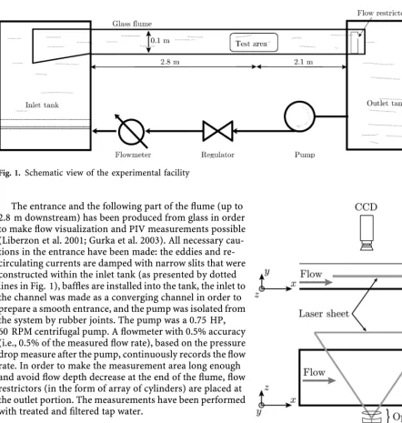
The experiments were conducted in a horizontal flume of 4.9·0.32·0.1 m as shown in Fig. 1.

230

Received: 10 September 2003 / Accepted: 26 February 2004 Published online: 15 April 2004

Springer-Verlag 2004

R. Gurka, A. Liberzon, G. Hetsroni (&)

Multiphase Flow Laboratory, Mechanical Engineering Department, Technion-IIT, 32000 Haifa, Israel

E-mail: [email protected] http://multiphaselab.technion.ac.il

Present address: R. Gurka

Department of Mechanical Engineering, Johns Hopkins University, Baltimore, MD USA

Present address: A. Liberzon

Institute of Hydromechanics and Water Resources Management, ETH Zu¨rich, Switzerland

The entrance and the following part of the flume (up to 2.8 m downstream) has been produced from glass in order to make flow visualization and PIV measurements possible (Liberzon et al. 2001; Gurka et al. 2003). All necessary cau-tions in the entrance have been made: the eddies and re-circulating currents are damped with narrow slits that were constructed within the inlet tank (as presented by dotted lines in Fig. 1), baffles are installed into the tank, the inlet to the channel was made as a converging channel in order to prepare a smooth entrance, and the pump was isolated from the system by rubber joints. The pump was a 0.75 HP, 60 RPM centrifugal pump. A flowmeter with 0.5% accuracy (i.e., 0.5% of the measured flow rate), based on the pressure drop measure after the pump, continuously records the flow rate. In order to make the measurement area long enough and avoid flow depth decrease at the end of the flume, flow restrictors (in the form of array of cylinders) are placed at the outlet portion. The measurements have been performed with treated and filtered tap water.

2.2

Particle Image Velocimetry (PIV) setup

The PIV system, schematically shown in Fig. 2 was com-posed of a double Nd:YAG laser (170 mJ/pulse, 15 Hz) and a 1K·1K, 30 frames-per-second (fps), 8-bit CCD camera. Hollow glass spherical particles with an average diameter of 11lm were used for seeding. The calibration procedure and the PIV cross-correlation analysis were performed by using Insight 3.2 software (TSI). We used 64·64 pixels interro-gation areas, with a 100lm/pixel ratio and 50% overlap-ping. The analysis produced about 1000 vectors in each given field of view, filtered by using standard median and global outlier filters. On average, about 5% of the erroneous vectors were removed during the post-processing analysis (Nogueira et al. 1997). The statistical analysis was based on 200 image pairs for each experimental case, resulting in 200 velocity vector fields in the streamwise-spanwise plane. The standard error analysis, based on the assumption that the velocity data has a normal distribution, shows that for the mean velocity value of 0.2 m/s, for a sample size of 100, and a probability of 95%, the uncertainty level is estimated to be lower than ±0.005 m/s.

We present the results of the measurements in the streamwise–spanwise (x–z) plane (Fig. 2). The coordinates

x,y,zshould be defined relatively to the coordinate system with the origin at the left lower corner of the inlet of the flume. The region of interest was located at a distance 2.8 m from the inlet. The experiments were done at three different flow rates, listed in Table 1.

2.3

Hot-Foil Infrared Imaging (HFIRI) setup

An infrared technique was used to investigate the tem-perature field on the bottom of the flume. This method is based on measurement of the local temperatures of the surface of a heated film, by means of infrared thermog-raphy (Hetsroni et al. 1996; Hetsroni et al. 1997). The HFIRI (Fig. 3) measures the local temperatures on the surface by means of a remote detector of electromagnetic radiation. In order to measure the temperature distribu-tion, part of the flume bottom has to be heated slightly.

Fig. 1. Schematic view of the experimental facility

Fig. 2. Schematic view of the PIV setup

The constantan heater was made of a foil 0.33 m long, 0.2 m wide and 50lm thick. The foil was attached to the insulated frame, with dimensions of 0.3·0.15 m, by means of contact adhesive and was coated, on the air side, by black mat paint of about 20lm thickness. The window with the foil was accurately installed at the bottom of the flume. As a result, the unpainted side of the foil functioned as the bottom wall of the flume. Constant heat flux was supplied from a DC power supply up to 1 A.

The Inframetrics model 740 infrared imaging radiom-eter was used for the investigation of the temperature distribution on the foil surface. The IR radiometer consists of a scanner and a control/electronics unit. A Mercury/ Cadmium/Telluride detector is cooled by an integrated cooler to 77 K for maximum thermal sensitivity and high spatial resolution. The temperature range of the IR scan-ner, reported by the manufacturer, is)20C to 1400C, with a minimum detectable temperature difference of 0.1 K at 30C. Through the calibration, the thermal imaging radiometer is very accurate in a narrow temper-ature range giving a typical noise equivalent tempertemper-ature difference only, which is less than 0.2 K (with image average less than 0.05 K). For all of the performance characteristics mentioned above, it was assumed that the surface of the heater behaves almost like a black body (e0.96).

The IR Radiometer was situated under the foil at a distance of about 0.5 m. Hetsroni and Rozenblit (1994) demonstrated that there is an insignificant temperature difference (0.1 K) between the temperatures of the top and bottom of the thin heater. The calibration of the IR radiometer was checked in the flume with a precision mercury thermometer placed in the water. The accuracy of the IR radiometer, according to the manufacturer data equals to ±2%. The heat flux (DC power) was determined with accuracy of 0.5%. Accordingly, the errors in mea-surements of the wall temperature did not exceed ±2% (Hetsroni et al. 1996).

3

Combination of the PIV and HFIRI systems

The PIV system, shown in Fig. 2 and the HFIRI system, presented in Fig. 3, were combined in this study as is demonstrated in Fig. 4, in order to obtain the coupled velocity-temperature information. The combination of PIV and HFIRI techniques provides instantaneous measure-ments of the thermal and the velocity fields in the turbu-lent boundary layer. The need to characterize the flow field very close to the wall demands a measurement technique which will provide data aty=0. Optical methods, based on laser illumination, are limited to measure at these resolu-tions, due to optical limitations. In particular, the PIV method, which is based on the diffractive light from the tracer particles, requires illuminating the flow field, which causes strong reflections from the wall. In addition, the usage of seeded tracer particles inherently limits the ability to measure the velocity at the proximity of the wall (y0). The advantage of the HFIRI technique, compared to PIV and other optical measurement methods, is its ability to obtain instantaneous information about an important flow quantity, the temperature, on the wall.

3.1

Combined PIV and HFIRI setup

The two-dimensional images of the temperature field, captured through the HFIRI technique, provide indirect visualization of the velocity field on the wall, while the PIV provides the direct velocity field measurements. The

Fig. 4. Schematic view of the combined PIV–HFIRI experimental

setup

no. Int. [%] q00[kW/m2_{] [C] [m/s]}

1 350 6.3 3.18 18.0 0.012 120

2 350 6.1 5.12 18.5 0.012 120

3 350 6.6 8.12 19.5 0.012 120

4 300 6.8 5.12 18.5 0.01 100

5 270 7.0 5.12 18.5 0.008 80

Fig. 3. Scheme of the Hot-Foil Infrared Imaging (HFIRI)

tech-nique

disadvantage of the current configuration is the relatively high distance (10 mm) between the bottom of the flume (i.e., the foil) and the laser plane of the PIV system. This is mainly due to the inherent problem of the high reflection of the metallic foil, and the location of the optical access window in the metallic frame that attaches the foil to the flume. The possible solution is the replacement of the foil by an infrared transparent material with thin conductive and antireflection coatings.

The infrared acquisition system was composed of an infrared radiometer, S-VHS video recorder, computer, monitor and 8-bit frame grabber. The radiometer has a time response of 25 fps and a horizontal resolution of 256 physical pixels per line. The IR radiometer we used was somewhat technically limited, because it lacked external triggering/synchronization and digital image transfer options. The infrared images, captured by the specific IR radiometer were recorded analogically by using the S-VHS video recorder, and digitized by using the PC-based analog-to-digital converter, similar to the work of Hetsroni et al. (2001). As a result the velocity fields, measured by the PIV system at the frame rate of 15 Hz, and the IR images, recorded at the 25 Hz frame rate are not recorded exactly at the same time points. However, the PIV and IR images are synchronized at their first and last images by opening and closing the experiment instantaneously. Therefore, the post-analysis of the infrared and PIV images is performed separately and the results, presented in this work, are statistically meaningful.

3.2

Preprocessing of the thermal images

The recorded and digitized IR images were stored as 768·576 pixels images with 256 gray levels. The influence of the digital to analog (D/A) and analog to digital transfers and oversampling of the image, were not studied in this research. We made use of the same S-VHS recording system and DT-3155 frame grabber as it was utilized in the work of Hetsroni et al. (2001), where the image format of 768·576 pixels was chosen to be optimal. The example of the IR image recorded on the videotape is presented in its transformed, digital version (i.e., the intensity map), in Fig. 5. The image includes two label rows with the parameters of the experiment: the day, the radiometer type and the time at the upper row; and the

temperature scale, image mode and the average temper-ature at the bottom text row. In addition, below the bot-tom text, the block of the gray levels from the darkest (zero level) to the brightest (255 level) is shown for the specific picture, and these levels are for the temperature scale. In each experimental setup, the temperature scale was kept constant, and its relative gray level scale was used in the pre-processing stage. In addition, on the right side of the image we can see the bright circles of the hot conduction connectors, and the flow was from the left to right, resulting in the long and thin paths of the high–low intensity, translated to the low and high temperature streaks, respectively.

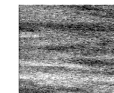
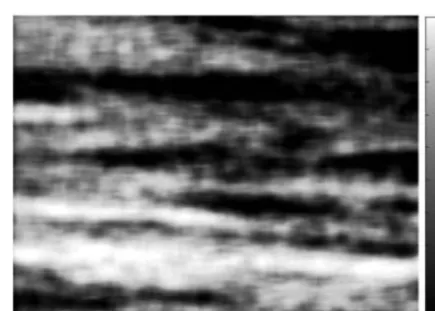
First, the image borders were removed, and the resulting image with the useful area representing thermal image, which covers 550·450 image pixels and includes only the related foil surface area, is shown in Fig. 6. One can notice the speckled (i.e., random noise) nature of the images, and this is due to the relatively low quantum efficiency of the IR radiometer and low infrared signal of the foil: the temperature of the foil was kept at the level of 1–2 K above the temperature of the water, in order to prevent the heating surface effect on the flow. The image is filtered by using the Gaussian low-pass filter and after that enhanced by the standard image processing algorithms (through Image Processing Toolbox, Matlab) for reduc-ing the background illumination effect and histogram equalization. The filtered and enhanced image is shown in the Fig. 7. The main goal of the enhancement is to stretch the histogram of the gray level image, and therefore, to emphasize the difference between the relatively low and high temperature streaks, clearly presented in the en-hanced image. On the right side, the gray levels bar pre-sents the 0–1 scale (i.e., 255 arrow 1) and allows

conversion of the intensity map into a temperature map, shown in Fig. 8 for the subsequent analysis. This image depicts the temperature field of the foil surface with the appropriate color levels, shown in Celsius degrees.

3.3

Analysis of combined measurements

The analysis of the combined PIV and IR technique is performed according to the following procedure:

Fig. 5. Infrared image of the temperature field of the foil surface

Fig. 6. Trimmed image of the temperature field

– PIV images are analyzed by Insight software and the velocity fields are transferred to Matlab;

– IR images are saved as the temperature fields, according to the above image processing and calibration tech-niques;

– Coordinates (i.e., x and z locations), velocity compo-nents (i.e.,uandw), and temperature fieldsTare scaled to the non-dimensional wall units x+,z+,u+,w+,T+: uþ ¼ u=u

wþ ¼ w=u xþ _¼ xu

m

zþ _¼ zu

m

Tþ _¼ DT q00_=qCpu

ð1Þ

whereDT=T)T¥,T¥ is the temperature of the mean flow

in the flume,q00is the Joule heat flux divided by the foil area,u _{is the friction velocity, andmis the kinematic}

viscosity equals to 1·10)6m2/s. The friction velocity was estimated in the previous experiments in the flume (Liberzon et al. 2001; Gurka et al. 2003).

4

Results and discussion

The analysis of the combined measurements begins with the investigation of the fluctuating velocity vector fields versus the fluctuating temperature fields, as in the example in Fig. 9. The fluctuating fields were calculated as the deviation of the instantaneous fields from the ensemble average fields, denoted by theÆÆæoperator. For example, an average streamwise velocity fieldÆu+æis

uþ h i ¼ 1

N

XN

i¼1

uþi ð2Þ

whereNis the number of the experimental realizations. In Fig. 9, the fluctuating velocity and the temperature fields are presented in order to emphasize the turbulent nature of the flow aty+80 (case no. 4 in Table 1). At the same time we mark the streamwise patches of the positive and negative values of the fluctuating temperature (the color levels are the same as in Fig. 8). The relatively large distance between the two measurement planes is due to technical limitations.

Assuming that the thermal patterns on the foil repre-sent the low-speed streaks (Hetsroni et al. 1996; Hetsroni et al. 2001) there is a coupling between the thermal pat-terns and the coherent patpat-terns, detected in the turbulent boundary layer flow (Liberzon et al. 2001; Gurka et al. 2003). The coherent patterns in the velocity fields are described by means of the spanwise variation of the streamwise velocity,u(z). The strong streaky structure in the near-wall region becomes weaker as the outer region of the boundary layer is approached (Smith and Metzler 1983). The spanwise distribution of the streamwise velocity shows the footprint of the bursting process, in-volved with a large-scale vortical motion (Nezu and Nakagawa 1993).

Fig. 10 presents the correlation between the number of thermal elongated patterns (i.e., ‘‘thermal streaks’’) and the number of velocity streaks. The number of these elongated patterns was determined through manual count (Smith and Metzler 1983), by using the automatic tech-nique of Zacksenhouse et al. (2001) and by implementing the recent approach, developed on the basis of the proper orthogonal decomposition (POD) of the flow fields

Fig. 8. Temperature field image

Fig. 9. Fluctuating velocity vector field measured by using PIV

and the fluctuating temperature field measured by using the HFIRI technique

(Liberzon et al. 2001; Gurka et al. 2003). The results of the techniques are in good agreement and the differences were less than 4%. The differences between the results of the techniques at each experimental case are shown in Fig. 10 by vertical error bars. The points represent an average spacing between the streaks in wall units, k+, through the averaging of the results of the different techniques. The abscissa represents various flow condi-tions, according to Table 1. The independence of the spanwise spacing of the thermal patterns on the variety of the flow conditions are in agreement with the fundamental work of Kline et al. (1967) and most of the recent research (e.g., Panton 1997). The average streak spacing based on the thermal patterns was found to be k+160, which is comparable to the popular 100 wall units value. The average spacing, calculated by using the velocity fields, decreases with the increase of flow-rate and the heat flux. It is noteworthy, that the spacing of the velocity deriva-tives does not represent the low-speed streak spacing, since the velocity fields were measured at quite large wall normal distance from the wall. The expansion of the coherent patterns spacing in the velocity fields is caused by two major effects. On one hand, the change in flow rate changes the thickness of the boundary layer. Since our PIV measurements were performed at a fixed physical location (y=10 mm), the normalized distance in wall units,y+is different from one experiment to another, as it is reported in Table 1. For example, the decrease of the flow rate to 270 lpm in case no. 5 defines our field of interest in a lowery+location of about 80 wall units. This is in agreement with the results accumulated by (Fig. 10, Nezu and Nakagawa 1993) from various flows and experimental techniques. The consequential result is shown in Fig. 10, where the average spacing in non-dimensional wall units for the lowest flow rate (case no. 5) is similar to the streak spacing, calculated from the thermal patterns. On the other hand, the change of the heat flux,q00, which was kept as small as possible, influ-ences the flow field close to the wall. The velocity patterns spacing decreases with the increase of the heat flux. One can assume that the foil acts as a heat source, and energy is transferred into the turbulent flow. When the amount

of the energy input into the flow is increased, the increase of the velocity fluctuations affects the velocity streaks spacing.

5

Summary and conclusions

In the present work, we investigated boundary layer flow in a flume by using PIV and IR imaging. Velocity and temperature data, recorded with different frame rates and at different non-dimensional heights, are transferred onto the same spatial non-dimensional grid and compared statistically. The main result is the spanwise spacing be-tween the neighbor patterns of the velocity and the ther-mal streaks. The spacing of the streaks at the proximity of the wall was shown to be independent of the flow condi-tions and the heat flux. However, the spacing of the velocity structures at the fixed physical location (i.e., y=10 mm) and at the different non-dimensional locations (y+) was slightly influenced by the heat flux variations. At the lowest available non-dimensional location ofy+=80 the spanwise spacing calculated from the velocity and tem-perature fields has similar values.

References

Adrian R (1991) Particle-imaging techniques for experimental fluid-mechanics. Annual Rev Fluid Mech 23:261–304

Carlomagno G (1997) Infrared thermography and convective heat transfer. In: Giot M, Mayinger F, Celata G (eds) Experimental heat transfer, fluid mechanics and thermodynamics. Edizioni ETS, Pisa, pp 29–43

De Luca L, Carlomagno G, Buresti G (1990) Boundary layer diag-nostics by means of an infrared scanning radiometer. Exp Fluids 9:121–128

Gurka R, Liberzon A, Hetsroni G (2003) Footprints of funnel vortices in a turbulent boundary layer. In: 56th Annual Meeting of APS. Division of Fluid Dynamics, New Jersey

Hetsroni G, Kowalewski TA, Hu B, Mosyak A (2001) Tracking of coherent thermal structures on a heated wall by means of infrared thermography. Exp Fluids 30:286–294

Hetsroni G, Rozenblit R (1994) Heat transfer to liquid–solid mixture in a flume. Int J Multiphase Flow 20:671–689

Hetsroni G, Rozenblit R, Yarin L (1996) A hot-foil infrared technique for studying the temperature field of a wall. Meas Sci Tech 7:1418– 1427

Fig. 10. Average spacing between the velocity

derivatives patterns and the thermal patterns

associated turbulence in the near-wall region of a turbulent boundary layer. Turbulent Shear Flows 4:223–234

Kim H, Kline S, Reynolds W (1971) The production of turbulence near a smooth wall in a turbulent boundary layer. J Fluid Mech 50:133–160

Kim J (1989) On the structure of pressure fluctuations in simulated turbulent channel flow. J Fluid Mech 205:421–451

Kline S, Reynolds W, Schraub F, Runstadler P (1967) The structure of turbulent boundary layers. J Fluid Mech 30:741–773

Kowalewski TA, Hetsroni G, Mosyak A (2003) Tracking of coherent thermal structures on a heated wall, Part 2: DNS simulation. Exp Fluids 34:390–396. DOI: 10.1007/s00348-002-0574-9

Liberzon A, Gurka R, Hetsroni G (2001) Vorticity characterization in a turbulent boundary layer using PIV and POD analysis. In: Proc 4th Intl Symp PIV. Gottingen, p 1184

Nakagawa H, Nezu I (1981) Structure of space time correlations on bursting phenomena in an open channel flow. J Fluid Mech 104:1–43

vectors correction and derived magnitudes calculation on PIV data. Meas Sci Tech 8:1493–1501

Panton R (1997) Self-sustaining mechanisms of wall turbulence. In: Advances in Fluid Mechanics, vol 15. Computational Mechanics Publications, Southampton, UK

Rashidi M, Banerjee S (1990) Streak characterization and behaviour near wall and interface in open channel flows. J Fluids Eng 112:164–170

Robinson S (1991) Coherent motions in the turbulent boundary layer. Annu Rev Fluid Mech 23:601–639

Smith CR, Metzler SP (1983) The characteristics of low-speed streaks in the near-wall region of a turbulent boundary layer. J Fluid Mech 129:27–54

Zacksenhouse M, Abramovich G, Hetsroni G (2001) Automatic spatial characterization of low-speed streaks from thermal images. Exp Fluids 31(2):229–239