A New Numerical Scheme for Solving Systems of Integro-Differential Equations
Esmail Hesameddini
Department of Mathematics,Shiraz University of Technology, P. O. Box 71555-313, Shiraz, Iran. E-mail: [email protected]
Azam Rahimi
Department of Mathematics, Shiraz University of Technology, P. O. Box 71555-313, Shiraz, Iran. E-mail: [email protected]
Abstract This paper has been devoted to apply the Reconstruction of Variational Iter-ation Method (RVIM) to handle the systems of integro-differential equIter-ations. RVIM has been induced with Laplace transform from the variational itera-tion method (VIM) which was developed from the Inokuti method. Actually, RVIM overcome to shortcoming of VIM method to determine the Lagrange multiplier. So that, RVIM method provides rapidly convergent successive approximations to the exact solution. The advantage of the RVIM in com-parison with other methods is the simplicity of the computation without any restrictive assumptions. Numerical examples are presented to illustrate the procedure. Comparison with the homotopy perturbation method has also been pointed out.
Keywords. System of integro-differential equations, Volterra equation, Reconstruction of varia-tional iteration method, Homotopy perturbation method.
2010 Mathematics Subject Classification. 34K30, 34A12, 45G15.
1. Introduction
Systems of integral equations, linear or nonlinear, appear in scientific appli-cations in engineering, physics, chemistry and populations growth models[4-6, 14, 17]. Studies of systems of integral equations have attracted much concern in applied sciences. Volterra studied the hereditary influences when he was ex-amining a population growth model. The research resulted in a specific topic, where both differential and integral operators appeared together in the same equation. This new type of equation is named as Volterra integro-differential equation, given in the form:
y(i)(x) =f(x) +
Z x
0
k(x, t)u(t)dt,
wherek(x, t) a function of two variables x and t, is called the kernel. In this paper, we will study systems of Volttera integro-differential equations given by:
y(ji)(x) =fj(x, y1(x), y2(x), ..., ym(x)) +
Z x
0
gj(τ, y1(τ), y2(τ), . . . , ym(τ))dτ ,
for j = 1, . . . , m. The functions fj(x, y1(x), y2(x), . . . , ym(x)) are given real
valued functions and unknown functionsy1(x), y2(x), . . . , ym(x) will be deter-mined. A variety of numerical and analytical methods such as series solution method [13], homotopy perturbation method [9, 10], Adomian decomposition method [2, 3, 16] and variational iteration method [1, 12, 15] have been used to solve the systems of integro-differential equations. It is important to point out that these methods have been applied for the separable or difference kernels. In this work, we use the reconstruction of variational iteration method for solving systems of integro-differential equations. This method was first pro-posed by Hesameddini and Latifizadeh [11] and provides rapidly convergent successive approximations of the exact solution if such a closed form solution exists.
2. Preliminaries
For the reader’s convenience, we present some necessary definitions which are used further in this paper.
Definition 2.1. The Laplace transform of f(x) is defined as follows:
F(s) =`{f(t;s)}=
Z ∞
0
e−stf(t)dt.
One of the most important properties of Laplace transform is the convolution of functions f and g. Let the functions f(t) and g(t) be defined for t ≥ 0 , then the convolution of the functionsf and g is denoted by (f ∗g)(t), and is defined as the following integral:
(f∗g)(t) =
Z t
0
f(τ)g(t−τ)dτ .
Let`{f(t)}=F(s),`{g(t)}=G(s), then `{(f ∗g)(t)}=F(s)G(s).Or equiv-alently,`{Rt
0f(τ)g(t−τ)dτ}=F(s)G(s). Conversely,
`−1{F(s)G(s)}=Rt
0f(τ)g(t−τ)dτ.
Definition 2.2. The Laplace transform for the derivatives of f(x) is given by:
`{f(i)(t);s}=siF(s) + m−1
X
k=0
3. Application of the RVIM Method
In this study we consider the following system of integro-differential equa-tions:
y(i)1 (x) =f1(x, y1(x), y2(x), . . . , ym(x)) + Z x
0
g1(τ, y1(τ), Xy2(τ), . . . , ym(τ))dτ ,
y(i)2 (x) =f2(x, y1(x), y2(x), . . . , ym(x)) + Z x
0
g2(τ, y1(τ), y2(τ), . . . , ym(τ))dτ ,
. . .
y(i)m(x) =fm(x, y1(x), y2(x), . . . , ym(x)) + Z x
0
gm(τ, y1(τ), y2(τ), . . . , ym(τ))dτ ,
(3.1)
where gj’s are linear/nonlinear functions of x, y1, y2, . . . , ym and yj(i) is the
derivative ofyj with orderi, subject to the initial conditions:
yj(k)=cjk, 1≤j≤m, 1≤k < i. (3.2) We summarize system (3.1), in the form
yj(i)(x) =Nj(x, y1(x), y2(x), . . . , ym(x)), j = 1, . . . , m, (3.3)
with the zero artificial initial conditions. By taking Laplace transform of the both sides of (3.3), in the usual way and using the artificial initial conditions, the following result is obtained:
si`{yj(x)}=`{Nj(x, y1(x), y2(x), . . . , ym(x))}, j= 1, . . . , m. (3.4) Therefore, we can conclude that:
`{yj(x)}= 1
si`{Nj(x, y1(x), y2(x), . . . , ym(x))}, j= 1, . . . , m. (3.5) Suppose that s1i =H(s), then by using the convolution theorem, one obtains:
`{yj(x)}=H(s)`{Nj(x, y1(x), y2(x), . . . , ym(x))}=`{(h∗Nj)x}, (3.6)
wherej = 1, . . . , m, `−1{H(s)}=h(x). Taking the inverse Laplace transform
to both sides of (3.6), the following result is obtained:
yj(x) =
Z x
0
h(x−τ)Nj(τ, y1(τ), y2(τ), . . . , ym(τ))dτ , j= 1, . . . , m. (3.7)
Now, we must impose the actual initial conditions to obtain the solution of (3.1). Thus we have the following iteration formulation:
yjn+1(x) =yj0(x) +
Z x
0
forj= 1, . . . , m. The valuesy10(x), y20(x), . . . , ym0(x) are given by:
yj0(x) =yj(0) +xy0j(0) +. . .+x ny(n)
j (0)
n! . (3.9)
Therefore, according to the reconstruction of variational iteration method yj(x) is obtained as follows:
yj(x) = limn→∞yjn(x), j= 1, . . . , n, (3.10)
whereyjn(x) indicatesn-th approximation ofyj(x).
4. Numerical Examples
To demonstrate the effectiveness of this method we consider some systems of linear and nonlinear integro-differential equations:
Example 4.1. Consider the following system of Volterra integro-differential equations:
u00(x) =−1−x2−sinx+Rx
0 (u(t) +v(t))dt,
v00(x) = 1−2−sinx−cosx+Rx
0 (u(t)−v(t))dt,
(4.1)
subjected to the initial conditions:
u(0) = 1, u0(0) = 1, v(0) = 0, v0(0) = 2. (4.2)
Applying the Laplace transform to (4.1), the result is as follows:
`{u(x)}= s12`{−1−x2−sinx+
Rx
0 (u(t) +v(t))dt},
`{v(x)}= s12`{1−2−sinx−cosx+
Rx
0 (u(t)−v(t))dt}.
(4.3)
By applying the inverse Laplace transform to both sides of (4.3), result in:
u(x) =Rx
0 (x−t)(−1−t
2−sint+Rt
0(u(τ) +v(τ))dτ)dt,
v(x) =Rx
0 (x−t)(1−2−sint−cost+
Rt
0(u(τ)−v(τ))dτ)dt.
(4.4)
Considering the initial conditions (4.2), the following iterative relations are obtained as:
un+1(x) =u0(x) + Rx
0 (x−t)(−1−t
2−sint+Rt
0(un(τ) +vn(τ))dτ)dt,
vn+1(x) =v0(x) +Rx
0 (x−t)(1−2−sint−cost+ Rt
where u0(x) = 1 +x , v0(x) = 2x and un(x), vn(x) indicates the n-th
ap-proximation of u(x) and v(x) respectively. According to (4.5), after some simplification and substitution, the following sets of relations are resulted:
u1(x) = 1−
x2 2 +
x3 3! +
x4
4! + sinx,
v1(x) =−1 +
x2 2 +
x3 3! −
x4
4! + 2 sinx+ cosx,
u2(x) =x+ (1−
x2 2 +
x4 4! −
x6
6! +. . .),
v2(x) =x+ (x−
x3 3! +
x5 5! −
x7
7! +. . .).
Thus the closed form solutions are as follows:
u(x) = lim
n→∞un(x) =x+ cosx, v(x) = limn→∞vn(x) =x+ sinx.
Now, we will solve this example by the homotopy perturbation method (HPM)[7-10]. To do this, we construct a homotopy function as the following form:
H(u, p) =u(x) + 1 +x2+ sinx−p
Z x
0
(u(t) +v(t))dt,
H(v, p) =v(x)−1 + 2 + sinx+ cosx−p
Z x
0
(u(t)−v(t))dt. (4.6)
The embedding parameterp monotonically increases from 0 to 1. In order to apply this method the following expansion will be used:
u(x) = ∞
X
n=0
pnun(x), v(x) = ∞
X
n=0
pnvn(x), (4.7)
resulted:
u0(x) = 1−
x2
2 − x4
12+ sinx,
v0(x) =−1 +
x2
2 + 2 sinx+ cosx,
u1(x) =−3 +x+
3x2 2 −
x7
2520+ 3 cosx−sinx,
v1(x) = 1−x−
x2 2 + x3 3 − x5 60 − x7
2520+ sinx−cosx,
u2(x) = 2x−
x3 3 + x5 60 + x6 360− x8 20160 − x10
907200−2 sinx,
v2(x) = 2 + 4x−x2−
2x3 3 + x4 12+ x5 30− x6 360+ x8
20160−4 sinx−2 cosx,
u3(x) = 6−2x−3x2+
x3 3 + x4 4 − x5 60 − x6 120+ x7 2520+ x8 6720 − x 13
1556755200−6 cosx+ 2 sinx,
v3(x) =−2 + 2x+x2−
x3 3 − x4 12 + x5 60 + x6 360− x7 2520− x8 20160 + x9 90720 − x 11 9979200 − x13
1556755200+ 2 cosx−2 sinx,
and so on. Therefore, the solutions by the HPM with three terms will be determined as:
u(x) = 4 +x−2x2+x
4 6 − x6 180+ x8 10080− x10 907200 − x13 1556755200 −3 cosx,
v(x) = 5x−2x
3 3 + x5 30 − x7 1260+ x9 90720 − x11 9979200 − x13 1556755200 −3 sinx.
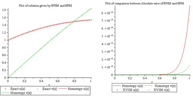
Fig. 1. compares the approximate solutions which are obtained by HPM and RVIM methods. Also the absolute error of these two methods are shown.
Figure 1. Comparison between the solutions of RVIM and HPM
Example 4.2. Now we consider the following system of three Volterra integro-differential equations:
u0(x) = 2 +ex−3e2x+e3x+Rx
0 (6v(t)−3w(t))dt,
v0(x) =ex+ 2e2x−e3x+Rx
0 (3w(t)−u(t))dt,
w0(x) =−ex+e2x+ 3e3x+Rx
0 (u(t)−2v(t))dt,
(4.8)
with the initial conditions:
u(0) = 1, v(0) = 1, w(0) = 1. (4.9)
Applying the Laplace transform to (4.8), the result is as follows:
`{u(x)}= 1s`{2 +ex−3e2x+e3x+Rx
0 (6v(t)−3w(t))dt},
`{v(x)}= 1s`{ex+ 2e2x−e3x+Rx
0 (3w(t)−u(t))dt},
`{w(x)}= 1s`{−ex+e2x+ 3e3x+Rx
0 (u(t)−2v(t))dt}.
(4.10)
Similarly, using the inverse Laplace transform on both sides of (4.10), the following RVIM formula is obtained:
u(x) =R0x(2 +et−3e2t+e3t+R0t(6v(τ)−3w(τ))dτ)dt,
v(x) =R0x(et+ 2e2t−e3t+R0t(3w(τ)−u(τ))dτ)dt,
w(x) =R0x(−et+e2t+ 3e3t+Rt
0 (u(τ)−2v(τ))dτ)dt.
To obtain the approximate solution of (4.8), the iterative relation is considered as
un+1(x) =u0(x) + Rx
0 (2 +e
t−3e2t+e3t+Rt
0(6vn(τ)−3wn(τ))dτ)dt,
vn+1(x) =v0(x) +Rx 0 (e
t+ 2e2t−e3t+Rt
0(3wn(τ)−un(τ))dτ)dt,
wn+1(x) =w0(x) +Rx 0 (−e
t+e2t+ 3e3t+Rt
0(un(τ)−2vn(τ))dτ)dt,
(4.12)
According to (4.9), we consider these initial approximations :
u0(x) = 1, v0(x) = 1, w0(x) = 1.
Then by means of RVIM technique the successive approximate solutions can be obtained:
u1(x) =
7
6 + 2x+ 3 2x
2+ex−3 2e
2x+1 3e
3x,
v1(x) =−
2 3+x
2+ex+e2x−1 3e
3x,
w1(x) =
1 2−
1 2x
2−ex+1 2e
2x−1 3e
3x,
u2(x) = 1 +x+
x2 2! +
x3 3! +
x4
4! +· · · ,
v2(x) = 1 + 2x+
(2x)2 2! +
(2x)3 3! +
(2x)4
4! +· · ·,
w2(x) = 1 + 3x+
(3x)2
2! + (3x)3
3! + (3x)4
4! +....
Therefore, the exact solutions are given by:
u(x) = lim
n→∞un(x) =e x,
v(x) = lim
n→∞vn(x) =e
2x,
w(x) = lim
n→∞wn(x) =e
3x.
can have the following relations:
u0(x) = 1 + 2x+ex−
3 2e
2x+1 3e
3x,
v0(x) = 1 +ex+e2x−
1 3e
3x,
w0(x) = 1−ex+
1 2e
2x+e3x,
u1(x) =−
689 72 −
115 12 x+
3 2x
2+ 9ex+ 9 8e
2x−5 9e
3x,
v1(x) =−
319 108+
29 18x+x
2−1
3x
3−4ex+3 4e
2x+ 8 27e
3x,
w1(x) =
127 72 +
29 12x−
1 2x
2+1
3x
3−ex−7 8e
2x+ 1 9e
3x,
In the same manner, fourth term approximations of the solutions of (4.8) are computed. By considering these approximations, the solutions are approxi-mated as follows:
u(x) =−321126643 1119744 −
53233745 186624 x−
8522971 62208 x
2−1436489
31104 x
3
−212467 20736 x
4−7069
3456x
5− 8023
17280x
6− 509
20160x
7− 3
640x
8
+ 1 1344x
9+ 289ex−711 512e
2x+ 17 2187e
3x,
v(x) =−315159281 1679616 −
53074939 279936 x−
8794217 93312 x
2−1486819
46656 x
3
−274865 31104 x
4−42379
25920x
5− 7397
25920x
6− 1219
30240x
7+ 19
6720x
8
− 19 60480x
9+ 189ex+337 256e
2x− 79 6561e
3x,
w(x) = 836871971 3359232 +
138986593 559872 x+
22766219 186624 x
2+3824473
93312 x
3
+642467 62208x
4+ 101953
51840x
5+20183
51840x
6+ 2293
60480x
7+ 1
13440x
8
− 1
10080x
9−249ex+189 512e
2x+6593 6561e
3x.
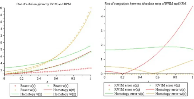
Fig. 2. shows that the RVIM is more efficient than HPM.
Example 4.3.Finally, let us consider the system of nonlinear Volterra integro-differential equation:
u0(x) = 2x+16x4+152 x6+Rx
0 (x−2t)(u
2(t) +v(t))dt,
v0(x) =−2x−16x4+152 x6+R0x(x−2t)(u(t) +v2(t))dt,
Figure 2. Comparison between the RVIM and HPM for
sys-tem (4.8).
subjected to the initial conditions:
u(0) = 1, v(0) = 1. (4.14)
Applying the Laplace transform to (4.13), the result is as follows:
`{u(x)}= 1s`{2x+16x4+152 x6+Rx
0 (x−2t)(u
2(t) +v(t))dt},
`{v(x)}= 1s`{−2x−16x4+ 2 15x6+
Rx
0 (x−2t)(u(t) +v2(t))dt}.
(4.15)
By applying the inverse Laplace transform to both sides of (4.15), result in:
u(x) =R0x(2t+16t4+152 t6+R0t(t−2τ)(u2(τ) +v(τ))dτ)dt,
v(x) =R0x(−2t−16t4+152 t6+R0t(t−2τ)(u(τ) +v2(τ))dτ)dt. (4.16)
Considering the initial conditions (4.14), the following iterative relations are obtained as:
un+1(x) =u0(x) + Rx
0 (2t+ 1 6t
4+ 2 15t
6+Rt
0(t−2τ)(u 2
n(τ) +vn(τ))dτ)dt,
vn+1(x) =v0(x) +Rx 0 (−2t−
1 6t
4+ 2 15t
6+Rt
0(t−2τ)(un(τ) +v 2
n(τ))dτ)dt, (4.17)
According to (4.9), we consider these initial approximations :
Then by means of RVIM technique the successive approximate solutions can be obtained:
u1(x) = 1 +x2+
1 30x
5+ 2
105x
7,
v1(x) = 1−x2−
1 30x
5+ 2
105x
7,
u2(x) = 1 +x2+
1 30x
5+ 2
105x
7,
v2(x) = 1−x2−
1 30x
5+ 2
105x
7.
Therefore, the exact solutions are given by:
u(x) = lim
n→∞un(x) = 1 +x
2+ 1
30x
5+ 2
105x
7,
v(x) = lim
n→∞vn(x) = 1−x
2− 1
30x
5+ 2
105x
7.
As we see in this example, by only two iterations, the method converges to the exact solution and it shows the efficiency of our method for solving nonlinear integro-differential equations.
5. Conclusion
In work, we applied the Reconstruction of Variational Iteration Method (RVIM) for solving the systems of Volterra integro-differential equations. In our method knowing the variational theory is not essential while it was needed in the variational iteration method. It is important to point out that some other methods should be applied for systems with separable or difference ker-nels. Whereas, the RVIM can be used for solving systems of Volterra integro-differential equations with any kind of kernels. By comparing the results of other numerical methods such as homotopy perturbation method, we conclude that the RVIM is more accurate, fast and reliable. Besides , RVIM does not require small parameters; thus, the limitations of the traditional perturbation methods can be eliminated, and the calculations are also simple and straight-forward. These advantages has been confirmed by employing two examples. Therefore, this method is a very effective tool for calculating the exact solu-tions of systems of integro-differential equasolu-tions.
References
[2] J. Biazar, E. Babolian and R. Islam, Solution of the system of Volterra integral equations of the first kind by Adomian decomposition method,Appl. Math. Comput., 139(2003), 249-258.
[3] A. Bratsos, M. Ehrhardt and T. h. Famelis, A discrete Adomian decomposition method for discrete nonlinear Schrodinger equations, Appl. Math. Comput. , 197(2008), 190-205.
[4] Y. S. Choi, R. Lui, An integro-differential equation arising from an electrochemistry model,Quart. Appl. Math. 4(1997) 677686.
[5] J. A. Cuminato, A. D. Fitt, M. J. S. Mphaka, A. Nagamine, A singular integro-differential equation model for dryout in LMFBR boiler tubes, IMA J. Appl. Math. 75(2009) 269290.
[6] C. M. Cushing, Integro-differential Equations and Delay Models in Population Dynam-ics,in: Lecture Notes in Biomathematics, vol. 20, Springer, NewYork, 1977.
[7] D. D. Ganji, A. Rajabi, Assessment of homotopy-perturbation and perturbation meth-ods in heat radiation equations,Int. Commun., Heat and Mass Transfer 33 (3)(2006) 391400.
[8] D. D. Ganji, A. Sadighi, Application of Hes homotopy-perturbation method to nonlinear coupled systems of reaction-diffusion equations, Int. J. Nonlinear Sci. Numer. Simul., 7 (4)(2006) 411418.
[9] A. Golbabai and M. Javidi, Application of He’s homotopy perturbation method for n-th order integro-differential equations,Appl. Math. Comput., 190(2007), 1409-1416. [10] J. H. He, Homotopy perturbation technique, Comput. Math. Appl. Mech. Eng., 178
(1999), 257-262.
[11] E. Hesameddini and H. Latifizadeh, Reconstruction of variational iteration algorithm using the Laplace transform, Int. J. of Non. Sci. and Numer. Sim., 10 (2009), 1365-1370.
[12] A. J. Jerri, Introduction to integral equations with applications,Seconded, Wiley Inter-science, 1999.
[13] K. Maleknejad and Y. Mahmoudi, Taylor polynomial solution of high-order nonlinear Volterra-Fredholm integro-differential equations,Appl. Math. Comput., 145(2003), 641-653.
[14] H. Thieme, A model for the spatial spread of an epidemic, J. Math. Biol., 4 (1977) 337351.
[15] S. Q. Wang and J. H. He, Variational iteration method for solving integro-differential equations,Phys. Lett., 367(2007), 188-191.
[16] A. M. Wazwaz, A reliable modification of Adomaion’s decomposition method, Appl. Math. Comput., 102(1999), 77-86.