Vol. 47 - No. 2 - Fall 2015, pp. 1- 9
٭Corresponding Author, Email: [email protected]
Latency Compensation in Multi Chaotic Systems Using
the Extended OGY Control Method
Ensieh Nobakhti
1and Ali Khaki Sedigh
1*1- Industrial Control Center of Excellence, Department of Systems and Control Engineering, Faculty of Electrical Engineering, K. N. Toosi University of Technology, Tehran, Iran
A
BSTRACTThe problem discussed in this paper is the effect of latency time on the OGY chaos control methodology
in multi chaotic systems. The Smith predictor, rhythmic and memory strategies are embedded in the OGY
chaos control method to encounter loop latency. A comparison study is provided and the advantages of the
Smith predictor approach are clearly evident from the closed loop responses. The complex plants considered
are coupled chaotic maps controlled by the extended OGY scheme. Simulation results are used to show the
effectiveness of the applied Smith predictor scheme structure in multi chaotic systems.
K
EYWORDS1.INTRODUCTION
Delay is a generic problem in the control of chaotic systems. The effective delay time in any feedback loop is the sum of present delay times, e.g. the measurement duration, control design computations, and the system response time to the applied control signal [1, 2, 3].
There are two major chaos control strategies: one is the OGY method (based on linearization of the Poincare´ map [4]) and the other is the Pyragas method (based on a time-delay feedback [5]).
There is another delay- named latency- which is introduced in time-delay feedback methodology. As defined in [6], latency times are the times required to compare the current signal with its time-delayed counterpart and apply the feedback into the system. In an experimental setup, there is always latency involved. Control loop latency is associated with finite propagation speed of the control signal, measurement delays of the system to generate the control signal, or processing times for feedback calculation. In optical or opto-electronic systems, for instance, the length of an optical fiber used to transmit the control signal can become of crucial importance [7]. The same holds for electronic systems such as a fast diode resonator, where a propagation delay acts as a limiting factor [8]. Latency has adverse effects on control systems, which are analysed in [9] and [10]. It is to be noted that delay and latency concepts are interchangeably used in many papers.
It has been shown in [11, 12] that longer latency times reduce the control abilities of the time-delayed feedback control. Similar results were found for the extended time-delayed feedback [13]. Latency times on the OGY controllers is analysed in [1, 2, 3]. It was also shown that the measurement delay problem can be solved systematically for the OGY control and difference control by rhythmic control and memory methods.
One approach to avoid the failure of chaos control due to latency is to simplify the controller as much as possible in order to minimize the control loop latency. An example of this approach includes methods that apply perturbations of a predetermined strength when the system crosses some threshold in the phase space [14, 15]. Using these methods, successful control of fast but low-dimensional chaos was demonstrated. A drawback of these methods is that they rely on the ability of easily defining proper windows and walls in the phase space. This task is conceptually much more difficult in the case of delayed systems where the phase space is infinite dimensional.
These inherent difficulties prevented the applications of such methods to practical delay systems [16].
The primary objective of this paper is to derive by means of a simple example the latency adverse effects on feedback systems and to provide an approach for latency tackling in the face of substantial control-loop latency. The paper is focused on the OGY chaos control methodology and employs the Henon map as a two dimensional chaotic system. Then, Rhythmic control, Memory control, and Smith predictor will be applied in the presence of loop latency and study if these methodologies can overcome the problems caused by the loop latency.
Then, upon the application of such compensating control methods in a single chaotic map, the proposed methods will be applied to complex multi-chaotic interconnected plants. In [17], complex structures containing chaotic subsystems with interactions was considered and an extended OGY method was presented to tackle the interaction effects. In this paper, the Smith predictor structure is appropriately inserted in the proposed structure and the simulation results show the efficiency of the final design methodology.
The paper is organized as follows: A brief review of the OGY control system in its original form and the extended OGY control methodology for interconnected chaotic maps are presented in section 2. In section 3, latency structure is introduced and the stability regions are calculated for the Henon chaotic map, with and without loop latency. In section 4, Rhythmic control method, Memory method, and Smith predictor structure are presented as compensation methods of latency in chaos control systems. In section 5, the presented methods of section 4 are implemented on the Henon chaotic map with latency and simulation results are provided to show the effectiveness of the proposed methodologies. Section 6 contains the implementation results for an interconnected multi- chaotic maps using the extended OGY control. Finally, section 6 concludes the paper.
2.PRILIMINARY THEORIES
OGY is a chaos control technique that does not require the exact dynamical equations governing the system. Moreover, its simple structure is valuable for practical implementations. Let a nonlinear plant be described as
𝒛𝑖+1= 𝑓(𝒛𝑖, 𝑝), (1)
𝐾 = 𝜆𝑢
𝜆𝑢− 1
𝒇𝑢𝑇
𝒇𝑢𝑇𝒈
, (2)
where 𝜆𝑢 is the unstable eigenvalue of the linearized
system, 𝒇𝑢𝑇 is a related vector to the unstable eigenvalue such as
𝒇
𝑢𝑇𝒆
𝑢= 1,
𝒇𝑢𝑇𝒆𝑠= 0.
(3)
𝒆𝑠 and 𝒆𝑢 are the stable and unstable right eigenvectors of the linearized system at system’s fixed point (𝒛𝐹), and 𝒈 is defined as
𝒈 =𝜕𝒛𝐹(𝑝)
𝜕𝑝 |𝑝=𝑝𝑛. (4)
As presented in [17], for control of interconnected chaotic networks, a multivariable control design strategy is needed. The extended OGY, is a methodology to tackle the interconnection effects.
Consider the following chaotic systems that are initially decoupled
{
𝑥𝑛+1= 𝑓1(𝑥𝑛, 𝑦𝑛, 𝑝1)
𝑦𝑛+1= 𝑔1(𝑥𝑛, 𝑦𝑛, 𝑝1)
𝑐1
𝑛= 𝑦𝑛
, (5)
and
{
𝑧𝑛+1= 𝑓2(𝑧𝑛, 𝑤𝑛, 𝑝2)
𝑤𝑛+1= 𝑔2(𝑧𝑛, 𝑤𝑛, 𝑝2)
𝑐2
𝑛= 𝑤𝑛
, (6)
where 𝑥, 𝑦, 𝑧 and 𝑤 are the states, 𝑐1 and 𝑐2 are the outputs, 𝑝1 and 𝑝2 are the control parameters.
Now consider the following interconnected chaotic system:
{
𝑥𝑛+1= 𝑓1(𝑥𝑛, 𝑦𝑛, 𝑝1, 𝛼𝑧𝑛)
𝑦𝑛+1= 𝑔1(𝑥𝑛, 𝑦𝑛, 𝑝1, 𝛼𝑧𝑛)
𝑧𝑛+1= 𝑓2(𝑧𝑛, 𝑤𝑛, 𝑝2, 𝛽𝑥𝑛)
𝑤𝑛+1= 𝑔2(𝑧𝑛, 𝑤𝑛, 𝑝2, 𝛽𝑥𝑛)
, (7)
where 𝛼 and 𝛽 are the scalar interaction factors. The system described by (7) is called a multi-chaotic system. Parameters 𝛼 and 𝛽 affect the controller performance, since they change the actual dynamical equations of each primary system. The extended matrix form for the OGY controller with two manipulated parameters (𝛿𝑝1, 𝛿𝑝2) is
[𝛿𝑝𝛿𝑝1
2] = 2 ((𝜆𝑈− 𝐼)𝐹𝑈
𝑇𝐺)−1𝜆
𝑈𝐹𝑈𝑇𝛿𝜻𝑛, (8)
where 𝜆𝑈 is a matrix whose diagonal terms are the unstable eigenvalues and
[𝐹𝑈 𝐹𝑆]𝑇[𝐸𝑈 𝐸𝑆] = [𝐹𝑈
𝑇
𝐹𝑆𝑇] [𝐸𝑈
𝐸𝑆] = 𝐼, (9)
where 𝐸𝑆 and 𝐸𝑈 are the stable and unstable eigenvectors and 𝐹𝑆 and 𝐹𝑈 are the related basis vectors, respectively.
The extended OGY controller gain for the case of n-manipulated parameters (𝛿𝑝1, … , 𝛿𝑝n) is
[𝛿𝑝⋮1
𝛿𝑝𝑛
] = 𝑛 ((𝜆𝑈− 𝐼)𝐹𝑈𝑇𝐺)
−1
𝜆𝑈𝐹𝑈𝑇𝛿𝜻𝑛. (10)
It was shown in [17] that the proposed procedure can satisfactorily control Multi Chaotic Maps. The matrix
(𝜆𝑈− 𝐼)𝐹𝑈𝑇𝐺 must be non-singular, which is the
controllability condition of the coupled chaotic system.
3.LATENCY STRUCTURE
In a closed loop chaotic system using the OGY control strategy, all latency times of different origins can be
summed up to a new parameter 𝛿. An analytical
expression will be derived for the upper bound of 𝛿, i.e., a maximum latency time, such that the design of an OGY controller is still possible.
To assess the latency effects, the OGY control for the Henon map with one control parameter was considered in [18]. The Henon map can be described by the following equations
{𝑥𝑛+1= 𝑝 − 𝑥𝑛2+ 𝑏𝑦𝑛
𝑦𝑛+1= 𝑥𝑛 , (11)
where 𝑝0= 1.29, 𝑏 = 0.3. The linearized model around the system’s fixed point (𝑥𝐹, 𝑦𝐹) is a 2 × 2 system with
two eigenvalues (𝜆𝑢= −1.8398 , 𝜆𝑠= 0.1630). The
feedback law and updating parameter formula are:
𝛿𝑝𝑛= 𝐾𝛿𝒛𝑛,
𝑝(𝑛) = 𝑝0+ 1.8401(𝑥(𝑛) − 𝑥𝐹)
− 0.3001(𝑦(𝑛) − 𝑦𝐹).
(12)
Therefore, the closed loop feedback law with loop latency, can be written as:
𝑝𝑛= 𝐾𝛿𝒛𝑛−𝛿,
𝑝(𝑛) = 𝑝0+ 1.8401(𝑥(𝑛 − 𝛿) − 𝑥𝐹)
−0.3001(𝑦(𝑛 − 𝛿) − 𝑦𝐹).
(13)
It can be shown that the closed loop system is unstable with 𝛿 = 1. Since the greater amount of latency will cause system instability, it is necessary to use compensation methods in control systems.
fixed point is determined by the eigenvalues of the matrix
𝐴 − 𝐵𝐾. 𝐴 is the Jacobian of the uncontrolled Henon map
and 𝐵 is the sensitivity of the map to some accessible system parameter 𝑝 that is displaced by 𝑝0 from its normal value. The stability of the map depends on the matrix
𝐴 − 𝐵𝐾, which is the Jacobian of the controlled map [18].
To find the region in which the Henon Map presented in (11) may be stabilized with a control vector derived from the OGY method, we have
{ 𝑥𝑛+1= (𝑝0+ 𝑘1𝑥𝑛+ 𝑘2𝑦𝑛) − 𝑥𝑛2+ 𝑏𝑦𝑛
𝑦𝑛+1= 𝑥𝑛 (14)
The linearized closed loop equations of the system around the fixed point is:
[𝑥𝑦𝑛+1
𝑛+1] = [−2𝑥
∗+ 𝑘
1 𝑏 + 𝑘2
1 0 ] [
𝑥𝑛
𝑦𝑛] + [10] 𝑝0. (15)
The characteristic equation of the closed loop system is then equal to
𝜆2+ (2𝑥∗+ 𝑘
1)𝜆 + (𝑘2− 𝑏) = 0. (16)
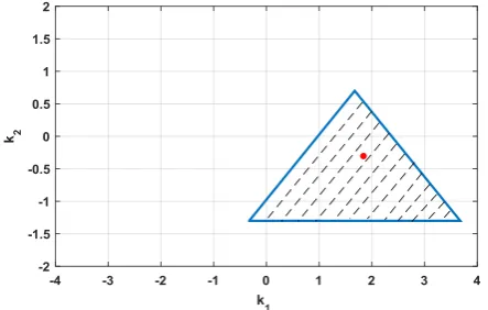
Fig. 1 shows the boundary on the 𝑘1− 𝑘2 plane that can stabilize the chaotic orbit defined in the above equation. If the control parameters are chosen within the region bounded by the triangle and the control algorithm is applied, the system will be stabilized around the fixed point. The small filled circle on the figure shows the calculated state feedback using the OGY control method for the Henon map [17].
Fig. 1.Stability region for the Henon map using state feedback. The borders form the possible selection of 𝒌𝟏 and 𝒌𝟐 to stabilize
the system with state feedback.
Now, let us recalculate the above region for 𝛿 = 1. In this case, the equations of closed loop system are as:
{𝑥𝑛+1= (𝑝0+ 𝑘1𝑥𝑛−1+ 𝑘2𝑦𝑛−1) − 𝑥𝑛2+ 𝑏𝑦𝑛
𝑦𝑛+1= 𝑥𝑛 (17)
The linearized model is:
[
𝑥𝑛+1
𝑦𝑛+1
𝑦𝑛
] = [−2𝑥
∗ 𝑘
1+ 𝑏 𝑘2
1 0 0
0 1 0
] [ 𝑥𝑛
𝑦𝑛
𝑦𝑛−1
] + [10 0] 𝑝0
(18)
The characteristic equation of the closed loop system is then equal to
𝜆3+ 2𝑥∗𝜆2− (𝑘
1+ 𝑏)𝜆 − 𝑘2= 0 (19)
Using the Jury Criterion, the boundary on the 𝑘1− 𝑘2 plane in this case will be as shown in Fig. 2:
Fig. 2.Stability region for the Henon map using state feedback with 𝜹 = 𝟏.
It is clear that the OGY calculated feedback does not lie in the region of possible state feedback elements.
Finally, the 𝑘1− 𝑘2 plane is calculated for 𝛿 = 2 in which the system may be controlled by state feedback. In this case, the linearized closed loop system is presented as:
[
𝑥𝑛+1
𝑦𝑛+1
𝑦𝑛
𝑦𝑛−1
] = [
−2𝑥∗ 𝑏
1 0 𝑘01 𝑘02
0 1
0 0 0 01 0
] [
𝑥𝑛
𝑦𝑛
𝑦𝑛−1
𝑦𝑛−2
] + [ 1 0 0 0
] 𝑝0 (20)
It is easily shown that the closed loop system is unstable for all values of 𝑘1 and 𝑘2.
4.LATENCY COMPENSATION METHODS
A. The Rhythmic OGY Control
As explained in [1, 3], for a 𝛿 time step delay, one can restrict control application rhythmically only every 𝛿 + 1 time-steps, and then leave the system uncontrolled for the remaining time-steps. For the following system with one state (𝑥) and one control parameter (𝑟)
𝑥𝑡+1= 𝑓(𝑥𝑡, 𝑟) (21)
the updating formula for system parameter with feedback gain (𝑘) is computed as
𝑟𝑡= 𝑟0+ 𝑘(𝑥𝑡− 𝑥∗), (22)
where 𝑥∗ is the system fixed point. In the rhythmic control method, 𝑘 is time dependant:
𝑘 = 𝑘(𝑡). (23)
(𝑘 = 𝑘0) and the gain is zero (𝑘 = 0) in remaining iterations. The closed loop characteristic equation in then calculated as
𝑥𝑡+(𝛿+1)= 𝜆𝛿+1𝑥𝑡+ 𝑘0𝜇𝑥𝑡, (24)
where
𝜆 = (𝜕𝑓
𝜕𝑥)𝑥∗,𝑟0 , 𝜇 = (
𝜕𝑓
𝜕𝑟)𝑥∗,𝑟0. (25)
The advantage of this method is that system dimension is not increased and the stability analysis is simpler due to the compact form of (24).
|𝜆𝛿+1+ 𝑘
0𝜇| < 1. (26)
B. Memory OGY Control
In this method, the control parameter (𝑟𝑡) is a linear function of previous states. For the case of 𝛿 = 1 we have:
𝑟𝑡= 𝑘1𝑥𝑡−1+ 𝑘2𝑥𝑡−2+ ⋯ + 𝑘𝑛+1𝑥𝑡−𝑛−1. (27)
For 𝛿 ≥ 2, 𝑘1= ⋯ = 𝑘𝛿−1= 0. If the state vector is
[𝑥𝑡 … 𝑥𝑡−𝑛−1]𝑇, for 𝑛 steps memory and one step delay, the characteristic polynomial is
(𝛼 − 𝜆)𝛼𝑛+1+ ∑ 𝑘
𝑖𝛼𝑛−𝑖= 0 𝑛
𝑖=1
. (28)
This method allows control up to 𝜆𝑚𝑎𝑥= 2 + 𝑛. In [3], the optimal values for 𝑘𝑖 was presented. For more than one step delay, the maximal controllable 𝜆 is reduced and there is no general scheme for optimal selection of 𝑘𝑖. It means that for any arbitrary 𝜆 to be controlled, a memory length of 𝑛 > 𝜆 − 2 is needed.
There is another form for the memory method. If it is possible to use the previously applied control amplitudes 𝑟𝑡−1, 𝑟𝑡−2, . . . , the control parameter will be
𝑟𝑡= 𝑘1𝑥𝑡−1+ 𝑘2𝑥𝑡−2+ ⋯ + 𝑘𝛿𝑥𝑡−𝛿+ 𝜂1𝑟𝑡−1
+ ⋯ + 𝜂𝛿𝑟𝑡−𝛿, (29)
in which 𝑘1= ⋯ = 𝑘𝛿−1= 0 for 𝛿 ≥ 2 [3].
C.Smith Predictor Structure
The presence of a large input delay 𝑘 implies that the control action will be equally delayed [19]. Suppose that 𝐺(𝑧−1) is the system transfer function with delay 𝑧−𝑘. A practical and yet well established approach to delay control is the Smith predictor method.
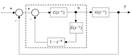
Fig. 3 represents a schematic structure for the Smith predictor. 𝐺̃(𝑧−1) is delay free plant transfer function and 𝐶(𝑧−1) is a designed controller that is considered satisfactory.
Fig. 3.Block diagram of the Smith predictor algorithm.
Using this structure, the controller generates the correct control action.
5.CONTROLLING LATENCY IN HENON MAP
In this section, the compensation control methods described in section 4 are applied to the Henon map.
A. Rhythmic Control for Henon Map
Rhythmic control equation for the Henon map can be written as:
𝛿𝑝𝑛= 𝐾𝑛𝛿𝒛𝑛−𝛿 , 𝛿 ≥ 1, (30)
{𝐾𝑛= 𝐾 , 𝑛 = 𝑖 × (𝛿 + 1), 𝑖 = 0,1,2, …
𝐾𝑛= 0 , 𝑂. 𝑊. ,
(31)
{𝑥𝑛+𝛿+1= 𝑝0+ 𝐾1(𝑥𝑛− 𝑥∗) + 𝐾2(𝑦𝑛− 𝑦∗) − 𝑥𝑛2+ 𝑏𝑦𝑛 𝑦𝑛+1= 𝑥𝑛
(32)
Let 𝑍𝑛=[𝑥𝑛 𝑦𝑛]𝑇 be the state vector, then 𝑍𝑛+1=
𝑍𝑛= 𝑍∗ at the system fixed point. Using (32), the following equation will be obtained:
𝑍𝑛+(𝛿+1)=𝑍∗+(𝐴𝛿+1+ 𝐵𝐾)(𝑍𝑛− 𝑍∗), (33)
where
𝐴 = (𝜕𝑓
𝜕𝑍)𝑍∗,𝑝0= [−2
𝑥∗ 𝑏
1 0] ,
𝐵 = (𝜕𝑓
𝜕𝑝)𝑍∗,𝑝0 = [10].
(34)
For the Henon map with 𝛿 = 1, we have
𝐴2+ 𝐵𝐾 = [4𝑥∗2+ 𝑏 + 𝑘1 −2𝑥∗𝑏 +𝑘2
−2𝑥∗ 𝑏 ], (35)
The closed loop eigenvalues are
𝜆1= 5.2252 , 𝜆2= 0.0266, (36)
which means that the closed loop with loop latency is not stable. In addition, simulation results show that this compensation method is not suitable for a Henon map with 𝛿 = 1.
B. Memory Method for Henon Map
(like the OGY strategy), hence an additional feedback term is used:
𝑝𝑛= 𝑘1𝑥𝑛−1+ 𝑘2𝑦𝑛−1+ 𝑘3𝑝𝑛−1. (37)
The closed loop linearized system with
[𝑥𝑛 𝑦𝑛 𝑦𝑛−1 𝑝𝑛−1]𝑇 as the state vector, gives
𝜆4+ (2𝑥∗− 𝑘
3)𝜆3+ (−𝑘1− 2𝑥∗𝑘3− 𝑏)𝜆2
+ (𝑏𝑘3− 𝑘2)𝜆 = 0. (38)
In this case, there is a solution to have the closed loop eigenvalues as 𝜆1= 𝜆2= 0 and 𝜆3= 𝜆𝑠, by the following design:
𝑘1= −3.38498 , 𝑘2= 0.55194, 𝑘3= 1.8398 .
Simulation results of the states and control parameter are shown in Fig. 4.
For 𝛿 = 2, there is no solution with the following
control law:
𝑝𝑛= 𝑘1𝑥𝑛−2+ 𝑘2𝑦𝑛−2+ 𝑘3𝑝𝑛−1. (39)
But using additional terms of the previously applied control parameters as:
𝑝𝑛= 𝑘1𝑥𝑛−2+ 𝑘2𝑦𝑛−2+ 𝑘3𝑝𝑛−1+ 𝑘4𝑝𝑛−2, (40)
there is a controller with satisfactory performance. In this case, the characteristic polynomial of the closed loop system is
𝜆6+ (2𝑥∗− 𝑘
3)𝜆5+ (−𝑘4− 2𝑘3𝑥∗− 𝑏)𝜆4
+ (𝑏𝑘3− 𝑘1− 2𝑘4𝑥∗)𝜆3
+ (𝑏𝑘4− 𝑘2) = 0.
(41)
Using a controller with the following parameters
𝑘1= 6.2279 , 𝑘2= −1.0155 ,
𝑘3= 1.8398 , 𝑘4= −3.3850,
(42)
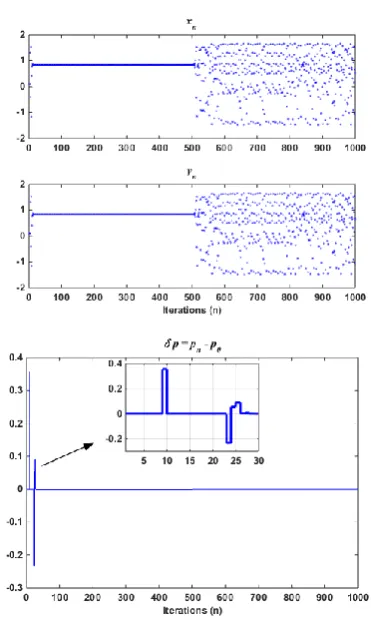
the stable eigenvalues of the open loop system remain unchanged and the unstable ones will be zero in the closed loop system. Simulation results of the states and control parameter are shown in Fig. 5.
Fig. 4.Simulation of the Henon map with delay 𝜹 = 𝟏 by the memory method.
C.Smith Predictor for Henon Map
Fig. 6 presents the block diagram form of the Henon Map with loop latency.
Fig. 6.Block diagram form of the Henon map with delay.
Closed loop instability is inevitable even with 𝛿 = 1. The Smith predictor proposed to compensate the Henon system with latency is applied and simulation results indicate the success of this methodology. Fig. 7 demonstrates the system states and control parameter deviations for 𝛿 = 2.
The results show that the Smith predictor compensates for the system’s latency efficiently.
6.COMPENSATION IN MULTI CHATIC MAPS
For coupled Henon and Ushiki maps, the system equations will be as:
{
𝑥𝑛+1= 𝑝 − 𝑥𝑛2+ 0.3𝑦𝑛
𝑦𝑛+1= 𝑥𝑛+ 𝛼𝑧𝑛
𝑧𝑛+1= (𝑎 − 𝑧𝑛− 0.06𝑤𝑛)𝑧𝑛
𝑤𝑛+1= (2.5 − 0.4𝑧𝑛− 𝑤n)𝑤𝑛+ 𝛽𝑥𝑛
, (43)
where 𝑥, 𝑦, 𝑧 and 𝑤 are the states, 𝑝 and 𝑎 are the control parameters, and 𝛼 and 𝛽 are the state interaction parameters between the two chaotic map dynamics [17].
As was shown in [17], the basic OGY method is not suitable for complex chaotic maps with interconnections and so the extended OGY methodology must be used. Simulation results show that the latency time can easily destabilize the controlled coupled Henon and Ushiki maps using the extended OGY methodology.
For 𝛿 = 1, the states diverge and therefore a
compensation method is needed. Hence, the proposed methods of section 4 will be applied to the system described in (43).
A.Rhythmic Control in Coupled Multi Chaotic Maps
For the linearized system described in (43) around the fixed point, with 𝛼 = 𝛽 = 0.05,
Fig. 7.Smith predictor applied to the Henon map with latency 𝜹 =2.
𝐴 = [
−1.7142 0.3
1 0 0.05 00 0
0 0
0.0500 0 −1.9752 −0.1785−0.1654 0.4827
],
𝐵 = [ 1 0 0 0 0 2.9752
0 0
] ,
𝐾
= [ 1.2915−0.0161 −0.0124−0.6919 0.1240 −0.01890.8979 0.0606 ].
(44)
The control feedback law in this case is:
[𝛿𝑝𝑛
𝛿𝑎𝑛] = 𝐾𝑛[
𝛿𝒙𝑛−𝛿
𝛿𝒚𝑛−𝛿
𝛿𝒛𝑛−𝛿
𝛿𝒘𝑛−𝛿
] , 𝛿 ≥ 1, (45)
{𝐾𝑛= 𝐾 , 𝑛 = 𝑖 × (𝛿 + 1), 𝑖 = 0,1,2, …
𝐾𝑛= 0 , 𝑂. 𝑊. . (46)
The eigenvalues of 𝐴2+ 𝐵𝐾 are 4.9772, 6.6158,
−0.1428, and 0.2448 and the closed loop system is
B. Memory Method in Coupled Multi Chaotic Maps
In this case, the control feedback law is
[𝛿𝑝𝑛
𝛿𝑎𝑛] = 𝐾𝑛[
𝛿𝒙𝑛−𝛿
𝛿𝒚𝑛−𝛿
𝛿𝒛𝑛−𝛿
𝛿𝒘𝑛−𝛿
] , 𝛿 ≥ 1, (47)
[𝑝𝑎𝑛
𝑛] = [
𝑘1 𝑘2
𝑘5 𝑘6
𝑘3 𝑘4
𝑘7 𝑘8] [
𝑥𝑛−1
𝑦𝑛−1
𝑧𝑛−1
𝑤𝑛−1
]
+ [𝑞𝑞1 𝑞2
3 𝑞4] [
𝑝𝑛−1
𝑎𝑛−1].
(48)
If the state vector of the original system is defined as
𝑍𝑛= [𝑥𝑛 𝑦𝑛 𝑧𝑛 𝑤𝑛]𝑇 and the input control
parameter vector is 𝑃𝑛= [𝑝𝑛 𝑎𝑛]𝑇, then the state space vector for applying memory method for system described in (43) with latency time 𝛿 = 1 via memory method will be:
[𝑍𝑍𝑛−1𝑛
𝑃𝑛−1
]
This choice will form a system matrix with 10 × 10 dimension which leads to difficulties in calculating a suitable state feedback to set all closed loop eigenvalues to zero (except the stable open loop ones which remain unchanged). As it is illustrated in this example, calculation burden is a limiting feature of this methodology.
C.Smith Predictor in Coupled Multi Chaotic Maps
In this section, Smith predictor is used for complex multi-chaotic systems. In order to examine the effect of this compensator, Smith predictor is applied to the system described in (43) as presented in Fig. 8.
Fig. 8.Block diagram for Smith predictor applied in multi chaotic system.
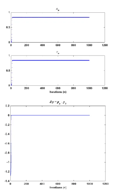
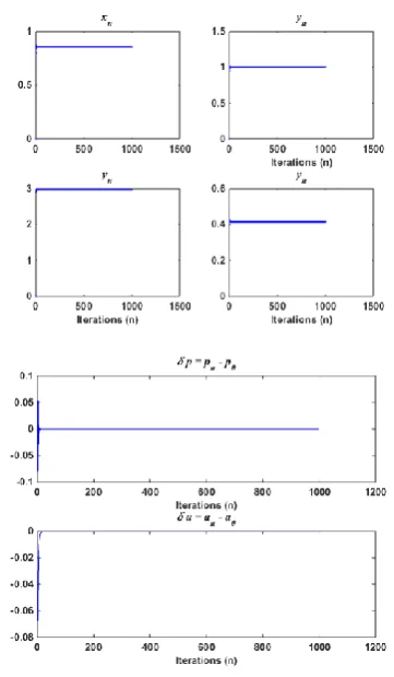
Fig. 9.States and two control parameters of interconnected maps described in (43) using extended OGY method as the controller and Smith predictor as latency time compensator.
𝑥, 𝑦, 𝑧 and 𝑤 are the states, 𝑝 and 𝑎 are the control parameters, 𝑛 is the current iteration, and 𝛿 is the latency of the multi chaotic system.
Simulation results in Fig. 9 indicate that Smith predictor can be an appropriate compensator for latency in multi chaotic systems.
7.CONCLUSIONS
In this paper, the problem of controlling chaotic systems in presence of loop latency was considered. The latency compensation methods were reviewed and they have been applied to both simple Henon map using OGY chaos control and a complex chaotic structure. For complex chaotic maps, the extended OGY control methodology must be used. The compensation methods analysed in this paper are Rhythmic control, Memory Method and Smith predictor. In Rhythmic control, the
control signal was injected in every (𝛿 + 1)-fold
there were some problems in application such as instability and increasing the closed loop systems dimensions. It should be noted that in the Memory method, there is no rule for selecting the number of previous states/parameters to be involved in the control signal. Also, it is not a suitable solution for high dimensional systems. As it is shown in multi chaotic example, the dimension of added items (parameters or states) in the state vector of the system causes difficulties in calculations for finding an OGY controller. The Smith predictor is a structure in which the designed controller is not changed and the loop latency can be compensated. In both simple and complex chaotic maps, Smith predictor has a closed loop satisfactory performance in conjunction with the OGY controllers.
REFERENCES
[1] J.C. Claussen, and H.G. Schuster, “Improved
Control of Delayed Measured Systems,” Physical Review E, 70: 056225, 2004.
[2] J.C. Claussen, “Delayed Measurements in
Pincare-Based Chaos Control,” Physical Review E, 70:046128, 2005.
[3] E. Scholl, and H.G. Schuster, Hand Book of
Chaos, Wiley, 2008.
[4] E. Ott, C. Grebogi, and J.A. Yorke, “Controlling chaos,” Physical Review Letters, vol. 64, pp. 1196–1199, 1990.
[5] K. Pyragas, “Continuous control of chaos by self- controlling feedback,” Physics Letters A, vol. 170, pp. 421-428, 1992.
[6] P. Hovel, “Effects of chaos control and latency in time-delay feedback methods,” PhD Thesis, 2004.
[7] S. Schikora, P. Hövel, H.J. Wünsche, E. Schöll, and F. Henneberger, “All-optical noninvasive control of unstable steady states in a semiconductor laser,” Physical Review Letters, 97:213902, 2006.
[8] D.J. Gauthier, D.W. Sukow, H.M. Concannon, and
J.E.S. Socolar, “Stabilizing unstable periodic orbits in a fast diode resonator using continuous time-delay autosynchronization,” Physical Review E, 50:2343, 1994.
[9] D.W. Sukow, M.E. Bleich, D.J. Gauthier, and
J.E.S. Socolar, “Controlling chaos in a fast diode resonator using time-delay autosynchronization:
experimental observations and theoretical
analysis,” Chaos, 7:560, 1997.
[10] J.N. Blakely, “Experimental Control of a Fast Chaotic Time-Delay Opto-Electronic Device,” PhD Thesis, Duke University, 2003.
[11] W. Just, E. Reibold, H. Benner, K. Kacperski, P. Fronczak, and J. Holyst, “Limits of time delayed feedback control,” Physics Letters A, 254:158, 1999.
[12] W. Just, D. Reckwerth, E. Reibold, and H. Benner,
“Influence of control loop latency on time delayed feedback control,” Physics Letters E, 59:2826, 1999.
[13] P. Hövel, and J.E.S. Socolar, “Stability domains for time-delay feedback control with latency,” Physics Letters E 68:036206, 2003.
[14] N. Corron, B. Hopper, and S. Pethel, “Limiter control of a chaotic RF transistor oscillator,” International Journal of Bifurcation and Chaos, vol. 13, no. 04, pp. 957-961, 2003.
[15] K. Myneni, T.A. Barr, N.J. Corron, and S.D.
Pethel, “New method for the control of fast chaotic oscillations,” Physical Review Letters, 83: 2175, 1999.
[16] L. Illing, D.J. Gauthier, and J.N. Blakely,
“Controlling fast chaos in optoelectronic delay dynamical systems,” Hand Book of Chaos Control, Second Edition, Wiley, 2008.
[17] E. Nobakhti, A. Khaki-Sedigh, and N. Vasegh, “Control of Multi-Chaotic Systems using the Extended OGY Method,” International Journal of Bifurcation and Chaos, 25: 1550096, 2015.
[18] L. Jentoft, and Y. Li, “Stabilizing the Henon Map
with the OGY Algorithm,” Report, Olin College of Engineering, 2008.