APPLICATION OF A COST-DRIVEN OPTIMIZATION
METHOD IN BEER BREWING PROCESS
Mohammad Bameni Moghadam
Department of Statistics, Allameh Tabatabaee University Tehran, Iran, [email protected]
(Received: December 11, 2002 – Accepted in Revised Form: December 25, 2003)
Abstract The final quality and cost of a manufactured product are determined to a large extent by the engineering design of the product and its production process through activities of off-line quality control methods, namely, System Design, Parameter Design and Tolerance Design. However, in the context of most non-industrialized countries, the off-line quality activities of product design and system design of production process design stages are negligible if not absent. Thus, whatever quality control activities there are in these countries should be confined only to conducting parameter (robust) design of manufacturing process design and on-line quality control activities. Out of these two activities, Robust Design is the most economical method as it increases quality and/or reduces costs without imposing any further investment in factors of production. It is in this context that robust design as an optimization method has been used to improve the product quality of cleaning sub-process of beer brewing sub-process of Behnoosh Company in which 358% improvement over the current condition has been achieved.
Key Words Robust Design, System Design, Parameter Design, Tolerance Design, Optimization
ﻩﺪﻴﻜﭼ
ﻩﺪﻴﻜﭼ
ﻩﺪﻴﻜﭼ
ﻩﺪﻴﻜﭼ
ﺖﺧﺎﺳﺪﻨﻳﺍﺮﻓﻭﻝﻮﺼﺤﻣﻲﺣﺍﺮﻃﻂﺳﻮﺗﻱﺩﺎﻳﺯﺭﺎﻴﺴﺑﺪﺣﺎﺗﻝﻮﺼﺤﻣﻚﻳﻲﻳﺎﻬﻧﻱﺎﻫﻪﻨﻳﺰﻫﻭﺖﻴﻔﻴﻛ ﻱﺮﺘﻣﺍﺭﺎﭘﻲﺣﺍﺮﻃ،ﻪﻧﺎﻣﺎﺳﻲﺣﺍﺮﻃﻪﻧﺎﮔﻪﺳﻞﺣﺍﺮﻣﻲﻃﺖﺧﺎﺳﺯﺍﻞﺒﻗﻱﺯﺎﺳﻪﻨﻴﻬﺑﺎﻳﺖﻴﻔﻴﻛﻝﺮﺘﻨﻛﺵﻭﺭﻖﻳﺮﻃﺯﺍ
ﻲﻣﺕﺭﻮﺻﻱﺭﺍﺩﺍﻭﺭﻲﺣﺍﺮﻃﻭ ﺩﺮﻳﺬﭘ
.
ﺖﻴﻟﺎﻌﻓ،ﻲﺘﻌﻨﺻﺮﻴﻏﻱﺎﻫﺭﻮﺸﻛﺐﻠﻏﺍﺭﺩﺎﻣﺍ
،ﻝﻮﺼﺤﻣﻲﺣﺍﺮﻃﻲﻌﻗﺍﻭﻱﺎﻫ
ﺖﺳﺍ ﺮﻈﻨﻓﺮﺻﻞﺑﺎﻗﺎﻳﻭﺩﺭﺍﺪﻧ ﺩﻮﺟﻭﺎﻳﺖﺧﺎﺳﺪﻨﻳﺍﺮﻓﻲﺣﺍﺮﻃﻱﺭﺍﺩﺍﻭﺭﻭﻪﻧﺎﻣﺎﺳﻲﺣﺍﺮﻃ
. ﻱﺎﻫﺖﻴﻟﺎﻌﻓ،ﻦﻳﺍﺮﺑﺎﻨﺑ
ﻱﺎﻫﺵﻭﺭﻭﺖﺧﺎﺳﺪﻨﻳﺍﺮﻓﻲﺣﺍﺮﻃﺭﺩﻱﺮﺘﻣﺍﺭﺎﭘﻲﺣﺍﺮﻃﻪﺑﺩﻭﺪﺤﻣﺎﻫﺭﻮﺸﻛﻦﻳﺍﺭﺩﻱﺯﺎﺳﻪﻨﻴﻬﺑﺎﻳﺖﻴﻔﻴﻛﻝﺮﺘﻨﻛ
ﻲﻣﺖﺧﺎﺳ ﻦﻴﺣﺖﻴﻔﻴﻛ ﻝﺮﺘﻨﻛ ﺩﻮﺷ
.
ﻭﺩ ﻦﻳﺍ ﺯﺍ
ﺭﺍﻮﺘﺳﺍﺡﺮﻃﺵﻭﺭ ،ﺖﻴﻟﺎﻌﻓﻉﻮﻧ
)
ﻱﺮﺘﻣﺍﺭﺎﭘﻲﺣﺍﺮﻃ
( ﻱﺩﺎﺼﺘﻗﺍ ،
ﺖﺳﺍﺖﻴﻔﻴﻛﻝﺮﺘﻨﻛﻥﻮﻨﻓﺯﺍﺩﻮﺟﻮﻣﺭﺎﻜﻫﺍﺭﻦﻳﺮﺗ
. ﺭﺩﻲﻓﺎﺿﺍﻱﺭﺍﺬﮔﻪﻳﺎﻣﺮﺳﻪﻨﻳﺰﻫﻞﻴﻤﺤﺗﻥﻭﺪﺑﺵﻭﺭﻦﻳﺍﺍﺮﻳﺯ
ﻲﻣ ﺚﻋﺎﺑ ﺍﺭﺖﻤﻴﻗ ﺶﻫﺎﻛﺎﻳ ﻭ ﺖﻴﻔﻴﻛ ﺶﻳﺍﺰﻓﺍ ،ﺪﻴﻟﻮﺗ ﻞﻣﺍﻮﻋﺎﺑ ﻁﺎﺒﺗﺭﺍ ﺩﻮﺷ
. ﻲﻳﻮﺟ ﻩﺮﻬﺑ ﻖﻳﺮﻃ ﺯﺍ ﺵﻭﺭﻦﻳﺍ
ﻲﻄﺧﺮﻴﻏﻱﺎﻫﺮﺛﺍ
ﻲﺣﺍﺮﻃﻱﺎﻫﺮﺘﻣﺍﺭﺎﭘﻦﻴﺑﺩﻮﺟﻮﻣ
)
ﻝﺮﺘﻨﻛﻞﺑﺎﻗﻞﻣﺍﻮﻋ
(
ﻲﺘﺣﺎﻳﺖﺧﺎﺳﻂﻴﺤﻣﺭﺩﺵﺎﺸﺘﻏﺍﻞﻣﺍﻮﻋ،
ﺐﺒﺳ ﺍﺭ ﻱﺯﺎﺳ ﻪﻨﻴﻬﻳ ،ﺪﻨﻳﺍﺮﻓ ﺎﻳ ﻝﻮﺼﺤﻣ ﺖﻴﻔﻴﻛ ﺢﻄﺳ ﻩﺪﻨﻨﻛ ﻦﻴﻴﻌﺗ ﻲﻔﻴﻛ ﻱﺎﻫ ﻪﺼﺨﺸﻣ ﻭ ﻱﺮﻴﮔﺭﺎﻜﺑ ﻂﻴﺤﻣ ﻲﻣ ﺩﺩﺮﮔ
. ﻑﺬﺣﻖﻳﺮﻃ ﺯﺍﺍﺭﻱﺯﺎﺳ ﻪﻨﻴﻬﺑ ﻪﻛﻲﺣﺍﺮﻃﺭﺩ ﺩﻮﺟﻮﻣﺮﮕﻳﺩ ﻱﺎﻫ ﺵﻭﺭﺲﻜﻋﺮﺑ ،ﺮﮕﻳﺩﺕﺭﺎﺒﻋ ﻪﺑ ﺎﻳ
ﻲﻣ ﻡﺎﺠﻧﺍ ﺖﻠﻋ ﻝﺮﺘﻨﻛ
ﻪﺑ ﺖﺒﺴﻧ ﺎﻫ ﻪﻧﺎﻣﺎﺳ ﻥﺩﻮﻤﻧﺱﺎﺴﺣ ﺮﻴﻏ ﻖﻳﺮﻃ ﺯﺍﺍﺭ ﻑﺪﻫ ﻪﺑ ﻲﺑﺎﻴﺘﺳﺩ ﺵﻭﺭﻦﻳﺍ ،ﺪﻨﻫﺩ
ﻲﻣ ﻖﻘﺤﺗ ﺕﺎﺷﺎﺸﺘﻏﺍ ﺪﺸﺨﺑ
. ﻱﺭﺎﺟﻮﺑ ﺪﻨﻳﺍﺮﻓ ﺮﻳﺯ ﻱﺯﺎﺳ ﻪﻨﻴﻬﺑ ﻱﺍﺮﺑ ﺭﺍﻮﺘﺳﺍ ﺡﺮﻃﺵﻭﺭ ﺩﺮﺑﺭﺎﻛ ﻖﻴﻘﺤﺗ ﻦﻳﺍ ﺭﺩ
ﻴﻔﻴﻛﺶﻳﺍﺰﻓﺍﺭﺩﺵﻭﺭﻱﺪﻨﻤﻧﺍﻮﺗﺎﺗﻩﺪﺷﻩﺩﻮﻣﺯﺁﺵﻮﻨﻬﺑﺖﻛﺮﺷﻱﺯﺎﺳﻮﺠﺑﺁﺕﺎﻴﻠﻤﻋ
ﻪﻨﻳﺰﻫﺶﻫﺎﻛﻭﻝﻮﺼﺤﻣﺖ
ﺩﻮﺷ ﺭﺎﻜﺷﺁﻲﻳﺍﺬﻏﻊﻳﺎﻨﺻﻱﺪﻴﻟﻮﺗﺕﻻﻮﺼﺤﻣ ﻞﻛ
. ﺮﮕﻧﺎﻴﺑﻩﺪﻣﺁﺖﺳﺪﺑﺞﻳﺎﺘﻧ ٣٥٨
ﻊﺿﻭ ﻪﺑﺖﺒﺴﻧ ﺩﻮﺒﻬﺑﺪﺻﺭﺩ
ﺖﺳﺍﺩﻮﺟﻮﻣ
.
1. INTRODUCTION
The traditional role of quality control is basically to eliminate from production lines those parts that do not conform to specifications, and to inspect and test finished products for defects. Given this definition, quality control is almost limited to inspecting and testing on a detailing or sampling basis. However, the increased emphasis on “high quality” products at lower cost, combined with the
According to one of these redefined quality control activities which is called Parameter (Robust) Design, the final quality and cost of a manufactured product are determined to a large extent by the engineering design of the product and its production process through activities of off-line quality control methods. However, in the context of most non-industrialized countries, the off-line quality control activities of product design and system design of production process design stages are negligible if not absent. So, whatever quality control activities there are in these countries are confined only to conducting parameter design of manufacturing process design and on-line quality control activities.
It is in this context that an attempt was
made to improve the output of one of the
sub-processes of beer production, namely, cleaning
and grading process by using the method of
Parameter Design. In this regard, it is worth
mentioning that the wonderful obtained result
was achieved under unimaginable vast
conditions of the process without imposing
any further cost in factors of production.
2. METHODOLOGY
Designing high-quality products and processes at low cost is an economic and technological challenge to an engineer. A systematic and efficient way to meet this challenge is a new method of design optimization for performance, quality, and cost. The optimization method, called Robust Design, consists of
1. making product performance insensitive to raw material variation, thus allowing the use of low grade material and components in most cases, 2. m a k i n g d e s i g n s r o b u s t a g a i n s t
manufacturing variation, thus reducing labor and material cost for rework and scrap,
3. making the design least sensitive to the variation in operating environment, thus improving reliability and reducing operating cost and
4. using a new structured development process so that engineering time is used most productively.
The founder of the Robust Design methodology is Professor Genichi Taguchi. His approach includes both a philosophy and a methodology. The essence of philosophy is that any inquiry into improving the quality of products and processes should begin with an analysis of their respective designs. The methodology proposed to establish the optimal design parameters for the major design characteristics of products and processes is divided into three distinct steps or activities: system design, parameter design, and tolerance design.
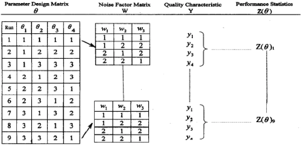
some reasons like manufacturing and / or operational costs, the system should be insensitive to them also. The noise factor matrix specifies the test levels of such noise factors. Its columns represent the noise factors and its rows represent different combinations of noise levels. Therefore, the complete experiment consists of a combination of the design parameter and the noise factor matrices (See Figure 1). Each test run of the design parameter matrix is crossed with all rows of the noise factor matrix. So that in the example in figure 1, there are four trials in each test run – one for each combination of noise levels in the noise factor matrix. The performance characteristic is evaluated for each of the four trials in each of the nine test runs. Thus, the variation in multiple values of the performance characteristic minimize the product (or process) performance variation at the given design parameter settings [1,2,3,4,5]. In the case of continuous performance characteristics (as shown in Figure 1), multiple observations from each test run of the design parameter matrix are used to compute a criterion called Performance Statistic. A performance statistic estimates the effect of noise factors. The computed values of a performance statistic are
used to predict better settings of the design parameters. The prediction is subsequently verified by a confirmation experiment. The initial design parameter settings are not changed unless the veracity of the prediction has been verified. Several iterations of such parameter design experiments may be required to identify the design parameters settings at which the effect of noise factors is sufficiently small.
Parameter design experiments can be done in one of two ways: through physical experiments or through computer simulation trials. These experiments can be done with a computer when the function Y= f (
θ
,
ω
)-relating performance characteristic Y to design parametersθ
, and noise factorsω
-can be numerically evaluated [5, 6, 7]. Taguchi recommends the use of “orthogonal arrays” for constructing the design parameter and the noise factor matrices. All common factorial and fractional factorial plans of experiments are orthogonal arrays, but not all orthogonal arrays are common fractional factorial plans. Kackar, with discussions and response, and Hunter have discussed the use of orthogonal arrays from the statistical viewpoint.3. BEER PRODUCTION PROCESS IN BEHNOOSH COMPANY
The present Behnoosh Company was established in 1967 in the name of SKOL. Essentially, it was an alcoholic beer producer. However, after Islamic Revolution in 1979, the production has been converted into non-alcoholic beer and different types of beverages. The process of beer production, which is commonly referred to as “Beer Brewing” and may use different types of cereals, consists of following sub-processes: 1. Cleaning and Grading,
2. Malting,
3. Mashing,
4. Boiling,
5. Fermenting, and 5. Filtering and Bottling.
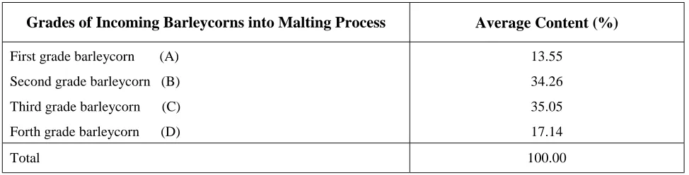
In the first sub-process of non-alcoholic beer production in Behnoosh, which uses barleycorn, unwanted materials like dust, stones, straws, etc., are removed and grading is taken place to have specified barleycorns. In Malting process, the cleaned and graded barleycorns are soaked in water and treated in a way to germinate and then dried-germinated barleycorns, which are called malt, will be produced. In Mashing process the malt is crushed and treated with hot water (wort) to convert the malt-starch into sugar. Then, in boiling process, the wort is boiled vigorously with hopes to give the bitterness and desired TABLE 1. Average of Different Grades of Outgoing Barleycorns to Malting Process under Current Condition.
Grades of Incoming Barleycorns into Malting Process Average Content (%)
First grade barleycorn (A)
Second grade barleycorn (B)
Third grade barleycorn (C)
Forth grade barleycorn (D)
13.55
34.26
35.05
17.14
Total 100.00
TABLE 2. Controllable Factors and Their Levels.
Factors and Levels
Process
Controllable factor or
Design Parameter Levels
I II III
Separator I
1. Air Suction 2. Speed 3. Feeding Rate
3 cm
τ
-3 cmτ
′-0.5 cm3.5 cm
τ
cmτ
′ cmτ
+ 3 cmτ
′ + 0.5 cmSeparator II 4. Vibration 5. Air Suction
6o
40o
7o
50o
8o
60o
Grader
6. Upper Control Gradiometer 7. Lower Control Gradiometer 8. Speed
0o
5o
τ
′′ - 3 cm2o
8o
τ
′′ cm4o
color to beer. The Fermentation process, where sugar component splits into two equal parts of Alcohol and Carbon Dioxide, does not take place in Behnoosh. Finally, the product is filtered, carbonated further, bottled, and pasteurized.
4. CURRENT STATUS AND OBJECTIVES OF THIS STUDY
The process of cleaning and grading barleycorns in Behnoosh company is being done through three steps, namely
1. Separator I, 2. Separator II, and 3. Grader.
These steps are designed to remove dust, stones,
fines, lights, and oversize debris, which are called the first type of waste at the process and are led to special waste bags. As it is mentioned before, the light and broken (so called fourth grade) barleycorns are not desired to be passed into malting process, as they do not germinate and therefore acting as a hindrance of productivity in malting and other next processes. It is in this concept that an attempt has been made to reduce passing these unwanted fourth grade barleycorns (second type of waste) into malting and other next processes of beer production. The current status of cleaning and grading process was very dramatic because of
1. using very old machines which were not maintained properly due to lack of availability of original spare parts,
2. increasing work time of machines which results in increasing the process costs,
3. low productivity of next process due to improper separation of barleycorns in cleaning and grading process (Table 1).
4. outgoing some of the first, second, and third grade (wanted) barleycorns from the process and their leading to waste bags, and
5. lack of proper liquidity funds for changing the
used technology.
Based on the findings in current status, the objective of this study in cleaning process has been set to reduce the average percentage of fourth grade barleycorns which goes into malting process under condition that no further investment should be taken place in any of the factors of production. TABLE 4. Results of Experiment.
This means that
1. without upgrading incoming barleycorns into the cleaning process,
2. without reducing the current capacity of production,
3. without changing technology of the process,
4. without changing spare parts for the machines,
5. without changing the maintenance system, and finally
6. without increasing the cost of production.
The average percentage of forth grade (D) barleycorns which goes into the next process (malting) should be reduced.
5. DESIGN PARAMETERS AND DESIGN MATRIX OF EXPERIMENT
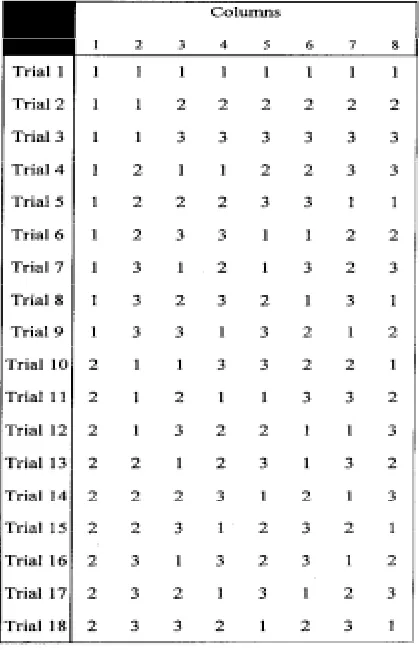
The analysis of important design parameters of cleaning process was being done after brainstorming sessions had taken place with manufacturing, engineering, and quality control persons. The outcome of the sessions gave rise to 8 controllable factors of 2 and 3 levels (Table 2). Since 8 factors were identified and since due to some considerations like costs, time, and impractical conduction of many trials in real production, the decision about the tests of presence of interactions were left to comparing the slopes of
the lines drawn for interaction between factors, and therefore specific interaction were not designed into the experiment, the standard orthogonal array L18 of experimental design was used (Table 3).
Conduction of Experiment and Collection of
Data
The 18 tests of designed experiment were conducted in 9 working days, each in one shift. For each test, 7 random samples of 100 grams were taken and then it was processed through a pilot cleaning machine in laboratory to give the weight percentage of first (A), second (B), third (C), and fourth (D) grade barleycorn content in the sample (Table 4).
6. ANALYSIS OF EXPERIMENT
grade barleycorn to malting process) in this study. One such performance statistic which can reflect the effects of categorized sources of variation (i.e., due to external, internal, and unit to unit variation) is the performance statistic Z(
θ
) given below. For this, the performance characteristic Y which takes non negative values with a target value equal to zero (τ
=0), and a loss function L (Y) which increases as Y increases from zero, reflects the present study. In this case the expected loss, i.e. l(y)=k. E[Y2], is proportional toMean Squared Deviations from Target Value = MSD (
θ
)
= E [(Y-0) 2 ] = E [ Y2 ]. Taguchi recommends using the performance measure)
(
θ
ξ
= - 10 log MSD (θ
).Thus the larger the performance measure, the smaller is the mean squared deviation. Let y1, y2, …, yn approximate a random sample from the distribution of Y for a given design parameters settings (
θ
). The above performance measure can then be estimated by the performance statisticZ (
θ
) = S/N = - 10 log [∑
y
i2/
n
]where the performance statistic Z (
θ
) is themethod of moments estimator of
ξ
(
θ
)
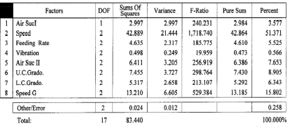
. It is in this context that transformed data of each test in the experiment is calculated and analysis of variance (ANOVA) table is computed (Table 5). From the ANOVA table, it appears that 7 of the 8 considered design parameters with contribution percentage are significant at one percent level of significance (F0.01,1,2 = 98.5 , F0.01,2,2 = 99.0 ) and therefore are able to counteract the effects of the mentioned noise factors on the performance characteristic. The validity of F-test confirmed through satisfactory results achieved from normal probability graph of data and Bartlett test for constant variances.To optimize the settings, the main effects are calculated (Table 6) and then optimum condition and performance are computed (Table 7) through average level estimates of the design parameters. The optimum settings based upon the design parameters are to be A2 B3 C1 D2 E3 F1 G3 H2 and expected result at optimum condition is –9.75 decibel.
Therefore, base upon above findings, the theoretical estimate of expected results from S/N ratio at optimum condition (-9.75) can be calculated as below:
MSD = 10 [-(S/N)/10] = 9.440609
where MSD = [(y1) 2
+ (y2) 2
+ … + (yn) 2
] /n = Mean Squared Deviations from Target Value = Average ( yi)2 = [ E (Y) ]2 or
E (Y) = MSD
T hus, expected performance in QC unit
(Percentage) which is based on S/N = -9.75 at optimum is:
E (Y) = 3.073%
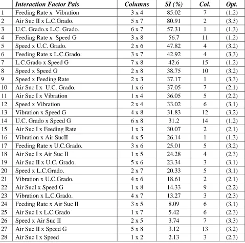
As it is mentioned before, the decision about the presence of interactions can also be made by comparing the slopes of the lines drawn for interaction between factors. The strength of TABLE 8. Interaction Factor Pairs.
Interaction Factor Pais
Columns
SI (%)
Col.
Opt.
1
Feeding Rate x Vibration
3 x 4
85.02
7
(1,2)
2
Air Suc II x L.C.Grado.
5 x 7
80.91
2
(3,3)
3
U.C. Grado.x L.C. Grado.
6 x 7
57.31
1
(1,3)
4
Feeding Rate x Speed G
3 x 8
56.7
11
(1,2)
5
Speed x U.C. Grado.
2 x 6
47.82
4
(3,2)
6
Feeding Rate x L.C.Grado.
3 x 7
42.92
4
(3,3)
7
L.C.Grado x Speed G
7 x 8
42.6
15
(1,2)
8
Speed x Speed G
2 x 8
38.75
10
(3,2)
9
Speed x Feeding Rate
2 x 3
37.17
1
(3,3)
10
Air Suc I x U.C. Grado.
1 x 6
37.05
7
(2,1)
11
Air Suc I x Vibration
1 x 4
36.05
5
(2,2)
12
Speed x Vibration
2 x 4
33.02
6
(3,1)
13
Vibration x Speed G
4 x 8
31.83
12
(3,2)
14
U.C. Grado x Speed G
6 x 8
31.2
14
(1,2)
15
Air Suc I x Feeding Rate
1 x 3
30.07
2
(2,1)
16
Vibration x Air SucII
4 x 5
26.14
1
(1,3)
17
Feeding Rate x U.C.Grado.
3 x 6
25.01
5
(3,2)
18
Air Suc I x Air Suc II
1 x 5
24.28
4
(2,3)
19
Air Suc II x U.C. Grado.
5 x 6
23.34
3
(3,1)
20
Speed x L.C.Grado.
2 x 7
20.33
5
(3,1)
21
Vibration x U.C.Grado.
4 x 6
18.61
2
(2,1)
22
Air SucI x Speed G
1 x 8
14.33
9
(2,2)
23
Vibration x L.C.Grado.
4 x 7
13.27
3
(2,3)
24
Feeding Rate x Air Suc II
3 x 5
8.09
6
(3,1)
25
Air Suc I x L.C.Grado
1 x 7
5.42
6
(2,3)
26
Speed x Air Suc II
2 x 5
3.74
7
(3,3)
27
Air Suc II x Speed G
5 x 8
3.12
13
(3,2)
presence of interaction may be calculated by degrees magnitude at angles of the lines which range between zero, 0o, and ninety, 90o. The term severity index (SI) is defined such that SI = 100% when the angle between the lines is 90o and SI = 0 when the angle is zero [8]. As it can be observed from severity index (SI) of interacting factor pairs (Table 8), the optimum levels of considered factors are almost the same as optimum levels which are obtained through ANOVA of effective factors; and small-observed discrepancies,
which are due to ineffective factors, are negligible. Thus, there would be no need to change any level factors of optimum condition due to interaction effects.
7. CONCLUSION
The theoretical results of this study clearly indicate the reduction of outgoing fourth grade (unwanted) TABLE 9. Confirmation Trail Data under Current and Proposed Conditions.
Sample Under Current Condition Under Proposed Condition
1 A = 9.73 %
C = 38.20 %
B = 30.46 %
D = 21.61 %
A = 30.46 %
C = 22.58 %
B = 42.76 %
D = 4.08 %
2 A = 11.80 %
C = 37.45 %
B = 34.54 %
D = 16.21 %
A = 27.73 %
C = 24.37 %
B = 42.37 %
D = 5.53 %
3 A = 13.01 %
C = 36.51 %
B = 33.05 %
D = 17.43 %
A = 29.73 %
C = 24.24 %
B = 40.11 %
D = 5.92 %
4 A = 19.76 %
C = 29.46 %
B = 36.73 %
D = 14.05 %
A = 32.00 %
C = 22.38 %
B = 40.57 %
D = 5.05 %
5 A = 13.41 %
C = 33.10 %
B = 35.12 %
D = 18.73 %
A = 30.46 %
C = 22.74 %
B = 41.52 %
D = 5.28 %
6 A = 14.91 %
C = 35.29 %
B = 36.82 %
D = 12.98 %
A = 31.29 %
C = 24.41 %
B = 40.80 %
D = 3.50 %
7 A = 12.27 %
C = 35.51 %
B = 33.20 %
D = 19.02 %
A = 30.46 %
C = 22.58 %
B = 42.76 %
D = 4.20 %
Average of Grades Under Current Condition Average of Grades Under Proposed Condition
Grade A = 13.55 %
Grade B = 34.25 %
Grade C = 35.05 %
Grade D = 17.15 %
Grade A = 30.30 %
Grade B = 41.56 %
Grade C = 23.43 %
Grade D = 4.694 %
Descriptive Data of Grade D Under Current Condition Descriptive Data of Grade D Under Improved Condition
Avg. value = 17.147
Std. Dev. = 5.995
Range = 8.63
MSD = 301.719
S/N Ratio = -24.796
Avg. value = 4.794
Std. Dev = 0.88
Range = 2.42
MSD = 23.649
barleycorns of cleaning sub-process into next (malting) sub-process. The results also indicated the mentioned reduction should be around 3.073 percent which is a wonderful outcome as this is to be achieve without imposing any further investment in factors of production. However, in order to support the theoretical achievements, a confirmation trial for proposed optimum condition was planned and its data was obtained (Table 9). The comparison of unwanted incoming fourth grade barleycorns into malting process under current and optimum conditions (Table 9) shows that the fourth grade barleycorns reduced from 17.147 % in current condition to 4.794% in proposed condition which in turn shows a 358%
improvement over the current situation. That is,
% 358 1 % 794 . 4
% 147 . 17
100 1
condition proposed
under
barleycorn grade
fourth of
Percentage
condition nt
undercurra
barleycorn grade
fourth of
Percentage
percent n
conditioni current
over t advancemen Percentage
=
−
=
×
− =
Based on assumed normal performance distribution of quality characteristic and data obtained in confirmation trials, the comparison of normal plots at current and improved conditions may be as indicated in Figure 10.
Apart from major objective of the study, which was reduction of incoming fourth grade barleycorns into malting process, following subordinated results have been also achieved:
1. The average percentages of A and B grade barleycorns have been increased from 13.55 % and 34.25% to 30.30% and 41.56%, respectively. This shows that before conduction of this study, a noticeable percentages of A and B grade barleycorns were led to waste bags and instead the D grade barleycorns were going into malting process.
2. For every 9000 kilos daily processing, 1111.77 kilos of barleycorns can be saved (i.e., 17.147% - 4.794% = 12.353%
⇒
9000 * 12.353% = 1111.77) and therefore cost of processing is diminished and efficiency of cleaning sub-process is increased by 1111.77 kilos for the same two shift working hours.The amount of A and B grade barleycorns,
which was led to waste bags and sold as a waste, now can be led to malting sub-process and cause higher quality and efficiency in malting and next sub-processes.
8. REFRENCES
1. Taguchi, G., “Introduction to Quality Engineering”, Asian Productivity Organization, Distributed by American Supplier Institute Inc., Dearborn, MI, (1986).
2. Phadke, S. M., “Quality Engineering using Robust Design”, Prentice Hall, Englewood Cliffs, N.J, (1989). 3. Gunter, B., “A Perspective on the Taguchi Methods”,
Quality Progress, (June 1987), 44-52.
4. Shoemaker, A. C., Tsui, K. L. and Wu, C. F. J., “Economical Experimentation Methods for Robust Design”, Technometrics, Vol. 33, No. 4, (1991).
5. Kackar Raghu, “ Off–Line Quality Control, Parameter Design, and the Taguchi Method”, Journal of Quality
Technology, Vol. 17, No. 4, (1985), pp.176-188.
6. Bisgaard, S. and Ankenman, B. “ Analytic Parameter Design”, Quality Engineering, Vol. 8, No. 1, (1996), 75-91.
7. Taguchi, G. and Jugulum, R., “The Mahalanobis-Taguchi Strategy: A Pattern Technology System”, New York, Wiley, (2002).