2 DOF H- Infinity Loop Shaping Robust Control for Rocket Attitude Stabilization

2 DOF H- Infinity Loop Shaping Robust Control for

Rocket Attitude Stabilization

Swapnil Pramod Kanade

, Abraham T Mathew

Department of Electrical Engineering, National Institute of Technology, Calicut, 673601, Kerala

Abstract

presence of all uncertainties. Attitude control of rocket is a benchmark proble m in aerospace and missile guidance control because such a system is subjected to number of uncertainties like flight path change, mass variation, thrust variat ion, drag and so on. In this paper the robust control techniques for attitude control of rocket has been e xa mined. The control proble m consists of actuating of fin deflections by the autopilot which mod ifies angle of attack and sideslip angle while stabilizing the rocket rotational mot ion. In order to separate the uncertainties fro m no mina l mode l, the uncertainties are e xpressed as diagonal structure in form of ULFT (Upper Linear Fractional Transforms) which avoids unnecessary conservation. Then 2 DOF H-∞ loop shaping technique is carried out for pitch rate control problem. This has been compared with H-∞ controller design technique. It has been observed that 2 DOF H-∞ loop shaping technique can provides good robust stability and performance. Extensive simulat ions have been carried out to evaluate system performance. The comparat ive results are included in this paper.

Keywords

1. Introduction

Rockets differ fro m a irc raft and spacecraft due to the rapidly time-varying para meters of their equations of motion, which often requires special guidance and control design strategies and short duration of flights. Furthermore, the fast response times required in both translation and rotation of rockets necessitate a much larger control loop bandwidth than that of either an aircra ft or a spacecraft.

With the advancement in control theory, it is now possible to design control system using MIMO fra me work. Also are new mathemat ical approaches that take into account for the modeling uncertainties, disturbance & measurement noise and render a robust controller. New methods have appeared in literature for attitude control of rocket. Fore xa mp le optima l control adaptive control , nuero- fuzzy control, robust control lyapunov based control design and genetic algorith m develop ment. Adaptive technique assures high computation speed.

The rocket should be able to perform some maneuvers. This may inc lude la rger angle of attack, rap id rotational rate change, la rger angular accele rat ion and wide va riat ion in pressure and speed. This makes control proble m challenging th at requ ires gua rant ee ing rob ust stab ilit y and robust

* Corresponding author:

[email protected] (Swapnil Pramod Kanade) Published online at http://journal.sapub.org/aerospace

Copyright © 2013 Scientific & Academic Publishing. All Rights Reserved

performance in p resence of large para meter variat ion andun modelled dynamics with nonlinearities.

In 1981 Za mes[1] brought H-∞ norm as a performance require ment. H-∞ control techniques developed by Doyle et al[2] ,Glover et a l[3] not only offe rs the tradeoff between performance and control effort but also provides the capabili ties of acco mmodating the d isturbance and paramete r variat ion. Re ichert[4] was the first to apply H-∞ control and to show how it advantages over classical control in autopilot design. Simila r autopilot designs were considered byRe iche rt Wise and Jackson. The autopilot robustness uncertain aerodynamic para mete rs are also e xa mined by Wise.

Fro m[11] we see that the H-∞ loop shaping controller was proposed by McFarlane and Glover in 1990. The systematic procedure was developed by Hyde in 1993. After that Limbeer,Kasenally and Perkinns extended it to 2 DOF loop shaping controller development and formulate standard H∞ optimization proble m which a llows to use model matching function in robust stabilization.

In this paper 2 DOF feedback H-∞ loop shaping techniqu es is applied for pitch rate control of roc ket. Applicat ion to rocket model shows that closed loop system for pitch rate control is robust under structural natural frequency variation. In this paper ae rodynamic data which is the function of Mach number 2.78 used for design purpose and the parameters are related to that described in [8]. The controlle r should guaran tee stability for the model in addition to the performance specification that will be de manded.

on 2 describes about system modeling and equations of mot ion, linearizat ion of model, uncertainty modeling. Sect ion 3 includes 2 DOF loop shaping design details. Section 4 contains results, discussion & limitations of two approaches. Section 5 describes conclusion.

2. System Modeling

The model o f rocket is first derived using 6 DOF custom variable mass blocks.

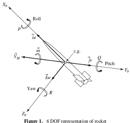
The six degrees of freedo m consist of three translations, and three rotations, along and about the missile ( Xb ,Yb, Zb ) a xes. These motions are illustrated in Figure (1) the translations being (u,v,w) and rotation (P,Q,R) . Following Figure 1 shows complete 6 DOF representation of rocket

Figure 1. 6 DOF representation of rocket

In compact fo rm, the translation and rotation of a rigid body may be e xpressed mathematica lly by the following equations.

Translation: ∑ F=ma Rotation: ∑𝜏𝜏= 𝑑𝑑

𝑑𝑑𝑑𝑑(𝑟𝑟×𝑚𝑚𝑚𝑚)

2.1. Assumptions for Modeling of Rocket & Rocket Model Analysis

No model can be truly depicting its real system. So the model is only appro ximate representation of the behavior of the real system. The model for the rocket is derived based on following assumptions:[6],[9]

1. The rocket equations of motion are written in the body-axes coordinate fra me.

2. A spherical Ea rth rotating at a constant angular velocity is assumed.

3. The vehic le ae rodynamics are nonlinear. 4. The winds are defined with respect to the Earth. 5. An inverse-square gravitational la w is used for the spherical Earth model.

6. The gradients of the low-frequency winds are s mall enough to be neglected.

7. A constant mass will be assumed, that is dm/dt =0 8. The aerodynamic forces and mo ments acting on the vehicle is assumed to be invariant with the position of rocket relative to the free stream velocity vector. Consequently the assumption greatly simp lifies the equation of motion by eliminating the aerodynamic cross coupling terms between roll mot ion and pitch, yaw mot ion. In addition a different set of aerodynamic characteristics for pitch and yaw is not required.

Figure 2. Pitch plane force diagram

In controller design only pitch perturbation motion is considered. In this case rocket attitude is characterized by pitch angle θ and flight path angle Θ or equivalently angle of attack α and θ. Due to rocket symmetry the yaw stabilization system is analogous to pitch stabilizat ion system[7] . Hence equation of motion in p itch plane is considered. The followi ng Figure 2 shows comp lete free body diagra m for pitch plane analysis with mathe matical equations.[8-10].

In following Figure 2 re ference fra me notations used for writ ing equations of motion as the x* -a xis of the vehicle-ca rried vertica l reference fra me is d irected to the North, the y*

-a xis to the East. The x1-a xis of the body-fixed re ference fra me is d irected towards to the nose of the rocket, the y1- a xis points to the top wing. The x-a xis of the flight-path reference fra me is aligned with the velocity vector V of the rocket and the y-a xis lies in the plane x1 y1.

1. Equations describing the motion of the mass centre

𝑚𝑚𝑉𝑉̇=𝑃𝑃𝑐𝑐𝑐𝑐𝑐𝑐𝛼𝛼 − 𝑄𝑄 − 𝐺𝐺𝑐𝑐𝐺𝐺𝐺𝐺𝐺𝐺+𝐹𝐹𝑥𝑥(𝑑𝑑) (1)

𝑚𝑚𝑉𝑉𝐺𝐺̇=𝑃𝑃sin𝛼𝛼+𝑌𝑌–𝐺𝐺𝑐𝑐𝑐𝑐𝑐𝑐𝐺𝐺+𝐹𝐹𝑦𝑦(𝑑𝑑) (2) where

P = engine thrust.

Q = aerodynamic drag.

𝐹𝐹𝑥𝑥(𝑑𝑑),𝐹𝐹𝑦𝑦(𝑑𝑑) = generalized disturbance forces in x, y direction.

m = mass of rocket V = velocity of rocket

2. Equations, describing the rotational motion about the mass centre

𝐼𝐼𝑧𝑧𝜔𝜔𝑧𝑧̇ =𝑀𝑀𝑧𝑧𝑓𝑓+𝑀𝑀𝑧𝑧𝑑𝑑+𝑀𝑀𝑧𝑧𝑐𝑐+𝑀𝑀𝑧𝑧(𝑑𝑑)

wher 𝑀𝑀_𝑧𝑧𝑓𝑓 = the rocket mo ments due to the angle of attack α

𝑀𝑀𝑧𝑧𝑑𝑑 = the aerodynamic mo ments due to pitch rate ωz

𝑀𝑀𝑧𝑧𝑐𝑐= the control mo ments due to fins deflection δz

𝑀𝑀𝑧𝑧(𝑑𝑑) = genera lized d isturbance mo ments about corresponding axes.

𝜃𝜃̇ = p itch rate change

3 Equation giving the relationships between the angles α, θ, Θ

𝛼𝛼=𝐺𝐺 − 𝜃𝜃 (4)

4 Equation giving the normal acceleration

𝐺𝐺𝑦𝑦 =−𝑃𝑃cos_𝐺𝐺𝛼𝛼 −𝑄𝑄sin𝛼𝛼+𝑃𝑃sin_𝐺𝐺𝛼𝛼+𝑌𝑌cos𝛼𝛼 (5)

2.2. Line arization of Equations

In order to obtained a linear controlle r equations (1) – (5) are linearised about trim operating points 𝐺𝐺=𝐺𝐺0, 𝜃𝜃 =

𝜃𝜃0_{,𝛼𝛼=𝛼𝛼}0_,𝜔𝜔

𝑧𝑧 =𝜔𝜔0𝑧𝑧,𝛿𝛿𝑧𝑧=𝛿𝛿0𝑧𝑧 under the assumptions that the variations ∆𝐺𝐺=𝐺𝐺 − 𝐺𝐺0,∆𝜃𝜃=𝜃𝜃 − 𝜃𝜃0, ∆𝛼𝛼=𝛼𝛼 −

𝛼𝛼0_,∆𝜔𝜔

𝑧𝑧=𝜔𝜔𝑧𝑧− 𝜔𝜔0𝑧𝑧,∆𝛿𝛿𝑧𝑧=𝛿𝛿𝑧𝑧− 𝛿𝛿0𝑧𝑧 are suffic iently sma ll. In such a case it is fu lfilled that sinΔα ≈ Δα, cos α ≈ 1.

As a result, the linearised equations of the perturbed motion of the rocket take the form

𝐺𝐺̇=𝑃𝑃_{𝑚𝑚𝑉𝑉}+𝑌𝑌𝛼𝛼𝛼𝛼+𝑌𝑌_{𝑚𝑚𝑉𝑉}𝛿𝛿𝑧𝑧𝛿𝛿𝑧𝑧+ 𝐹𝐹𝑦𝑦(𝑇𝑇) 𝑚𝑚𝑉𝑉 𝜔𝜔̇=𝑀𝑀_𝐽𝐽𝛼𝛼𝑧𝑧 𝑧𝑧 𝛼𝛼+ 𝑀𝑀𝜔𝜔𝑧𝑧 𝑧𝑧 𝐽𝐽𝑧𝑧 𝜔𝜔𝑧𝑧+ 𝑀𝑀𝛿𝛿𝑧𝑧 𝑧𝑧 𝐽𝐽𝑧𝑧 𝛿𝛿𝑧𝑧+ 𝑀𝑀𝑧𝑧(𝑑𝑑) 𝐽𝐽𝑧𝑧 𝜃𝜃̇=𝜔𝜔𝑧𝑧 𝐺𝐺𝑦𝑦 =𝑄𝑄+𝑌𝑌 𝛼𝛼 𝐺𝐺 𝛼𝛼+ 𝑌𝑌𝛿𝛿𝑧𝑧 𝐺𝐺 𝛿𝛿𝑧𝑧

𝛼𝛼=𝜃𝜃 − 𝐺𝐺 (6)

where 𝑌𝑌𝛼𝛼 _=𝑐𝑐 𝑦𝑦𝛼𝛼𝑞𝑞𝑞𝑞 ; 𝑌𝑌𝛿𝛿𝑧𝑧 =𝑐𝑐𝛿𝛿𝑧𝑧𝑦𝑦𝑞𝑞𝑞𝑞 ; 𝑀𝑀𝑧𝑧𝛼𝛼=𝑚𝑚𝑧𝑧𝛼𝛼𝑞𝑞𝑞𝑞𝑞𝑞 ; 𝑀𝑀𝜔𝜔𝑧𝑧 𝑧𝑧=𝑚𝑚 𝜔𝜔𝑧𝑧 𝑧𝑧𝑞𝑞𝑞𝑞𝑞𝑞2

𝑉𝑉 ; 𝑀𝑀𝛿𝛿𝑧𝑧𝑧𝑧 =𝑚𝑚𝛿𝛿𝑧𝑧𝑧𝑧𝛿𝛿𝑧𝑧𝑞𝑞𝑞𝑞𝑞𝑞 equations (6) can be represented as

𝐺𝐺̇=𝑎𝑎𝜃𝜃𝜃𝜃𝛼𝛼+𝑎𝑎𝜃𝜃 𝛿𝛿𝑧𝑧𝛿𝛿𝑧𝑧+𝐹𝐹𝑦𝑦(𝑑𝑑)

𝜃𝜃̈=𝑎𝑎_{𝜃𝜃 𝜃𝜃̇}𝜃𝜃̇+𝑎𝑎𝜃𝜃𝜃𝜃𝛼𝛼+𝑎𝑎𝜃𝜃𝛿𝛿𝑧𝑧𝛿𝛿𝑧𝑧+𝑀𝑀𝑧𝑧(𝑑𝑑)

𝛼𝛼=𝜃𝜃 − 𝐺𝐺

𝐺𝐺𝑦𝑦 =𝑎𝑎𝐺𝐺𝑦𝑦𝛼𝛼𝛼𝛼+𝑎𝑎𝐺𝐺𝑦𝑦𝛿𝛿𝑧𝑧𝛿𝛿𝑧𝑧 (7) where 𝑎𝑎𝐺𝐺𝐺𝐺 =𝑃𝑃+𝑌𝑌 𝛼𝛼 𝑚𝑚𝑉𝑉 ;𝑎𝑎𝜃𝜃 𝛿𝛿𝑧𝑧 = 𝑌𝑌𝛿𝛿𝑧𝑧 𝑚𝑚𝑉𝑉 ;𝑎𝑎𝜃𝜃𝜃𝜃̇ = 𝑀𝑀𝜔𝜔𝑧𝑧 𝑧𝑧 𝐽𝐽𝑧𝑧 ; 𝑎𝑎𝜃𝜃𝜃𝜃 =𝑀𝑀 𝛼𝛼 𝑧𝑧 𝐽𝐽𝑧𝑧 ; 𝑎𝑎𝜃𝜃𝛿𝛿𝑧𝑧 = 𝑀𝑀𝛿𝛿𝑧𝑧_𝑧𝑧 𝐽𝐽𝑧𝑧 ; 𝑎𝑎𝐺𝐺𝑦𝑦𝛼𝛼 = 𝑄𝑄+𝑌𝑌𝛼𝛼 𝐺𝐺 ; 𝑎𝑎𝐺𝐺𝑦𝑦𝛿𝛿𝑧𝑧 = 𝑌𝑌𝛿𝛿𝑧𝑧 𝐺𝐺

In (7) we used the notation

𝐹𝐹𝑦𝑦(𝑑𝑑) =𝐹𝐹_{𝑚𝑚𝑉𝑉}𝑦𝑦(𝑑𝑑) and 𝑀𝑀𝑧𝑧(𝑑𝑑) =𝑀𝑀𝑧𝑧_𝐽𝐽(𝑑𝑑)

Equations (7) are e xtended by the equation describing the rotation of the fins

𝛿𝛿𝑧𝑧̈ + 2𝜉𝜉𝛿𝛿𝑧𝑧𝜔𝜔𝛿𝛿𝑧𝑧𝛿𝛿𝑧𝑧̇ +𝜔𝜔𝛿𝛿𝑧𝑧2𝛿𝛿𝑧𝑧=𝜔𝜔𝛿𝛿𝑧𝑧2𝛿𝛿𝑧𝑧0 (8)

Where 𝛿𝛿_𝑧𝑧0 is the desired angle of fins deflection (the servo actuator reference); 𝜔𝜔_{𝛿𝛿𝑧𝑧} is the natural frequency and

𝜉𝜉𝛿𝛿𝑧𝑧 is the damping coefficient of servo actuator

.

The unperturbed longitudinal motion is described by the equations .

𝑚𝑚𝑉𝑉∗_{̇ =𝑃𝑃cos𝛼𝛼}∗_{− 𝑄𝑄}∗_{− 𝑚𝑚𝑔𝑔}

0sin𝐺𝐺∗ 𝑚𝑚𝑉𝑉∗_{𝐺𝐺̇=𝑃𝑃sin𝛼𝛼}∗_+𝑌𝑌∗_{− 𝑚𝑚𝑔𝑔}

0cos𝐺𝐺∗ 𝐻𝐻̇=𝑉𝑉∗_sin𝐺𝐺∗

𝑚𝑚̇=−𝜇𝜇 where 𝛼𝛼∗_=𝜃𝜃∗_{− 𝐺𝐺}∗ 𝛿𝛿𝑧𝑧∗=−𝑚𝑚𝑧𝑧 𝛼𝛼 𝑚𝑚𝛿𝛿𝑧𝑧_𝑧𝑧𝛼𝛼 ∗ 𝑄𝑄∗_=𝑐𝑐 𝑥𝑥𝑞𝑞𝑞𝑞+𝑐𝑐𝛿𝛿𝑧𝑧𝑥𝑥|𝛿𝛿𝑧𝑧∗|𝑞𝑞𝑞𝑞 𝑌𝑌∗_=𝑐𝑐𝛼𝛼 𝑦𝑦𝛼𝛼∗𝑞𝑞𝑞𝑞+𝑐𝑐𝑦𝑦𝛿𝛿𝑧𝑧𝛿𝛿𝑧𝑧∗𝑞𝑞𝑞𝑞

𝑞𝑞=𝜌𝜌𝑚𝑚₂∗2 ;𝜌𝜌=𝜌𝜌(𝐻𝐻)

𝑐𝑐𝑥𝑥 =𝑐𝑐𝑥𝑥(𝑀𝑀) ; 𝑐𝑐𝛼𝛼𝑦𝑦=𝑐𝑐𝛼𝛼𝑦𝑦(𝑀𝑀) ; 𝑐𝑐𝑦𝑦𝛿𝛿𝑧𝑧 =𝑐𝑐𝑦𝑦𝛿𝛿𝑧𝑧(𝑀𝑀) 𝑀𝑀=𝑉𝑉_𝑎𝑎∗∗ ; 𝑎𝑎∗_=𝑎𝑎∗_(𝐻𝐻) 𝑚𝑚𝑧𝑧𝛼𝛼 =�𝑐𝑐𝑥𝑥+𝑐𝑐 𝛼𝛼 𝑦𝑦�(𝑥𝑥𝐺𝐺− 𝑥𝑥𝐶𝐶) 𝑞𝑞 ; 𝑚𝑚𝛿𝛿𝑧𝑧𝑧𝑧= 𝑐𝑐𝛿𝛿𝑧𝑧 𝑦𝑦(𝑥𝑥𝐺𝐺− 𝑥𝑥𝑅𝑅) 𝑞𝑞

𝜃𝜃∗_=𝜃𝜃∗_{(𝑑𝑑) (9)} In these equations, 𝜃𝜃∗(𝑑𝑑) is the desired time progra m for changing the pitch angle of the vehicle.

2.3. Nominal Model and Stability of Model

A nomina l system model has been obtained using the parameters given in the Table 1. The model is described in form of

𝑥𝑥̇=𝐴𝐴𝑥𝑥(𝑑𝑑) +𝐵𝐵𝐵𝐵(𝑑𝑑)

𝑦𝑦=𝐶𝐶𝑥𝑥(𝑑𝑑) +𝐷𝐷𝐵𝐵(𝑑𝑑)

Here 𝑥𝑥(𝑑𝑑)∈ 𝑅𝑅𝑚𝑚×2 is the state vector 𝐵𝐵(𝑑𝑑) ∈ 𝑅𝑅𝑚𝑚×1 is the input vector 𝑦𝑦(𝑑𝑑)∈ 𝑅𝑅𝑝𝑝×1 is the output vector.

𝐴𝐴= 1 × 104_�

−0.0001 0.0001 0 0

−0.1217 −0.0003 0 0.0286

0 0 0.0212 −2.2500

0 0 0.0001 0

� 𝐵𝐵=� 0 0 22900 0 �

𝐶𝐶= [59.1024 0 0 28.7188]

𝐷𝐷= [0]

For mat rix A , the Eigen values −2 ±𝑗𝑗 34.87 corresponds to stable mode and this pair e xp la ins system slow dynamics behavior. The pair −106 ±𝑗𝑗 106.13 gives the unstable mode and e xpla ins about system fast dynamics.

fully observable. It is require to design 𝐵𝐵(𝑑𝑑) given by

𝐵𝐵(𝑑𝑑) =−𝐾𝐾𝑥𝑥(𝑑𝑑) This will g ive a robust performance.

Table 1. System parameters

Symbol Rocket Parameter Value

L Length of rocket 4.2 m

d Rocket diameter 0.168 m

m Initial rocket mass 96 kg Sa Engine nozzle output section area 0.0204 m2

P0 engine thrust at the sea level 740g N

μ propellant consumption per second 0.7 kg/s

Jx

initial rocket moment of inertia about x axis

14.21 × 10 2 kg M2

Jy

initial rocket moment of inertia

about y axis 7.64 kg M

2

Jz initial rocket moment of inertia

about z axis 7.64 kg M

2

XG initial rocket mass centre coordinate 1.7 m

XC

initial rocket pressure centre

coordinate 1.0 m

xR fins rotation axis coordinate 0.5 m

ωn

natural frequency of the

servo-actuator 236 Hz

ξ servo-actuator damping 0.707

tf duration of the active stage of the

flight 25 s

S Reference area 0.094 m2

2.4. Uncer tainty Modeling

Separation of different uncertain parameters in d iffe rent parts of model and combin ing into one block and forming ULFT is basic principle of uncertainty modeling[12]. For above rocket model ma in variat ion of coefficients of perturb ed motion happens in aerodynamic coeffic ients

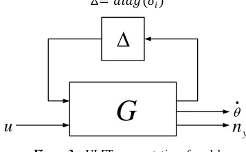
𝑐𝑐𝑥𝑥,𝑐𝑐𝛼𝛼𝑦𝑦,𝑚𝑚𝛼𝛼𝑧𝑧,𝑚𝑚𝑧𝑧𝜔𝜔𝑧𝑧 and these are the function of mach number[7]. For above model 7 coefficients are considered as uncertainty given in equation (7). The uncertainty block △ of all coeffic ients of variation is diagonal matrix of size 7×7. Co mplete ULFT model is shown in Figure 3

△=𝑑𝑑𝐺𝐺𝑎𝑎𝑔𝑔(𝛿𝛿𝐺𝐺)

G

∆

u

n

Figure 3. ULFT representation of model

3. H-

∞ Loop Shaping Design

The loop-shaping design procedure described is based on H ∞ robust stabilization combined with classical loop shapi ng, as proposed by McFarlane and Glover 1992[5].

The open-loop plant is augmented by pre and post-compe nsators to give a desired shape to the singular values of the open-loop frequency response. Then the resulting shaped

plant is robustly stabilized with respect to co prime factor uncertainty using H-∞ optimization. The H-∞ can make a balance between robustness, performance and stability of closed loop system .

3.1. Robust Stabilization Against Nor malize d Coprime Factor Pertur bati ons[11]

To the normal system G constitutes left coprime factorization 𝐺𝐺=𝑀𝑀−1𝑁𝑁. Considering its uncertainty a perturbed model as shown in Figure 4 can be described by

u

_y

∆

∆

N

M

K

φ

Figure 4. Normalized coprime factor uncertainty description

𝐺𝐺= (𝑀𝑀 +∆𝑀𝑀)−1_{(𝑁𝑁+∆𝑁𝑁) (10)}

where ∆𝑀𝑀𝑎𝑎𝐺𝐺𝑑𝑑∆𝑁𝑁 are unknown but stable transfer functions that represent uncertainty in nominal plant model.

The design objective of robust control is to make norma l model G and fa mily of perturbed plant stable. The fa mily of perturbed plant is defined by

𝐺𝐺 = {(𝑀𝑀+∆𝑀𝑀)−1_{(𝑁𝑁+∆𝑁𝑁):‖∆𝑀𝑀,∆𝑁𝑁‖}

∞ <𝜀𝜀} (11) where 𝜀𝜀 is stability marg in. Using sma ll gain theore m the feedback system is robustly stable if (G,K) is internally stable and

�𝐾𝐾(𝐼𝐼 − 𝐺𝐺𝐾𝐾)−1𝑀𝑀−1

(𝐼𝐼 − 𝐺𝐺𝐾𝐾)−1_𝑀𝑀−1 �

∞≤

1

𝜀𝜀 (12)

In order to ma ximize the stability marg in it needed to minimize the 𝛾𝛾=1

𝜀𝜀

𝛾𝛾=��𝐾𝐾_𝐼𝐼�(𝐼𝐼 − 𝐺𝐺𝐾𝐾)−1_𝑀𝑀−1_�

∞ (13) Here γ is the H-∞ norm from ϕ to �𝐵𝐵_𝑦𝑦� and (𝐼𝐼 − 𝐺𝐺𝐾𝐾)−1 is the sensitivity function for this positive feedback arrangement. The lowest achievable va lue of γ and corresponding stability ma rgin 𝜀𝜀 a re given as

𝛾𝛾𝑚𝑚𝐺𝐺𝐺𝐺 =𝜀𝜀𝑚𝑚𝑎𝑎𝑥𝑥−1=�1− ‖[𝑁𝑁 𝑀𝑀]‖𝐻𝐻2� −0.5

= (1 +𝜌𝜌(𝑋𝑋 𝑍𝑍))0.5 ₍₁₄₎

where ‖.‖_𝐻𝐻 denotes the Hankel norm of system 𝜌𝜌 denotes the spectral radius, and for min ima l state space realization of G , Z is unique positive defin ite solution to algebraic Riccati equation

(𝐴𝐴 − 𝐵𝐵𝑞𝑞−1_𝐷𝐷𝑇𝑇_{𝐶𝐶)𝑍𝑍+𝑍𝑍(𝐴𝐴 − 𝐵𝐵𝑞𝑞}−1_𝐷𝐷𝑇𝑇_𝐶𝐶)𝑇𝑇 _{− 𝑍𝑍𝐶𝐶}𝑇𝑇_𝑅𝑅−1_{𝐶𝐶𝑍𝑍+}

𝐵𝐵𝐵𝐵𝑇𝑇_𝑞𝑞−1_{= 0 (15)}

𝑅𝑅 =𝐼𝐼+𝐷𝐷𝐷𝐷𝑇𝑇 _{,𝑞𝑞=𝐼𝐼+𝐷𝐷}𝑇𝑇_𝐷𝐷

X is unique positive definite solution to algebraic Riccati equation

(_{𝐴𝐴 − 𝐵𝐵𝑞𝑞}−1_𝐷𝐷𝑇𝑇_𝐶𝐶)𝑇𝑇_{𝑋𝑋+𝑋𝑋(𝐴𝐴 − 𝐵𝐵𝑞𝑞}−1_𝐷𝐷𝑇𝑇_{𝐶𝐶)− 𝑋𝑋𝐵𝐵}𝑇𝑇_𝑞𝑞−1_{𝐵𝐵𝑋𝑋+}

𝐶𝐶𝑇𝑇_𝑅𝑅−1_{𝐶𝐶= 0 (16)}

A controller which guarantees that

�𝐾𝐾(𝐼𝐼 − 𝐺𝐺𝐾𝐾)−1𝑀𝑀−1

(𝐼𝐼 − 𝐺𝐺𝐾𝐾)−1_𝑀𝑀−1 �

∞≤ 𝛾𝛾 for specified 𝛾𝛾>𝛾𝛾_{𝑚𝑚𝐺𝐺 𝐺𝐺} is given by

𝐾𝐾=�𝐴𝐴+𝐵𝐵𝐹𝐹+𝛾𝛾2(𝑞𝑞𝑇𝑇)−1𝑍𝑍𝐶𝐶𝑇𝑇(𝐶𝐶+𝐷𝐷𝐹𝐹) 𝛾𝛾2(𝑞𝑞𝑇𝑇)−1𝑍𝑍𝐶𝐶𝑇𝑇 𝐵𝐵𝑇𝑇𝑋𝑋 −𝐷𝐷𝑇𝑇 � (17)

where

𝐹𝐹=−𝑞𝑞−1_(𝐷𝐷𝑇𝑇_{𝐶𝐶+𝐵𝐵}𝑇𝑇_{𝑋𝑋) (18)}

𝑞𝑞= (1− 𝛾𝛾2_{)𝐼𝐼+𝑋𝑋 (19)}

3.2. Two Degree of Free dom Controllers[10],[11]

In Doyle et a l. and Limebeer et a l.[5] a t wo degrees-of-fr eedom e xtension of the Glover-McFa rlane procedure was proposed to enhance the model matching properties of the closed-loop . With this the feedback part of the controlle r is designed to meet robust stability and disturbance rejection require ments in a manner similar to the one degree-of-freed om loop-shaping design procedure e xcept that only a pre-co mpensator weight W is used. It is assumed that the measured outputs and the outputs to be controlled are the same althou gh this assumption can be removed as shown later. An additional pre filter part of the controller is then introduced to force the response of the closed-loop system to follo w that of a specified model M called as reference mode l.

3.2.1. Sche me of 2 DOF Control

2 DOF H∞ loop shaping control is a robust controltechni que where the time do main specificat ion can be incorporated in the design. The controllers designed by this approach are

feed-forward pre-filter and feed- back controllers. The feed - forwa rd pre-filter controlle r (K1)is adopted to control the

time do ma in response of the closed loop system, and the feed-back controller is designed for achieving the desired robust stability and the disturbance rejection require ment [10]. In this techn ique, on ly a p re co mpensator we ight func tion (W1) and reference model (Mre f) is needed to be

specified. The shaped plant (Gs) is formulated as the

norma lized co prime factor which separates the nominal plant into normalized nominator & denominator (Ns,Ms)

respectively.

The design problem is to find out stabilizing controller

𝐾𝐾= [ 𝐾𝐾1 𝐾𝐾2] for shaped plant 𝐺𝐺𝑐𝑐 =𝐺𝐺𝑊𝑊1 with norma lized

coprime factorization 𝐺𝐺_𝑐𝑐=𝑀𝑀−1_𝑐𝑐𝑁𝑁_𝑐𝑐 which min imizes the H∞ norm of the transfer function between the signals [𝑟𝑟𝑇𝑇 _𝜙𝜙𝑇𝑇_]𝑇𝑇 _{and [𝐵𝐵}

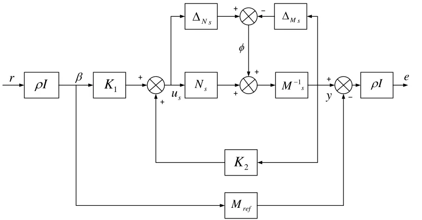
𝑐𝑐𝑇𝑇 𝑦𝑦𝑇𝑇𝑒𝑒𝑇𝑇]𝑇𝑇 as defined in Figure 5. He re 𝜌𝜌 is a scalar va lue specified by the designer to assign the degree of significance of the time do ma in specification.

The control signal 𝐵𝐵_𝑐𝑐 to the shaped plant is given by

𝐵𝐵𝑐𝑐= [𝐾𝐾1 𝐾𝐾2]�𝛽𝛽𝑦𝑦� (20) where K1 is a pre filter and K2 is a feedback controller , β is scaled reference and y is measured output. The purpose of pre filter is to ensure that

�(𝐼𝐼 − 𝐺𝐺𝑐𝑐𝐾𝐾2)−1𝐺𝐺𝑐𝑐𝐾𝐾1− 𝑀𝑀𝑟𝑟𝑒𝑒𝑓𝑓�_∞ ≤ 𝛾𝛾𝜌𝜌−2 (21) Fro m Figure 5 we have

�𝐵𝐵𝑦𝑦𝑐𝑐 𝑒𝑒�=

� 𝜌𝜌(𝐼𝐼 − 𝐾𝐾2𝐺𝐺𝑐𝑐)

−1_𝐾𝐾

1 𝐾𝐾2(𝐼𝐼 − 𝐺𝐺𝑐𝑐𝐾𝐾2)−1𝑀𝑀−1𝑐𝑐

𝜌𝜌(𝐼𝐼 − 𝐺𝐺_𝑐𝑐𝐾𝐾₂)−1_𝐺𝐺

𝑐𝑐𝐾𝐾1 (𝐼𝐼 − 𝐺𝐺𝑐𝑐𝐾𝐾2)−1𝑀𝑀−1𝑐𝑐

𝜌𝜌2[(𝐼𝐼 − 𝐺𝐺𝑐𝑐𝐾𝐾2)−1𝐺𝐺𝑐𝑐𝐾𝐾1− 𝑀𝑀𝑟𝑟𝑒𝑒𝑓𝑓] 𝜌𝜌(𝐼𝐼 − 𝐺𝐺𝑐𝑐𝐾𝐾2)−1𝑀𝑀−1𝑐𝑐

� �_𝜙𝜙�𝑟𝑟 (22)

Here 𝜌𝜌 is a scalar value specified by the designer to assign the degree of significance of the time doma in specification[11].

I

ρ

s N

∆

∆

s

N

M

1

K

2

K

I

ρ

ref

M

r

β

φ

s

u

_y

e

+

+ +

+

+

+ ₋

−

To put the 2 DOF design proble m into the standard control configuration, we can define a generalized plant P by

⎣ ⎢ ⎢ ⎢ ⎡𝐵𝐵_𝑦𝑦𝑐𝑐 𝑒𝑒 𝛽𝛽 𝑦𝑦 ⎦⎥ ⎥ ⎥ ⎤

= �𝑃𝑃11 𝑃𝑃12 𝑃𝑃21 𝑃𝑃22� �

𝑟𝑟 𝜙𝜙 𝐵𝐵𝑐𝑐

� (23)

⎣ ⎢ ⎢ ⎢ ⎡𝐵𝐵_𝑦𝑦𝑐𝑐 𝑒𝑒 𝛽𝛽 𝑦𝑦 ⎦⎥ ⎥ ⎥ ⎤ = ⎣ ⎢ ⎢ ⎢

⎡ 0_{0 𝑀𝑀}0−1 𝐼𝐼

𝑐𝑐 𝐺𝐺𝑐𝑐

−𝜌𝜌2_𝑀𝑀

𝑟𝑟𝑒𝑒𝑓𝑓 𝜌𝜌𝑀𝑀−1𝑐𝑐 𝜌𝜌𝐺𝐺𝑐𝑐

𝜌𝜌𝐼𝐼 0 0

0 𝑀𝑀−1

𝑐𝑐 𝐺𝐺𝑐𝑐 ⎦ ⎥ ⎥ ⎥ ⎤ �𝜙𝜙𝑟𝑟 𝐵𝐵𝑐𝑐

� (24)

Further if the shaped plant Gs and desired stable closed

loop transfer function Mref have the following state space

realizations.

𝐺𝐺𝑐𝑐 =�𝐴𝐴_𝐶𝐶𝑐𝑐 𝐵𝐵𝑐𝑐

𝑐𝑐 𝐷𝐷𝑐𝑐� (25)

𝑀𝑀𝑟𝑟𝑒𝑒𝑓𝑓 =�𝐴𝐴_𝐶𝐶𝑟𝑟 𝐵𝐵𝑟𝑟

𝑟𝑟 𝐷𝐷𝑟𝑟� (26) Then P may be rea lized by

𝑃𝑃= ⎣ ⎢ ⎢ ⎢ ⎢ ⎢ ⎢

⎡ 𝐴𝐴𝑐𝑐 0 0 (𝐵𝐵𝑐𝑐𝐷𝐷𝑐𝑐𝑇𝑇+𝑍𝑍𝑐𝑐𝐶𝐶𝑐𝑐𝑇𝑇)𝑅𝑅𝑐𝑐−0.5 𝐵𝐵𝑐𝑐

0 𝐴𝐴𝑟𝑟 𝐵𝐵𝑟𝑟 0 0

0 0 0 0 𝐼𝐼

𝐶𝐶_𝑐𝑐 0 0 𝑅𝑅_𝑐𝑐0.5 _𝐷𝐷

𝑐𝑐

𝜌𝜌𝐶𝐶_𝑐𝑐 −𝜌𝜌2_𝐶𝐶

𝑟𝑟 −𝜌𝜌2𝐷𝐷𝑟𝑟 𝜌𝜌𝑅𝑅𝑐𝑐0.5 𝜌𝜌𝐷𝐷𝑐𝑐

0 0 𝜌𝜌𝐼𝐼 0 0

𝐶𝐶_𝑐𝑐 0 0 𝑅𝑅_𝑐𝑐0.5 _𝐷𝐷

𝑐𝑐⎦ ⎥ ⎥ ⎥ ⎥ ⎥ ⎥ ⎤ (27)

And used in standard H ∞ algorithm to synthesize controller K. note that Rs and Zs are the unique positive

definite solution to the generalized Riccati equation (15).

3.3. Design Proce dure

The procedure to design 2 DOF H-∞ loop shaping controller as follows[11]:

1. Spec ify the pre -co mpensator we ighting function (W1)

for achieving the desired open loop shape.

2. Specify Mre f which is the desired closed loop transfer

function for time doma in specifications and select 𝜌𝜌 which is a scalar value between 0 and 1. If the designer selects 𝜌𝜌 = 0, the 2DOF H-∞ loop shaping control becomes the 1DOF H-∞ loop shaping control.

3. Find optima l stability margin 𝜀𝜀opt by solving following

equation

𝛾𝛾𝑐𝑐𝑝𝑝𝑑𝑑 =εopt−1

=�� 𝜌𝜌(𝐼𝐼 − 𝐾𝐾2∞𝐺𝐺𝑐𝑐)

−1_𝐾𝐾

1∞ 𝐾𝐾2∞(𝐼𝐼 − 𝐺𝐺𝑐𝑐𝐾𝐾2∞)−1𝑀𝑀−1𝑐𝑐

𝜌𝜌(𝐼𝐼 − 𝐺𝐺𝑐𝑐𝐾𝐾2∞)−1𝐺𝐺𝑐𝑐𝐾𝐾1∞ (𝐼𝐼 − 𝐺𝐺𝑐𝑐𝐾𝐾2∞)−1𝑀𝑀−1𝑐𝑐

𝜌𝜌2[(𝐼𝐼 − 𝐺𝐺𝑐𝑐𝐾𝐾2∞)−1𝐺𝐺𝑐𝑐𝐾𝐾1∞− 𝑀𝑀𝑟𝑟𝑒𝑒𝑓𝑓] 𝜌𝜌(𝐼𝐼 − 𝐺𝐺𝑐𝑐𝐾𝐾2∞)−1𝑀𝑀−1𝑐𝑐

��

∞

4. Select the stability marg in and then synthesize controllers (K1∞,K2∞) that satisfy

‖𝑇𝑇𝑧𝑧𝑧𝑧‖∞

=�� 𝜌𝜌(𝐼𝐼 − 𝐾𝐾2∞𝐺𝐺𝑐𝑐)

−1_𝐾𝐾

1∞ 𝐾𝐾2∞(𝐼𝐼 − 𝐺𝐺𝑐𝑐𝐾𝐾2∞)−1𝑀𝑀−1𝑐𝑐

𝜌𝜌(𝐼𝐼 − 𝐺𝐺𝑐𝑐𝐾𝐾2∞)−1𝐺𝐺𝑐𝑐𝐾𝐾1∞ (𝐼𝐼 − 𝐺𝐺𝑐𝑐𝐾𝐾2∞)−1𝑀𝑀−1𝑐𝑐

𝜌𝜌2_{[(𝐼𝐼 − 𝐺𝐺}

𝑐𝑐𝐾𝐾2∞)−1𝐺𝐺𝑐𝑐𝐾𝐾1∞− 𝑀𝑀𝑟𝑟𝑒𝑒𝑓𝑓] 𝜌𝜌(𝐼𝐼 − 𝐺𝐺𝑐𝑐𝐾𝐾2∞)−1𝑀𝑀−1𝑐𝑐

��

∞ The ele ments (1,1) and (2,1) he lp to limit actuator usage, ele ments (2,2) and (1,2) are associated with robust stability optimization, (3,1) is used to model matching and e le ment (3,2) is linked to the robust performance of the loop.

5. Wi is a scalar vector which is given by

𝑊𝑊𝐺𝐺 =�𝑊𝑊0�−𝐺𝐺𝑐𝑐(0)𝐾𝐾2(0)�

−1

𝐺𝐺𝑐𝑐(0)𝐾𝐾1(0)�

−1

𝑀𝑀𝑟𝑟𝑒𝑒𝑓𝑓(0)

Where

𝑊𝑊𝑐𝑐 =�

1 0 0 0 0 1 0 0 0 0 1 0�

6. Final the feed forward pre filte r and feedback controller (K1 and K2) can be determined by following equation

𝐾𝐾1=𝑊𝑊1𝐾𝐾1∞𝑊𝑊𝐺𝐺

𝐾𝐾2=𝑊𝑊1𝐾𝐾2∞

The schematic diagra m of controlle r is given in following Figure 6. + + 2 K 1 W G 1 K i W Controller r y

Figure 6. 2 DOF H-∞ loop shaping controller diagram

4. Simulation Results and Comparison

of H-

∞ Controller and H-∞ Loop

Shaping Controller Design and

Analysis

4.1. H-∞ Controller Design and Analysis

In our study the rocket parameters are selected fro m Table 1. Figure 7 shows generalized structure of H-∞ controller[13].

r

n

d

u

y

y

y

s

W

u W

p

W

s

e

p

e

u

e

G

)

(

S

K

CONTROLLER

+

−

u

−

M

Figure 7. H-∞ generalized feedback control system

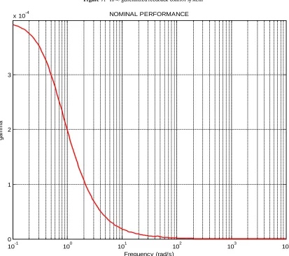
Figure 8. Nominal performance for H-∞ controller

10-1 100 101 102 103 104

0 1 2 3

x 10-4 NOMINAL PERFORMANCE

Frequency (rad/s)

gam

m

The sensitivity we ight function is selected as

𝑊𝑊𝑐𝑐(𝑐𝑐)−1= 0.14�𝑐𝑐

2_{+ 7𝑐𝑐+ 2}

𝑐𝑐2_{+ 4𝑐𝑐+ 9}�

Similarly co mp limentary sensitivity function is selected as

𝑊𝑊𝑝𝑝(𝑐𝑐)−1= 0.6� 𝑐𝑐

2_{+ 4𝑐𝑐+ 8}

𝑐𝑐2_{+ 10𝑐𝑐+ 10}�

The tracking performance weight function Ws is a imed at

minimizing low frequency tracking e rror and the robustness weighting function Wp is to re ject high frequency

mu ltip licat ive uncertainties[14]. In addition the control energy weight function is selected as

𝑊𝑊𝐵𝐵(𝑐𝑐)−1= 0.3�𝑐𝑐

2_{+ 4𝑐𝑐+ 6}

𝑐𝑐2_{+ 7𝑐𝑐+ 9}�

The objective is to avoid actuator operating at high frequencies which lead to saturation[16] . The model matching function is the ideal model to be matched by designed closed loop system wh ich can be selected as[16]

𝑀𝑀 =_{0.0256𝑐𝑐2+ 0.96}1 _{𝑐𝑐+ 1}

The actuator noise weight function chosen as

𝑊𝑊𝐺𝐺 = 0.95 × 10−5�_0.00010.17𝑐𝑐_𝑐𝑐+ 1_{+ 1}�

With above data H-∞ controller is designed. The γ value obtained is 0.1509 which satisfies small ga in theorem[12]. The nominal performance is analyzed and it is 0.00039808 as shown in Figure 8. The frequency response of structured singular values for the case of robust stability is shown in Figure 9. The maximum value of μ is 0.47663 which means that stability of c losed loop system is preserved under all perturbations that satisfy ‖△‖_∞ < 1

0.47663 [12] .The

frequency response of μ for the case of robust performance analysis is given in Figure 10. The peak value of μ is 1.22245 which shows that robust performance has not been achieved.

Figure 11 shows the transient response of closed loop system with designed H-∞ controller for step signal with magnitude 𝑟𝑟= ± 5 which corresponds to change in normal acceleration. The overshoot is 22.74% and settling time is 2.84 sec. The fins deflect ion obtained is 0.1881 rad. ( 11.78°) as shown in Figure 12. The pitch rate variation obtained is 0.1232 (rad/sec) shown in Figure 13 .

Figure 9. μ- Robust stability for H-∞ controller

10-1 100 101 102 103 104

10-9

10-8

10-7

10-6

10-5

10-4

10-3

10-2

10-1

100

robust stability

Frequency (rad/s)

mu

Figure 10. Robust performance for H-∞ controller

Figure 11. Acceleration response for H-∞ controller

100 101 102 103 104

0 0.2 0.4 0.6 0.8 1 1.2 1.4

robust performance

Frequency (rad/s)

mu

upper bound

lower bound

0 1 2 3 4 5 6 7 8 9

-8 -6 -4 -2 0 2 4 6 8

Response in n y

Time (secs) n y

(g

)

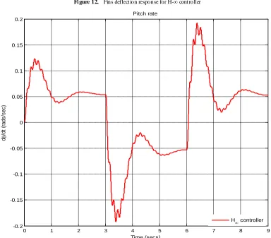
Figure 12. Fins deflection response for H-∞ controller

Figure 13. Pitch rate response for H-∞ controller

0 1 2 3 4 5 6 7 8 9

-0.25 -0.2 -0.15 -0.1 -0.05 0 0.05 0.1 0.15 0.2 0.25

Fins deflection

Time (secs)

δ

(ra

ds

)

H_∞ controller

0 1 2 3 4 5 6 7 8 9

-0.2 -0.15 -0.1 -0.05 0 0.05 0.1 0.15 0.2

Pitch rate

Time (secs)

dθ

/dt

(

rads

/s

ec

)

4.2. H-∞ Loop Shaping Controller Design and Analysis

Here in att itude controller of rocket is designed with 𝐺𝐺_𝑦𝑦 and pitch rate as feedback inputs. The pre compensator W1

selected as

𝑊𝑊1 =�𝑊𝑊₀11 _𝑊𝑊0₂₂�

where

𝑊𝑊11 = 10�16₁₉𝑐𝑐_𝑐𝑐+ 18_{+ 2}�

𝑊𝑊22 = 12�18₁₀𝑞𝑞_𝑞𝑞+ 30_{+ 8}�

Pre co mpensator is always a PI form to have enough slope in the cross frequency while low gain in high frequency can provide enough damping to gain the robustness[17]. The post compensator W2 is selected as

𝑊𝑊2 =�1 0_{0 1}�

where

𝑊𝑊11 = 1 & 𝑊𝑊22 = 1

Post compensator generally re flects the re lative importan ce of outputs to be controlled and therefore it can be chosen as a identity matrix[15]. The diagonal we ight function puts constant weights on control actuators[16].In such a way W1

and W2 are used to modify the nominal system G as W2GW1.

The value of 𝜌𝜌 is taken as 1.The model matching function is selected as

𝑀𝑀 =_{0.0256𝑐𝑐2+ 0.96}1 _{𝑐𝑐+ 1}

Synthesize the controlle r K∞ to make transfer function fro m disturbance to error minimu m. For a ll MIMO systems

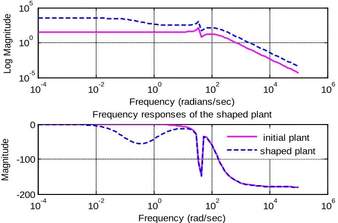
for γ < 4 it can be shown theoretically that controller K∞ does not change shapes of singular values[19]. The robust stability is ach ieved without significant degradation in original characteristics. If γ > 4 then readjust the weight matrix. The controller is synthesized and stability marg in (emax) calculated is 0.40851. The ga mma value obtained is 2.44792 which satisfies stability marg in. Figure 14 shows the frequency response of init ial plant and shaped plant.

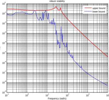
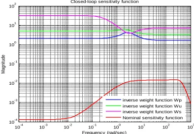
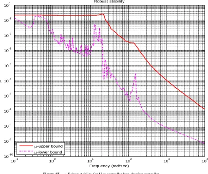
The sensitivity function of the closed loop system is shown in Figure 15. It can be see that require ment of disturbance attenuation is satisfied[18]. The nominal performance is analyzed and it is 0.0053998 as shown in Figure 16. The frequency response of structured singular values for case of robust stability is shown in Figure 17. The maximum value of μ obtained is 0.25883 which means that stability of c losed loop system is preserved under all perturbations that satisfy ‖△‖_∞< 1

0.25883 [12]. The

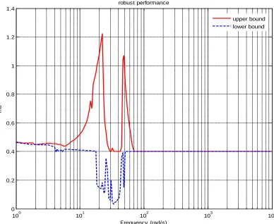
frequency response of μ for the case of robust performance analysis is given in Figure 18. The peak value of μ is 0.41893 which shows that robust performance is ach ieved and in higher frequency range it ma intains constant value.

Figure 19 shows the transient response of the closed loop system with designed 2 DOF H-∞ loop shaping controller for step signal with magnitude 𝑟𝑟= ± 5 which corresponds to change in normal accele ration. The overshoot is found to be 14.72%and corresponding settling time is 2.23 sec. The fins deflection obtained is 0.1617 rad. ( 9.27°) as shown in Figure 20. The pitch rate variation obtained is 0.1 (rad/sec) as shown in Figure 21.

Figure 14. Frequency response of initial plant and shaped plant for H-∞ loop shaping controller

10-4 10-2 100 102 104 106

10-5 100 105

Log M

agni

tude

Frequency (radians/sec)

10-4 10-2 100 102 104 106

-200 -100 0

M

agni

tude

Frequency (rad/sec)

Frequency responses of the shaped plant

Figure 15. Closed loop sensitivity function for H-∞ loop shaping controller

Figure 16. Nominal performance for H-∞ loop shaping controller

10-4 10-3 10-2 10-1 100 101 102 103 10-4

10-3 10-2 10-1 100 101 102

Closed-loop sensitivity function

Frequency (rad/sec)

M

agni

tude

inverse weight function Wp inverse weight function Wu inverse weight function Ws Nominal sensitivity function

10-1 100 101 102 103 104

10-6

10-5

10-4

10-3

10-2

Frequency (rad/sec)

M

agni

tude

Figure 17. μ- Robust stability for H-∞ controller loop shaping controller

Figure 18. Robust performance for H-∞ loop shaping controller

10-1 100 101 102 103 104

10-10

10-9

10-8

10-7

10-6

10-5

10-4

10-3

10-2

10-1

100

Frequency (rad/sec)

µ

Robust stability

µ-upper bound

µ-lower bound

100 101 102 103 104

10-3 10-2 10-1 100

Frequency (rad/sec)

µ

Robust performance

Figure 19. Acceleration response for H-∞ loop shaping controller

Figure 20. Fins deflection response for H-∞ loop shaping controller

0 1 2 3 4 5 6 7 8 9

-8 -6 -4 -2 0 2 4 6 8

Response in n_y

Time (secs)

n y

(g

)

ref.step signal

H_∞ loop shaping controller

0 1 2 3 4 5 6 7 8 9

-0.2 -0.15 -0.1 -0.05 0 0.05 0.1 0.15 0.2

Fins deflection

Time (secs)

δ

(ra

ds

)

Figure 21. Pitch rate response for H-∞ loop shaping controller

4.3. Comparison and Li mitations of Two Appr oaches

The comparison of closed loop system with H-∞ and H-∞ loop shaping controllers begins with robust stability and performance analysis. To achieve robust stability it is neces sary that the μ values are less than 1 over the frequency range. In Figure 22 we co mpare the structured singular values, for the robust stability analysis, of the closed-loop systems with both controllers. It shows that H-∞ loop shaping controller achieving better result.

Table 2. Comparison of 2 controllers parameters

parameters H-∞

controller

H-∞ loop Shaping controller

Nominal performance 0.000398 0.0053998

Robust performance 1.22245 0.41893 μ– robust stability 0.47663 0.25883

Peak overshoot 22.74% 14.72%

Settling time 2.84 Sec 2.23 Sec

Fin deflection 11.78

0

(0.1881 rad)

9.270

(0.1617 rad) RMS value of control

signal 0.195587 0.151148

The co mparison of nominal performance o f t wo controlle rs is shown in Figure 23. In case of H-∞ loop shaping controller performance is slightly more than H-∞ controller. The slightly larger magnitude over the low frequencies leads to an expectation of steady state errors. The robust performance is also computed as shown in Figure 24. It shows that H-∞ loop shaping controller achieves better performance than H-∞ controller in low frequency range.

The output sensitivity to disturbance is less in H-∞ loop shaping approach as shown in Figure 25. Further we can reduce output sensitivity to disturbance by using high gain values in pre filter design. Transient response of controller is shown in Figure 26. The peak overshoot is reduced in H-∞ loop shaping approach also response is less oscillatory but settling time is not reduced to la rge e xtent. As shown in Figure 27 fins deflection is reduced it shows longitudinal stability is imp roved in H-∞ loop shaping approach. Reduction in pitch rate is also achieved by H- ∞ loop shaping controller as shown in Figure 28. The RMS va lue of control signal related to fuel consumption. As value decreases proportionally fue l consumption reduced. RMS value is less in H-∞ loop shaping approach so using H-∞ loop shaping controller fuel consumption reduced. Table 2 shows comparison of performance para meters of two controllers.

Figure (22) to (28) shows comparison of parameters of 2 controllers

0 1 2 3 4 5 6 7 8 9

-0.2 -0.15 -0.1 -0.05 0 0.05 0.1 0.15

Pitch rate

Time (secs) dθ

/dt

(

rads

/s

ec

)

Figure 22. μ- Robust stability for both H-∞ and H-∞ loop shaping controller

Figure 23. Nominal performance of H-∞ and H-∞ loop shaping controller

10-3 10-2 10-1 100 101 102 103 104

10-6 10-5 10-4 10-3 10-2 10-1 100

Robust stability for all controllers

Frequency (rad/s)

U

pper

bound of

µ

H_∞ controller

loop shaping controller

10-2 10-1 100 101 102 103 104

10-12 10-10 10-8 10-6 10-4 10-2

Frequency (rad/sec)

M

agni

tude

Nominal performance of controllers

H_∞ controller

Figure 24. Robust performance for H-∞ and H-∞ loop shaping controller

Figure 25. Output sensitivity for H-∞ and H-∞ loop shaping controller

100 101 102 103 104

0 0.2 0.4 0.6 0.8 1 1.2 1.4

Frequency (rad/sec)

U

pper

bound of

µ

Robust performance for controllers

H_∞ controller H_∞ controller

Loop shaping controller

10-2 10-1 100 101 102 103 104

-160 -140 -120 -100 -80 -60 -40 -20 0 20

Frequency (Hz)

M

agni

tude (

dB

)

Output sensitivity to disturbance

H_∞ controller

Figure 26. Response for acceleration for H-∞ and H-∞ loop shaping controller

Figure 27. Response for fins deflection for H-∞ and H-∞ loop shaping controller

0 1 2 3 4 5 6 7 8 9

-8 -6 -4 -2 0 2 4 6 8

Response in n y

Time (secs)

n y

(g

)

ref.step signal H_∞ controller

H_∞ controller loop shaping

0 1 2 3 4 5 6 7 8 9

-0.25 -0.2 -0.15 -0.1 -0.05 0 0.05 0.1 0.15 0.2 0.25

Fins deflection

Time (secs)

δ

(ra

d

s

)

H_∞ controller

Figure 28. Pitch rate for both H-∞ and H-∞ loop shaping controller

Figure 29. Acceleration response due to 5% decrement parameters

0 1 2 3 4 5 6 7 8 9

-0.2 -0.15 -0.1 -0.05 0 0.05 0.1 0.15 0.2

Pitch rate

Time (secs)

dθ

/dt

(

rads

/s

ec

)

H_∞ controller

H_∞ controller loop shaping

0 1 2 3 4 5 6 7 8 9

-5 -4 -3 -2 -1 0 1 2 3 4 5

Response in n_y ( Due to 5% decrement in system parameters )

Time (secs)

n y

(g

)

ref.step signal H_∞ controller

Figure 30. Acceleration response due to 5% increment parameters

In above discussion controllers a re designed and compare d their performance results. Every controller has its specific operating range and depends upon system para meter variati on. In above system 5 % change in system para meters ,the controller fa ils. Table 3 shows peak over shoot. The responses are shown in Figure 28 and 29.

Table 3. Effect on change in peak overshoot

% change in parameters

Peak overshoot

H-∞ controller H-∞ loop shaping _controller

5 % increment 240% 180%

5 % decrement -196% -160%

Fro m above table it shows peak overshoot exceeds it ma ximu m limit. So fo r our controller we can vary system parameters up to 1% obtaining desired value in range .

5. Conclusions

A rocket model is developed in which pitch rate control is analyzed and simu lated. The pitch rate control proble m is related to the longitudinal stability of the rocket. According to result obtained from simu lation it can be seen that longitu dinal stability is improved using 2 DOF loop shaping controller.

Due to presence of uncertain parameters the derivation of the uncertainty model required and heavy computations are demanded. That is the main reason why it is necessary to investigate the parameter importance with respect to the robustness performance and an objective is to reduce their number to an acceptable value. However, in the evaluation of

the design, it is better to take into account all the possible uncertainties to ensure a satisfactory design in a present case. Here 15% uncertainties in para mete rs are taken.

The performance of closed loop system using H-∞ loop controller is evaluated .The model facilitates γ iteration method for solving Ricatti equation for H-∞ controller design The performance of the c losed loop system using H-∞ loop shaping controller is further evaluated. The application of a 2 DOF H- ∞ loop shaping controller in pitch rate auto pilot design shows that it is better in robustness and reduces control efforts without the degrading performance.

Actuator efforts are critica l consideration in the rocket auto pilot design since they invoke how quickly actuator command limit ing is invoked. The pitch rate reduced and reduction in fins deflection shows that actuator efforts are reduced.

Nomenclature

Symbol Meaning

ϑ Pitch Angle

ψ Yaw Angle

γ Roll Angle

α Angle Of Attack

β Sideslip Angle

Θ Flight-Path Angle

Ψ Bank Angle

γc Aerodynamic Angle Of Roll

δy, δz

Angles Due To Fins Deflection In Longitudinal And Lateral Motion

M Mach Number

0 1 2 3 4 5 6 7 8 9

-25 -20 -15 -10 -5 0 5 10 15 20 25

Response in n_y ( Due to 5% increment in system parameters )

Time (secs)

n y

(g

)

ref.step signal H_∞ controller

REFERENCES

[1] Zames G.(1981) “Feedback and optimal sensitivity model reference transformation, multiplicative semi norms and approximate references.” IEEE Transaction On Automatic Control AC-23 (1981), 301-302

[2] Doyle J., Glover K, Khargoeker P., and Fracis B (1989) “State space solution to standard H2 and H∞ control problem ” IEEE Transaction On Automatic Control 34 (1989), 831-847 [3] Glover k, Limebeer D, Doyle j, Kasenally E.M , and Sofonov

M , (1991) “A characterization of all solutions to four block distance problem” SIAM Journal of control and optimization , 29 (1991) 283-324

[4] Reichert R T (1989) “Application of H_∞ control to missile autopilot design” In Proceedings Of AIAA Guidance , Navigation And Control Conference , 1989 1065-1072 [5] M cFarlane, D.C., and K. Glover, "A Loop Shaping Design

Procedure using Synthesis," IEEE Transactions on Automatic Control, vol. 37, no. 6, pp. 759– 769, June 1992.

[6] George m. Siouris “M odern missile guidance and control” springer – verlag .2004 (e-book)

[7] Brodsky, S.A.; Aro, H.O (2011) “Application of robust control for attitude stabilization of supersonic winged rocket”

IEEE Transaction On Control System, 978 – 1 – 4244 – 9616 - 7/11,2011

[8] J.Blaklock “ Automatic control of Aircraft & missiles ”. John wiley & sons. 2004

[9] Jack E. Nelsen “M issile Aerodynamics” Mc Graw Hill Publications 1960

[10] D.W.Gu , P. Peter “Robust control engineering design with MATLAB” .springer – verlag, 2005 1st Edition

[11] S.Skogested, I.Postlethwaite “M ultivariable feedback control system ” wiley & sons .2001

[12] M Green “Linear robust control” chapter 6: Full information

about H-∞ synthesis. Dover publication .1998

[13] M ark .R. Tucker.and Daniel Walker.” H-∞ mixed sensitivity “, Robust flight control- Design challenge, leacture notes in control and information science, Springer- Verlag 2000 [14] Yang S M and Huang H “ Application of H-∞ control to

missile auto pilot design” IEEE transaction on Control system 0018-9251/03

[15] R. Sobhani “ Nonlinear Digital Robust controller for UAV”,

IEEE Aerospace conference 1-4144-0525-4/2007

[16] Sun Jie, Yang Jun “ Robust flight control law development for Tiltrotor conversion” IEEE 2009 International conference on intelligent human machine system and cybernetics 978/0-7695-3753-8/09

[17] M ingyun L V, Yanpenh Hu” Attitude control of unmanned helicopter using H-∞ loop shaping method” IEEE Transaction on Mechatronics sciences 978 – 1 – 61284 – 722 - 1/11 ,2011

[18] J.Gadewadikar, F.L.Lewis, Kamesh Subbarao and Ben M . Chen. “Structured H∞ Command and Control-Loop Design for Unmanned UAV”. Journal Of Guidance, Control, And Dynamics. Vol. 31. No. 4, July-August 2009.

[19] J. Gadewadikar, F. L. Lewis, Kamesh Subbarao and Ben M .Chen.Attitude “Control System Design for Unmanned Aerial Vehicles using H-∞ and Loop-shaping Methods.” 2007 IEEE International Conference on Control and Automation. Guangzhou, CHINA M ay 30 to June 1,2007.

[20] K Glover and R Hyde “H-∞ Loop shaping design for Flight”, Chapter 29 Robust flight control- Design challenge, lecture notes in control and information science, Springer- Verlag 2000