Distance models for analysis of multivariate binary data

(1)

Cover Page

The following handle holds various files of this Leiden University dissertation:

http://hdl.handle.net/1887/67140

Author

: Worku, H.M.

Title:

Distance models for analysis of multivariate binary data

(2)

Invitation

to attend the defense

of the thesis

Distance Models

for Analysis of

Multivariate Binary

Data

on Thursday 20 December

2018 at 3.00 pm in

the Academiegebouw of

Leiden University,

Rapenburg 73 in Leiden

Paranymphs:

Maarten Kampert

&

Yinebeb Tessema

Hailemichael Metiku Worku

Distance Models

for Analysis of

M u l t i v a r i a t e

B i n a r y D a t a

Hailemichael Metiku Worku

Distance Models for Analysis of Multivariate Binary Data

(3)

(4)

Distance Models for Analysis of

(5)

Printed by Ridderprint BV

All rights reserved. No part of this book may be reproduced, stored in a retrieval system, or transmitted, in any form or by any means, electronically, mechanically, by photocopy, by recoding, or otherwise, without prior written permission from the author.

(6)

Distance Models for Analysis of

Multivariate Binary Data

PROEFSCHRIFT

ter verkrijging van de graad van doctor aan de Universiteit Leiden, op gezag van de Rector Magnificus, prof. mr. C. J. J. M. Stolker,

volgens besluit van het College voor Promoties te verdedigen op donderdag 20 december 2018

klokke 15.00 uur

(7)

prof. dr. M. de Rooij prof. dr. W. J. Heiser

Promotiecommissie:

prof. dr. C.J.F. ter Braak (Wageningen University & Research) prof. dr. P. Spinhoven (Leiden University FSW)

prof. dr. S. le Cessie (Leiden University Medical Center) Dr. W. Bergsma (London School of Economics)

Acknowledgement:

(8)

Motto

7_{Though your beginnings were modest, your latter days will be full of}

prosperity. (Job 8:7)

(13)

(14)

Research Articles

As presented below, the chapters of this dissertation are based on published (or to be submitted) articles.

• Chapter 3: Worku, H. M. & De Rooij, M. (2017). Properties of Ideal Point Classi-fication Models for Bivariate Binary Data. Psychometrika,82(2), 308-328.

• Chapter 4: Worku, H. M. & De Rooij, M. (2018). A Multivariate Logistic Distance Model for the Analysis of Multiple Binary Responses. Journal of Classification,35, 1-23. https://doi.org/10.1007/s00357-018-9251-4

• Chapter 5: Worku, H. M. & De Rooij, M.mldm: An R package for Analyzing

Multi-variate Binary Data. The package can be retrieved from https://github.com/workuhm1/mldm-package-github.

(15)

(16)

List of Figures

1.1 MDS Model: A two-dimensional configuration of dissimilarity data with five objects (i.e.,A, B, C, D andE). . . 8 1.2 MDU Model: A two-dimensional configuration of preference data with

four subjects (i.e.,s1, s2, s3 ands4) and five objects (i.e., A, B, C, DandE). . . 9 1.3 A path diagram of a CFA with six indicator variables represented by a

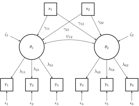
square, and two latent variables represented by a circle. . . 21 1.4 A path diagram for a MIMIC model with two external variables that are

represented by a square. . . 24 2.1 A path diagram of a factor model with six indicator variables represented

by a square, and two latent variables represented by a circle. . . 34 2.2 A path diagram for a MIMIC model with two external variables that are

represented by a square. . . 34 2.3 Interaction plot for Nonconvergence rate: The first three panels (from left

to right) show interaction plot between the type of indicators and the num-ber of indicators, the factor structure, and the sample size, respectively. The last panel is for the interaction between the number of indicators and the sample size. . . 42

(17)

2.4 Interaction plot for Heywood rate: The first four panels (from left to right) show the interaction between the type of indicators and the number of in-dicators, the factor structure, the correlation between underlying latents, and the sample size, respectively. The last two panels are for the inter-action between the number of indicators and the factor structure and the sample size. . . 45 2.5 Interaction plot for Quality of Recovering Factors: The first panel shows

two main effects for the type and number of indicators. The second panel shows the interaction between the type of indicators and the factor structure. 48 3.1 Biplot of the final BIPC model fitted on the NESDA data. The predictors

neuroticism, represented byN; extraversion, byE; and education, byEDU. The bivariate binary responses are dysthmia, represented by DYST; and generalized anxiety disorder, byGAD. The class coordinates that correspond to the multinomial response variable, denoted byG, are also displayed. . . 84 4.1 Biplot of the final “distress-fear” model fitted on the NESDA data, where

the first dimension is represented by three disorders (MDD, GAD and DYST) and the second dimension by two disorders (SP and PD). The plot is based on restrictions applied on the class points. . . 109 4.2 Representation of the binary response variables in the Euclidean space. . 110 4.3 Variable axes representation of the predictor variables (i.e., N:

Neuroti-cism, E: Extraversion, C: Conscientiousness, and EDU: EDUcation) in the Euclidean space. . . 111 5.1 Reading the NESDA data available in themldmpackage. . . 124 5.2 Excerpt of the NESDA data that shows records belonging to the first two

(18)

LIST OF FIGURES xv 5.3 Specification of an indicator matrix for the depression-anxiety model fitted

on the NESDA data. . . 126

5.4 A two-dimensional representation of model formula for depression-anxiety model fitted on the NESDA data. . . 127

5.5 Application of the mldm.fit function for fitting the depression-anxiety model on the NESDA data. . . 128

5.6 Summary of the depression-anxiety model fitted on the NESDA data. . . 131

5.7 Application of the Clustered Bootstrap method with the MLD model. . . 132

5.8 Summary of the depression-anxiety model fitted on the NESDA data using the Clustered Bootstrap method. . . 134

5.9 Application of thebiplot()function available in themldmpackage. . . 135

5.10 The biplot for depression-anxiety model fitted on the NESDA data. . . 135

5.11 Specification of an indicator matrix for candidate models with respect to dimensionality in the model. . . 137

5.12 Specification of model formula for a unidimensional MLD model. . . 137

5.13 Model selection in MLD model for dimensionality. . . 138

5.14 Model formula structure of the candidate MLD models. . . 139

5.15 Model selection in MLD model for explanatory variables. . . 140

(19)

(20)

List of Tables

1.1 The structure of multivariate data in long format. . . 16 1.2 Cross-classification of measurements of a bivariate binary data observed

on thei-th subject. . . 17 2.1 Classes of Latent Variable Models. . . 28 2.2 The design variables with their corresponding values (or ranges) that are

considered in the Monte Carlo simulation study. BLR stands for Binary indicator variables with Low success Rates; and BMR for Binary indicator variables with Moderate success Rates. . . 35 2.3 Percentage of nonconvergence in CFA under different experimental

set-tings. Each cell result is based onR= 100simulated replications. . . 40 2.4 Percentage ofHeywood cases in CFA under different experimental settings.

Each cell result is based onR= 100simulated replications. . . 44 2.5 Quality of Recovering the True Factor scores: Average correlation between

the true and estimated factor scores of CFA, i.e., Corr(θ1,θˆ1) = ˆρ1, under

different experimental settings. Each cell represents the results ofR= 100

simulated replications, except those models that were not identified due to improper solutions. . . 47

(21)

2.6 Observed type-I error rates for the relationship betweenX3 and the first

factor,γ31. The values in bold represent95%confidence interval excluding

the nominal level of significance (α= 0.05). The number of replications per cell differs because of improper solutions. Dashed lines indicate no valid results were obtained for that cell. . . 49 2.7 Observed power for the relationship betweenX5and the first factor,γ51=

−0.30. The number of replications per cell differ because of improper solutions. Dashed lines indicate no valid results were obtained for that cell. 51 3.1 Cross-classification of bivariate binary data observed fromi-th subject. . . 58 3.2 Summarized results of the simulation study for studying the performance

of the IPC model for analysing bivariate binary data. IPC(2D-FIXED) cor-responds to the 2-dimensional IPC model withfixed class points, i.e.,φ1=

φ2= 0;IPC(3D)to the 3-dimensional IPC model; andIPC(2D-FREE)to

the 2-dimensional IPC model withfree class points. . . 73 3.3 Summarized results of the simulation study for studying the performance

of the BIPC model for analysing bivariate binary data. . . 78 3.4 Parameter estimates with corresponding standard errors (between the

paren-thesis) obtained from the IPC and BIPC models fitted on the NESDA data. IPC(2D-IND) corresponds to the 2-dimensional IPC model with

fixed class coordinates; IPC(2D-FREE) to the 2-dimensional IPC model withfree class coordinates; andIPC(3D)to the 3-dimensional IPC model. 79 4.1 The structure of multivariate data in long format. . . 97 4.2 Results of fitting different MLD models to NESDA data. In the first block,

(22)

LIST OF TABLES xix 4.3 Summarized results of the final “distress-fear” MLD model fitted on NESDA

data. Restriction was applied on the class points, and thus it is a restricted MLD model. The reported standard errors are based on both sandwich and clustered bootstrap methods. The number of bootstraps,B= 1000. 108 4.4 Regression weights of the final unrestricted “distress-fear” MLD model

fitted on NESDA data. The number of bootstraps used to obtain standard errors equals1000. . . 113 A.1 Parameter estimates of the 2-way interaction logistic regression model

fitted on the nonconvergence data. For simplicity, we denote the design variables as, a: type of indicators; b: number of indicators; c: factor struc-ture; d: correlation between underlying latent variables; and, e: sample size. . . 149 A.2 Parameter estimates of the 2-way interaction logistic regression model

fitted on theHeywood data. For simplicity, we denote the design variables as, a: type of indicators; b: number of indicators; c: factor structure; d: correlation between underlying latent variables; and, e: sample size. . . . 152 A.3 Effect size of the 2-way interaction ANOVA model fitted on the average

correlations reported in Table 2.5. The design variables are denoted by letters, i.e., a: type of indicators; b: number of indicators; c: factor structure; d: correlation between latent variables; and e: sample size. . . 154 A.4 Observed power for the relationship between X7 and the second factor,

γ72= 0.10. The number of replications per cell differ because of improper

solutions. Dashed lines indicate no valid results were obtained for that cell. 155 A.5 Observed power for the relationship between X4 and the second factor,

γ42= 0.95. The number of replications per cell differ because of improper

(23)

C.1 Fit statistics for the factor models fitted on the NESDA data. . . 160 C.2 Parameter estimates with the corresponding standard errors (S.E.)

(24)

Chapter 1 Introduction

1.1 Categorical Response Data

In statistical analysis, we often explore and analyze a single variable or many variables depending on the research question at hand. A variable, sometimes referred to as a random variable, is a statistical quantity which can be measured or observed. The fol-lowing are examples of a variable: age, gender, survival of a patient (i.e., survived or not survived), mental status (i.e., normal, mild, moderate, severe), marital status (single, married, divorced, widowed), temperature and humidity, carbon emission, etc.

As described by Agresti (2002, Chap. 1), a variable can be classified in different ways: (1) response (sometimes referred to as dependent or outcome) variable versus explanatory (sometimes referred to as independent or predictor) variable; (2) continuous variable versus discrete variable; (3) quantitative variable versus qualitative variable; and, (4) nominal variable versus ordinal variable. Except for the first classification, the criteria for the other classifications are based on the type of values or measurements a variable could take. Gender, for example, is a nominal variable because it takes a value which is either male or female. Gender is also a qualitative variable. Mental status, on the other hand, could be defined either as qualitative or quantitative depending on the research.

(25)

In the above example, mental status is defined as an ordinal qualitative variable since there is a natural ordering between values for severity of mental status. Both survival of a patient and marital status, in the above example, are nominal qualitative variables. Qualitative variables are sometimes referred to as categorical variables. Age, like mental status, could be defined either as a discrete quantitative variable (e.g.,Age (in years) = 23, 24, 43, etc) or as a continuous quantitative variable (e.g.,Age (in hours) = 1.5, 3.5, 8.0, etc) or as a ordinal qualitative variable (e.g.,Age = young, middle, elderly). The other variables in the above example (i.e., temperature, humidity and carbon emission) are defined most of the time as continuous quantitative variables.

In regression analysis or Analysis of Variance (ANOVA), for example, we study the relationship between a response variable and one or more explanatory variable(s). The aim of such analysis is to understand the amount of change on a response variable when a explanatory variable changes by some amount (usually a unit change). For example, a researcher might be interested in the relationship between mental status and age. The hypothesis of her research could be that severity of mental status of a subject might be affected by age. In this case, the response variable is mental status and the explanatory variable is age. Another example where a response variable is continuous, is the relation-ship between level of temperature in a given area (or country) and the amount of carbon emission. In this case, the response variable is temperature and it is a continuous variable. Carbon emission is the explanatory variable since it has the potential to explain level of atmospheric temperature.

(26)

1.2. EXPLANATORY VARIABLES 3

1.1.1 Binary Response Data

A binary response variable is a categorical variable whose values are binary (i.e., yes or no; 1 or 0; survived or not survived; passed or failed). In many areas of research binary response variables are collected. A clinical psychologist might be interested depression,

depression=1 if a given subject in the study has a depression, otherwisedepression=0 representing absence of depression. A cardiologist might be interested to predict the chance of a patient to survive after performing heart surgery (i.e., survival = 1 if a patient survived;survival= 0 otherwise).

1.1.2 Multicategory Response Data

A multicategory response variable is a categorical variable with more than two possible values. Mental and marital status are examples of multicategory response variable.

1.2 Explanatory variables

An explanatory variable is expected to influence the response variable of interest. A possible set of explanatory variables for mental status could be age, residence (i.e., rural or urban), life style (e.g., smoking status, physical exercise, etc), personality traits (e.g., neuroticism, extroversion), etc. In this dissertation the explanatory variables might be continuous or categorical.

1.3 Logistic Regression Model

(27)

cat-egorical response variables, i.e., both binary and multicatcat-egorical variables). Our main focus in this thesis will be GLM for categorical response data.

A GLM has three parts: (1) a random component; (2) a systematic component; and, (3) a link function. The random component represents the distribution of the response variable. The systematic component represents a linear combination of the explanatory variables. The link function is the part which does the linking between the response and the explanatory variables. Below is the mathematical representation of GLM:

g(µ) =β0+β1x1+β2x2+. . .+βkxp, (1.1)

whereµ=E(Y)is the random component and it is the expected value of the distribution of response variable Y from the exponential family. The right-hand side of Eq. (1.1) represents the systematic part of GLM including the intercept (i.e.,β0) and the regression

coefficients (i.e., β1, β2, . . . , βp corresponding to thepexplanatory variables denoted by x). The link function isg(.)and it connects the random part (i.e., µ) to the systematic part (i.e.,β0+βTx, where x= (x1, x2, . . . , xp)T).

1.3.1 Binary Logistic Regression

Binary logistic regression, sometimes referred to as simple logistic regression, is a GLM for binary response data (Agresti, 2007, chap. 4). Let yi denote the observed value of a

binary dependent variableY for subjecti, wherei= 1,2, . . . , N. Binary logistic regression models the probability of a “success” category conditional on the value of explanatory variablesxi,Pr(yi= 1|xi) =π(xi), i.e.,

π(xi) =

exp(β0+βTxi)

1 + exp(β0+βTxi)

, (1.2)

(28)

1.3. LOGISTIC REGRESSION MODEL 5 The log-odds representation of the same binary LR model (1.2) is,

logit[π(xi)] =β0+βTxi, (1.3)

where logit[π(xi)] = log [π(xi)/(1−π(xi))]. This representation of binary LR is similar

to the Generalized Linear model presented in Eq. (1.1) where the link function is now the “logit” function withµ=π(xi) = Pr(yi= 1|xi).

1.3.2 Multinomial Logistic Regression

Multinomial LR model is a GLM for multicategory response data (Agresti, 2007, chap. 6). Let Gi =k denote the observed value of a multicategory dependent variable Gfor

subjecti, wherei= 1,2, . . . , N.

The Multinomial Baseline-Category Logit (MBCL) model is a natural extension of binary logistic regression model to the case of a nominal categorical variable. The prob-ability of the k-th category in MBCL model (i.e., Pr(Gi = k|xi) = πk(xi)) is defined

as,

πk(xi) =

exp(β0k+βkTxi) P

cexp(β0c+βTcxi)

. (1.4)

The log-odds representation of the MBCL model (1.4) becomes,

logit[πk(xi)] =β0k+βkTxik, (1.5)

where logit[πk(xi)] = log [πk(xi)/πb(xi)]. The indexbrefers to the reference (or baseline)

category against which other categories are compared with. Thus, there are (C−1) number of “logit” models in MBCL for a multicategory response variable,G, withC the number of categories.

(29)

location) to spend their weekend. The possible values of the response variableGcould be:

stay at home,meet friends at their place,meet friends at a city center,travel to somewhere

(e.g., park, beach, museum, other cities), and go to the gym. Let Gi = 0,1,2,3,4 be

the numerical representation of the possible values and to be used in the MBCL model, respectively. Suppose the main aim of the investigation is to estimate the probability of preference of people to spend the weekend out of their home. That is, the probability of going to the gym, the park, the beach, museum, and other cities. In this case, the reference/baseline category will be staying at home (i.e.,Gi= 0).

1.3.3 Parameter Estimation in Logistic Regression Models

In logistic regression, parameters of the model (i.e., the intercept and the regression coefficients) are unknown and thus estimated from sample data. Maximum likelihood optimization is a standard method used for estimating the parameters of LR models.

The likelihood function is the probability of the sample data, expressed as a function of model parameters (Agresti, 2002, pp. 6). The likelihood function for a binary LR model assuming a binomial distribution is defined as (Agresti, 2002),

L(y|β) =

N Y

i=1

ni! yi!(ni−yi)

π(xi)yi[1−π(xi)yi]ni−yi, (1.6)

whereni represents the number of trials andyi represents the number of successes, and

β is a concatenation of the intercept and the regression coefficients of the binary LR model. The maximum likelihood estimation technique optimizes the likelihood function (Eq. (1.6)). Similarly, the likelihood function of MBCL model is defined as (Agresti, 2002),

L(G|β) =

N Y

i=1

" ni! Q

cGic! Y

c

πc(xi)Gic #

(30)

1.4. DISTANCE MODELS 7

1.4 Distance Models

Multidimensional scaling (MDS) is a technique developed in the behavioral and social sciences for studying the structure of objects or people (Davison, 1983, pp. 1). MDS uses proximity between pairs of objects as an input for analysis.

The proximity data is either similarity or dissimilarity of objects. In similarity data, the higher value for the proximity measure represents more alike pairs of objects whereas in dissimilarity data, the higher value for proximity measure represents less alike pairs of objects. An example of the latter type of proximities would be flight times.

Other examples of proximity measures are the correlation coefficient and joint prob-abilities (Davison, 1983, pp. 1). We will show later in this thesis that it is possible to express logistic regression models (i.e., Eq. (1.2) and (1.4)) in terms of distance models. In that case, probability is a similarity measure. That is, the smaller the relative distance between a subject (or person) point and a category point, the larger the probability that the subject chooses that category.

1.4.1 Multidimensional Scaling

In MDS, the proximities are represented in terms of distances between points in a low dimensional space (Kruskal & Wish, 1978; Davison, 1983; Borg & Groenen, 2005). The Euclidean distance model for dissimilarity measures is defined as (Davison, 1983, pp. 3),

δtu= " M

X

m=1

(ztm−zum)2 #1/2

, (1.8)

whereztmis the coordinate of objectton dimensionm(m= 1,2, . . . , M) . An example

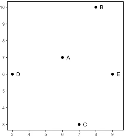
of MDS solution is shown in Figure 1.1 which is a two-dimensional configuration of five objects: A, B, C, D andE. Suppose we would like to know: (1) how dissimilar AandD

(31)

object coordinates in Eq 1.8. That is, δAD =

(zA1−zD1)2+ (zA2−zD2)2

1/2

=

(6−3)2+ (7−6)21/2 = 3.16. Similarly, δAC =

(zA1−zC1)2+ (zA2−zC2)2

1/2

=

(6−7)2+ (7−3)21/2= 4.1. Thus, objectAis more similar toDthan to objectC. The MDS problem is the reverse of this calculation: it is to find the coordinates of the points given the proximities.

Figure 1.1: MDS Model: A two-dimensional configuration of dissimilarity data with five objects (i.e.,A, B, C, DandE).

1.4.2 Multidimensional Unfolding

(32)

1.4. DISTANCE MODELS 9 between a subject (usually a person) and an object (usually a product). For example, preference of students about study courses, preference of customers about set of product designs, preference of instructors about teaching methodology, etc. In this case, subjects are asked to rank their preference for a set of objects or stimuli.

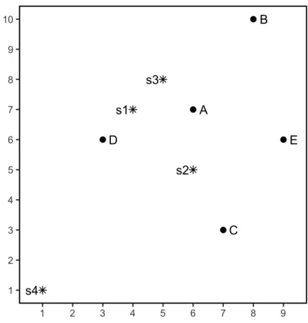
Figure 1.2: MDU Model: A two-dimensional configuration of preference data with four subjects (i.e.,s1, s2, s3ands4) and five objects (i.e.,A, B, C, DandE).

The objective of MDU is to find distances in Euclidean space between subjects and objects that approximate a set of proximities as well as possible (Heiser, 1981, 1987; De Leeuw, 2005). An example of MDU is shown in Figure 1.2 which is the same configuration as Figure 1.1 with respect to the objects and with additional points for the subjects.

(33)

The closer an object or stimulus to the ideal, the more it will be preferred (Davison, 1983, pp. 7). Suppose we would like to know which object (AorC) in Figure 1.2 most preferred by the fourth subject. This question can be answered by working out Eq 1.8. That is, δS4,A =

(zS4,1−zA1)2+ (zS4,2−zA2)2

1/2

= (1−6)2+ (1−7)21/2 = 7.81. Similarly, δS4,C =

(zS4,1−zC1)2+ (zS4,2−zC2)2

1/2

=

(1−7)2_{+ (1}₋₃₎21/2

=

6.3. Thus, this subject prefers object C since the object is closer to its ideal position. Analogous to MDS, the unfolding problem is the reverse of this calculation: it is to find the coordinates of the object points and ideal points given the proximities between object and subjects.

1.4.3 IPDA Model

Takane, Bozdogan, and Shibayama (1987) proposed Ideal Point Discriminant Analysis (IPDA). The IPDA model is a multidimensional unfolding technique used for classification of subjects. The input data of IPDA model are not preference data but classification data, i.e., a given subject would choose one and only one object from a set of categories. The probability for thek−th category in the IPDA model is defined as (Takane, Bozdogan, & Shibayama, 1987),

πk(xi) =

mkexp(−δ2ik) P

cmcexp(−δ2ic)

, (1.9)

wheremk is a bias parameter for categorykwhich can be interpreted as a prior probability

of the class, andδ2

ikis the squared Euclidean distance in anM−dimensional space between

an ideal point for subject i with coordinates ηim and a class point for category k with

coordinatesγkm (Takane et al., 1987), i.e.,

δik2 = M X

m=1

(34)

1.4. DISTANCE MODELS 11 The ideal points are assumed to be a linear combination of the explanatory variables:

ηi=β0+xiβ,

where β is a(p×M) matrix with regression weights and,β0 anM dimensional vector

with intercepts. The parameters of this model are the regression weights and the class points. The class points, denoted asγ, is a matrix of dimension (C×M).

The MBCL model, i.e., Eq. (1.4) and (1.5), is equivalent to the IPDA model in maximum dimensionality, i.e.,M = (C−1)whereC is number of categories or objects.

1.4.4 IPC Model

De Rooij (2009a) proposed the Ideal Point Classification (IPC) model. The IPC model is a probabilistic multidimensional unfolding model and closely related to the IPDA model. As noted by Takane et al (1998), the interpretation of IPDA model is hampered by the bias parameters. De Rooij (2009a) showed that the bias parameters can be ignored without loss of information, except when (1) the response variable has many categories and a low-dimensional distance model is used; and (2) the response variable has a category that dominates the other categories. The probability for thek−th category in the IPC model is defined as (De Rooij, 2009a),

πk(xi) =

exp(−0.5∗δ2

ik) P

cexp(−0.5∗δ2ic)

. (1.11)

By looking at Eq. (1.9) and Eq. (1.11), it can be seen that IPC model is equivalent to the IPDA model without the bias parameters. The log-odds representation of the IPC model is,

logit[πk(xi)] = 0.5∗δib2 −0.5∗δ

2

(35)

where δ2

ib is the squared Euclidean distance between the b-th baseline category and the

ideal point for subject i.

IPC Model for Binary Data

De Rooij (2009a) showed that logistic regression for a binary response variable, i.e., Eq. (1.2) and (1.3), can be expressed as an unidimensional IPC model. That is, a distance model in a joint space with points representing the two categories of the response variable and points representing the subjects.

TheunidimensionalIPC model of the binary response variable which is a simplification of Eq. (1.11) becomes,

π(xi) =

exp(−0.5∗δ2

i1) exp(−0.5∗δ2

i0) + exp(−0.5∗δi21)

. (1.13)

The class points of theunidimensionalIPC model are given byγ=

γ01, γ11

T ,where

γ01is the class point of the baseline category (i.e., Y = 0), andγ11is the class point of

the “success” category (i.e.,Y = 1). The log-odds representation of the unidimensional

IPC model is,

logit[π(xi)] = 0.5∗δi20−0.5∗δ 2

i1

= 0.5∗(ηi1−γ01)2−0.5∗(ηi1−γ11)2

= (γ11−γ01)∗ηi1+ 0.5∗(γ012 −γ 2 11).

(1.14)

With a restriction on class points for model identification (e.g., γ =

0, 1

T

), the

unidimensional IPC model can be simplified to,

(36)

1.4. DISTANCE MODELS 13 Thus, the unidimensional IPC model is equivalent to the binary logistic regression pre-sented in Eq. (1.2) and (1.3) and has the same regression coefficients (i.e., β) and an intercept with an offset of half (i.e.,βIPC0 =β0LR+ 0.5).

IPC Model for Multicategory Data

As shown in Eq. (1.5), MBCL model is a natural extension of a simple LR model for nominal response variable. De Rooij (2009a) also showed that IPC model in a maximum dimensional space (i.e.,M =C−1) is equivalent to the MBCL model.

The log-odds representation of IPC model for a multicategory response variable is given in Eq. 1.12. By setting constraints on the class points, the IPC model can be identified uniquely. Suppose we have a multicategory response variableGwith four categories such as c = 0,1,2,3. For model identification, the class points in a maximum dimensional space (M = 3) can be represented as follows,

γ=



       

0 0 0

1 0 0

0 1 0

0 0 1



       

. (1.16)

That is, the first category (probably the baseline) is positioned on the origin (i.e.,γ1m=

0 0 0

), the second category is on the x−axis (i.e., γ2m =

1 0 0

), the third category is on the y−axis (i.e., γ3m=

0 1 0

), and the fourth category is on the

z−axis (i.e., γ4m =

0 0 1

(37)

against the baseline (i.e.,c= 0). That is,

logit[π1(xi)] = 0.5∗δi20−0.5∗δ 2

i1

= 0.5∗

3

X

m=1

(ηim−γ0m)2−0.5∗

3

X

m=1

(ηim−γ1m)2

= 3

X

m=1

(γ1m−γ0m)∗ηim+ 0.5∗

3

X

m=1

(γ02m−γ12m)

=ηi1−0.5

= (β01−0.5) +β1Txi.

(1.17)

Similarly, the log-odds for the third category: logit[π2(xi)] =ηi2−0.5 = (β02−0.5)+β2Txi,

and the log-odds for the fourth category: logit[π3(xi)] =ηi3−0.5 = (β03−0.5) +β3Txi.

Thus, β_pIPC = β_pMBCL for regression coefficients with dimension (p×M), and β₀IPC = βMBCL0 −0.5 for intercepts with dimension (1×M).

1.5 Multivariate Binary Data

In the previous sections, we considered only a single binary or multicategory response variable. However, it is not uncommon to see multiple binary/multicategory response variables in a given study. In medical science, for example, researchers are often interested not only on the efficacy of a newly developed drug, but also on the side effect of the drug. The explanatory variables in such a drug study setting could be the type of treatment (i.e., placebo, current drug, and newly developed drug), age, gender, etc. In this hypothetical study, there are two binary responses: efficacy (i.e., whether the subject is cured or not), and side effect (i.e., whether the drug has a side effect or not).

(38)

1.5. MULTIVARIATE BINARY DATA 15 example, researchers investigated impact of exposure to smoking and pneumoconiosis on two respiratory diseases, breathlessness (1 =yes;0 =no) and wheeze (1 =yes;0 =no), of coalminers in Britain (Ashford, Morgan, Rae, & Sowden, 1970; McCullagh & Nelder, 1989; Palmgren, 1989).

Another example of multivariate binary data is the Netherlands Study of Depression and Anxiety (NESDA). In NESDA, data were collected to investigate the interplay between personality traits and co-morbidity of depressive and anxiety disorders (Penninx et al., 2008; Spinhoven, De Rooij, Heiser, Penninx, & Smit, 2009). Co-morbidity is a presence of two or more mental disorders. In the area of mental disorders clinical psychologists and epidemiologists are interested in co-morbidity and how co-morbidity is related to risk factors such as personality traits and background variables (Krueger, 1999; Beesdo-Baum et al., 2009; Spinhoven, Penelo, De Rooij, Penninx, & Ormel, 2013). The NESDA data will be a leading example throughout this dissertation. We thank the NESDA consortium for providing the data.

Another study in which multivariate binary data arises is the Indonesian Children’s Study (ICS: Sommer, Katz, & Tarwotjo, 1984; Liang, Zeger, & Qaqish, 1992) where over three-thousand children were medically examined to investigate whether they had respi-ratory infection, diarrhoeal infection, and xerophthalmia. The aim of the ICS study was to investigate whether vitamin A deficiency places children at increased risk of respiratory and diarrhoeal infections.

Supposey_i= (yi1, yi2, . . . , yij, . . . , yiJ)T denotes the multivariate responses observed

on the i−th subject, which is a (J ×1)-dimensional vector of all responses. The yij

(39)

The other columns in Table 1.1 have measurements for explanatory variables X1, X2, . . . ,

Xp.

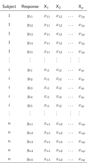
Table 1.1: The structure of multivariate data in long format.

Explanatory variables

Subject Response X1 X2 Xp

1 y11 x11 x12 . . . x1p

1 y12 x11 x12 . . . x1p

1 y13 x11 x12 . . . x1p

1 y14 x11 x12 . . . x1p

1 y15 x11 x12 . . . x1p

..

. ... ... ... ... ...

i yi1 xi1 xi2 . . . xip

..

. ... ... ... ... ...

n yn1 xn1 xn2 . . . xnp

(40)

1.5. MULTIVARIATE BINARY DATA 17

1.5.1 Bivariate Binary Data

Two cross classified binary variables observed on the i-th subject is displayed in Table 1.2. The rows represent measurements of the first binary response variable (y_i₁), and the columns represent measurements of the second response variable (yi2). In this Table,

both marginal probabilities (shown in the margins, i.e.,πi1.,πi0., πi.1, andπi.0) and the

joint probabilities (shown in the four cells, i.e.,πi,11,πi,10,πi,01, andπi,00) are presented.

The sum of probabilities either for the margins by row/column or for the individual cells always equals one.

Empirical researchers working with bivariate binary data are often interested in one of the following thee parameters (Ashford et al., 1970; MacLean, Sofuoglu, & Rosenheck, 2018; Bhuyan, Islam, & Rahman, 2018): (1) the marginal probabilities; (2) the association between the two binary responses; or (3) the joint (or multinomial) probabilities.

Table 1.2: Cross-classification of measurements of a bivariate binary data observed on thei-th subject.

y_i₂

1 0

yi1 1 πi,11 πi,10 πi1.

0 πi,01 πi,00 πi0. πi.1 πi.0 1.00

Joint Probabilities

The joint probability is an important quantity of bivariate binary data. In the Coalminers study, for example, let y_i₁and y_i₂denotes the measurements of breathlessness and wheeze of the coalminers, respectively. Then, the joint probabilityπi,10represents the probability

of getting breathlessness, but no wheeze. Similarly, the joint probabilityπi,01 represents

(41)

the diseases (πi,00).

Bivariate binary data are special case of a multicategory response variable with four categories. Therefore, we can use a single index to represent the joint probabilities, i.e.,

πik(xi) =Pr(Gi=k|xi). For the joint probabilities in Table 1.2, this means: πi1=πi,00,

πi2=πi,10,πi3=πi,01, andπi4=πi,11. Because of this relationship, logistic regression

models for a multicategory response data such as the MBCL model (Eq. 1.4 and 1.5) and the IPC model (Eq. 1.11 and 1.12), can be used to analyze the joint probabilities of bivariate binary data.

Marginal Probabilities

The marginal probability of a bivariate binary data models a single response variable without controlling for measurements of the second response variable. Two separate simple logistic regression models (Eq. 1.2 and 1.3) can be used for this purpose, one for each response variable. In the Coalminers study, the marginal model can be used to answer a question about probability of breathlessness (wheeze) of coalminers due to exposure.

Association

The third quantity of interest is the association between the binary response variables. The association gives us information about the relationship of the two binary response variables. That is, it tells us whether the probability of occurrence of the second response variable increase/decrease when the probability of occurrence of the first response variable increases, and vice versa.

(42)

1.6. MODELS FOR MULTIVARIATE BINARY DATA 19 That is,

log (τi) =β0+βTxi, (1.18)

whereτi denotes the OR and is defined asτi= (πi4×πi1)/(πi2×πi3).

1.6 Models for Multivariate Binary Data

The most common statistical modeling approach for analyzing multivariate binary re-sponses in the presence of explanatory variables, are (1) marginal models (Agresti, 2002, Chap 11), and (2) latent variable models (Agresti, 2002, Chap 12). Marginal models are sometimes referred to as population-averaged models. Latent variable models are sometimes referred to asrandom-effects orsubject-specific models.

1.6.1 Marginal Models

(43)

1.6.2 Latent Variable Modeling

Latent variable models are a general class of models that are used for analyzing multi-variate data (Bartholomew & Knott, 1999; Skrondal & Rabe-Hesketh, 2004). In Latent Variable (LV) models the multivariate response variables are treated as dependent vari-ables, and one or more unobserved varivari-ables, referred to as latent varivari-ables, are treated as independent variables. The response variables are sometimes called indicators because they are used as an indirect measure of the latent variables.

The main application of LV models are: (1) for reducing the dimensionality of the multivariate data (to explain the variation of observed variables in few dimensions), (2) as measurement model (for representing a concept or construct that cannot be directly mea-sured, e.g., depression, quality of life, political attitude, mathematical ability, intelligence, etc), and (3) for assigning scores on the latent scale which correspond to subjects’ profile (Bartholomew, Steele, Moustaki, & Galbraith, 2002; Bollen, 2002; Rizopoulos, 2006). Tomarken and Waller (2005) provided a detailed literature review on Structural Equation Modeling (SEM) focusing on its strengths, limitations, and misconceptions.

Confirmatory Factor Analysis of Multivariate Data

Let y_i = (y_i₁,y_i₂, . . . ,y_ij) be a j-dimensional vector of interval indicator variables ob-served on the i-th subject. The Confirmatory Factor Analysis (CFA) is based on the as-sumption thatyi can be attributed toqcommon factors, denoted byθi= (θi1, . . . , θiq),

(44)

1.6. MODELS FOR MULTIVARIATE BINARY DATA 21

θ1 θ2

y1 y2 y3 y4 y5 y6

1 2 3 4 5 6

λ11 λ21

λ31

λ42 λ52

λ62

ψ12

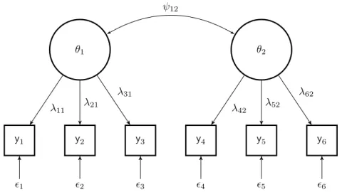
Figure 1.3: A path diagram of a CFA with six indicator variables represented by a square, and two latent variables represented by a circle.

(Thurstone, 1947; J¨oreskog & S¨orbom, 1981). The CFA is defined as,

y_i₁ =λ11θi1+. . .+λ1qθiq+i1

yi2 =λ21θi1+. . .+λ2qθiq+i2

.. .

y_ij =λp1θi1+. . .+λjqθiq+ij

or, in matrix form

y_i=Λθi+i, (1.19)

where Λ is the matrix of factor loadings. Let Ψ be the covariance matrix of common factors, and let Φ be the covariance matrix of the unique factors. In Figure 2.1 an example of a path diagram is displayed which corresponds to a measurement model with six indicators (j= 6) and two underlying latent variables (q= 2).

(45)

distribu-tions, i.e., θ ∼ Nq(0,Ψ) and ∼Nj(0,Φ), where Φ is a diagonal matrix. Given the

model, the expected covariance matrix of the indicator variables becomes

Σ=ΛΨΛT+Φ. (1.20)

CFA for Multivariate Dichotomous Data

CFA was originally developed for modeling interval indicator variables. The covariance or correlation matrix of the observed variables was used as a primary object of analysis. The same method was later proposed for handling categorical (or dichotomous) indicator variables (Christoffersson, 1975; B. Muthen, 1978).

Let yi = (yi1, yi2, . . . , yij, . . . , yiJ) be a J−dimensional vector of dichotomous

in-dicator variables observed on the i-th subject. CFA of dichotomous variables assumes an underlying latent variable for each indicator variable, which is denoted by y∗_i = (y_i∗₁, y_i∗₂, . . . , y∗_ij, . . . , y∗_iJ). Thus, the variableyij equals one if its underlying latent

vari-able y∗_ij is above a certain threshold value τj, otherwise it equals zero. Therefore, the

measurement model fory_i is given by

y∗i =Λθi+i, yij =    

  

1, if y_ij∗ ≥τj,

0, if y_ij∗ < τj.

(1.21)

The formula for the covariance matrix remains the same, i.e., V(y∗) = Σ, but the elements in Φmatrix are not free parameters anymore, rather

Φ=I−diag(ΛΨΛT), (1.22)

yielding diag(Σ) =I. Therefore, the model has three sets of free parameters: τ,Λ, and

(46)

1.6. MODELS FOR MULTIVARIATE BINARY DATA 23

Multivariate Regression with Latent Variables: The MIMIC Model

The measurement model is often not an ultimate step since researchers are interested in group differences and/or measurement invariance on the latent variables (Stapleton, 1978; Kenneth, 1989; T. Brown, 2006). This can be done by including external variables into CFA, and the new model becomes the Multiple Indicators MultIple Causes (MIMIC) model (J¨oreskog & Goldberger, 1975; B. Muthen, 1983, 1984).

Letxi= (xi1, xi2, . . . , xip)be the external variables observed on thei-th subject.

Fig-ure 2.2 shows the path diagram for a MIMIC model with two external variables connected to the two common latent variables. The MIMIC model extends the CFA model presented in (1.19) with relationships between the latent variables and the external variables, i.e.,

y_i = Λθi+i

θi = ΓTxi+ζi, (1.23)

whereΓgives the regression coefficients, andζthe structural disturbances. It is assumed that the disturbances and the measurement errors are uncorrelated to each other and to

x, but not necessarily among themselves. The covariance matrix of the latent variables now becomes

Ψ=ΓTΣxΓ+Σζ,

where Σx is a covariance matrix for the external variables, and Σζ for the disturbances.

(47)

θ1 θ2

y1 y2 y3 y4 y5 y6

x1 x2

1 2 3 4 5 6

ζ1 ζ2

λ11 λ21

λ31

λ42 λ52

λ62

γ11

γ12

γ21

γ22

ψ12

Figure 1.4: A path diagram for a MIMIC model with two external variables that are represented by a square.

1.7 Outline of the Thesis

Latent variable models are often used for analyzing multivariate binary data with and without the presence of explanatory variables. In Chapter 2 we investigate the performance of such models using a simulation study. We show the impact of the number of indicator variables, sample size, and type of indicator variables, on the performance of latent variable models.

(48)

1.7. OUTLINE OF THE THESIS 25 to fully recover parameters of interest for bivariate binary data.

However, it is not straight forward to extend the BIPC model for the analysis of multivariate binary data. This is due to the fact that both the pairwise and higher-order association structure parameters must be specified in the likelihood function, and thus the computation becomes cumbersome. This issue will be addressed in Chapter 4 by developing a Multivariate Logistic Distance (MLD) model which is a new model for analyzing multivariate binary data. The MLD model unifies two domains of statistical methods, i.e., Multidimensional Scaling (MDS: Kruskal & Wish, 1978; Borg & Groenen, 2005) and Generalized Linear Model (GLM: McCullagh & Nelder, 1989; Agresti, 2002). As a form of regularization, the MLD model allows for dimension reduction and therefore less parameters are estimated compared to existing marginal models for multivariate binary data. Moreover, the model enhances interpretation by using a biplot (Gabriel, 1971; Gower & Hand, 1996; Gower, Lubbe, & Le Roux, 2011) based on a distance interpretation.

(49)

(50)

Chapter 2 Effects of a Small Number of Dichotomous Indicators in

Latent Variable Modeling: A Simulation Study

Abstract

Structural equation models were originally proposed for the analysis of continuous or inter-val indicator variables. Recently, factor analysis and structural equation models have been applied for data with dichotomous indicators and with only a few indicators per latent variable, i.e. 2 or 3. We investigated the performance of Confirmatory Factor Analy-sis (CFA) and the Multiple Indicators MultIple Causes (MIMIC) model for dichotomous indicators in comparison with interval indicators in a Monte Carlo simulation study.

The performance of both CFA and the MIMIC model was studied in terms of the quality of recovering the true factor scores and the incidence of improper solutions, more specifically non-convergence andHeywood cases. Furthermore, in the case of the MIMIC model, the focus was on the type-I error rate and power.

We showed that both CFA and the MIMIC model performed poorly with a small number of dichotomous indicators, i.e., (1) improper solutions occurred much more fre-quently; (2) the true factor scores are poorly recovered; (3) the type-I error rates are too conservative mostly and inflated sometimes; and (4) the observed power was weak.

(51)

2.1 Introduction

Latent variable models are a general class of models that are used for analyzing multi-variate data (Bartholomew & Knott, 1999; Skrondal & Rabe-Hesketh, 2004). In Latent Variable (LV) models the multivariate observed variables (manifest variables) are treated as dependent variable, and one or more unobserved variables (latent variables) are treated as independent variables. The observed variables are also known as indicators because they are used as an indirect measure of the latent variables.

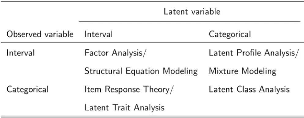
The Latent variables can be interval or categorical. As displayed in Table 2.1, there are four classes of LV models based on the cross-classification of whether the observed variable and/or latent variable is interval and/or categorical (Bartholomew & Knott, 1999). Our main focus in this paper will be on Confirmatory Factor Analysis (CFA), which is a special case of Structural Equation Modeling (SEM: Thurstone, 1947; J¨oreskog & S¨orbom, 1981; Christoffersson, 1975; B. Muthen, 1978; Bock & Lieberman, 1970; Mislevy, 1986). Tomarken and Waller (2005) provided a detailed literature review on Structural Equation Modeling (SEM) focusing on its strengths, limitations, and misconceptions.

Table 2.1: Classes of Latent Variable Models.

Latent variable Observed variable Interval Categorical

Interval Factor Analysis/ Latent Profile Analysis/ Structural Equation Modeling Mixture Modeling Categorical Item Response Theory/ Latent Class Analysis

Latent Trait Analysis

(52)

2.1. INTRODUCTION 29 equation models (Boomsma, 1983, 1985; J. C. Anderson & Gerbing, 1984; Acito & An-derson, 1986). Recently, in clinical psychological research structural equation models have been proposed for the analysis of comorbidity of depressive and anxiety disorders (Krueger, 1999; Beesdo-Baum et al., 2009). A typical characteristic of these models is that the indicators are dichotomous, i.e the indicators indicate whether someone has or does not have a particular disorder, and that there are only a few indicators per latent variable, i.e. 2 or 3. We believe the application of structural equation models in such a scenario (i.e., dichotomous indicators with a few number of variables per factor) is not adequate enough to obtain a valid result about the research question that we would like to answer. This is because with two indicator variables, there are only four patterns (i.e., (0, 0), (0, 1), (1, 0), and (1, 1)) with four corresponding observed proportions. Similarly, for three indicators, there will be eight patterns. Therefore, there is only limited information and it is hard to satisfy the normality assumption of the underlying latent variables in the structural equation model. However, we did not find large scale simulation studies that address our concerns. The aim of the current paper is to fill this gap. Therefore, we conducted a simulation study to investigate the performance of SEM for the analysis of a small number of dichotomous indicator variables per factor.

(53)

indicators, strength of factor structure, correlation between factor scores, and sample size. The outline of this paper is as follows. In Section 2.2 we discuss issues with factor analysis and results found in the literature. The design and analysis of the simulation study is presented in Section 2.3. In Section 2.4, the results of the simulation studies are discussed. We conclude with a discussion of the results and some remarks for future research in Section 2.5.

2.2 Issues with Factor Models for Multivariate Data

2.2.1 Indeterminacy of Factor Scores

The indeterminacy of factor scores refers to a situation where the same indicator variables may produce different factor scores with the same model fit, and thus no unique solution does exist for the factor scores (Acito & Anderson, 1986; Guttman, 1955; Heermann, 1964, 1966; Schonemann, 1971; Schonemann & Wong, 1972; Green, 1976; Elffers, Bethlehem, & Gill, 1978). Some argue that the reason for the indeterminacy of factor scores is due to the presence of too many parameters compared to the number of equations in the model (Grice, 2001).

2.2.2 Improper Solutions

(54)

2.2. ISSUES WITH FACTOR MODELS FOR MULTIVARIATE DATA 31

2.2.3 Previous Studies

Indeterminacy of factor scores in CFA has been studied by Acito and Anderson (1986). The impact of the number of indicators, factoring method, factor structure (i.e., the magnitude of factor loadings), number of factors, and sample size on indeterminacy of factor scores was investigated. Acito and Anderson found that both the factor structure and the factoring method have large effects on the indeterminacy of factor scores. A limitation of their study was that only interval indicators were considered. In the current study we also consider dichotomous indicators.

Improper solutions, i.e., nonconvergence andHeywood cases, in CFA has been studied using a Monte Carlo simulation by Anderson and Gerbing (1984) and by Boomsma (1985). Anderson and Gerbing studied the impact of sampling error and model characteristics on the incidence of improper solutions. Improper solutions occurred more frequently for smaller sample sizes and for models with fewer indicators for each factor (J. C. Anderson & Gerbing, 1984). Boomsma studied the impact of the number of indicators, correlation between factors, and factor structure. All of the design variables had a large effect on the incidence of improper solutions (Boomsma, 1985). Like the study by Acito and Anderson (1986), however, both studies considered only interval indicators. In this paper, we extend their study on improper solutions by including both interval and dichotomous indicator variables.

(55)

Velicer, and Harlow (1995), Kenny and McCaoch (2003) and Marsh, Balla, and McDonald (1988), although the main focus of these studies was on measures of fit for factor models. In general, all these studies investigated the impact of variables of interest on statistical properties of CFA when the indicator variables are interval. Categorical (or dichotomous) indicator variables were not considered. Furthermore, emphasis was given for factor models and the MIMIC model was not studied in a similar fashion. Our present simulation study fills these gaps since both issues are addressed.

2.3 Monte Carlo Simulation Study

We followed the six-step approach of Monte Carlo simulation design in structural equation modelling (Paxton, Curran, Bollen, Kirby, & Fen, 2001; Skrondal, 2000; Boomsma, 2013).

2.3.1 The Research Problem

Our main objective is to investigate the performance of SEM models, specifically Con-firmatory Factor Analysis (CFA) and the MIMIC model, with only a few dichotomous indicators assumed per factor. We investigate the quality of recovering the true factor scores and the incidence of improper solutions (nonconvergence andHeywood cases). We study the impact of five design variables on the outcome variables. To have a benchmark to compare the performance of latent variable models for analyzing dichotomous indicator variables, we also consider interval indicator variables. We used Mplus statistical soft-ware package (L. Muthen & Muthen, 1998-2012) with the default estimation procedures to analyze our simulated datasets, because that is how most applied researchers analyze their data.

(56)

2.3. MONTE CARLO SIMULATION STUDY 33 we study the performance of CFA and in the second experiment the performance of the MIMIC model.

2.3.2 Experimental Plan

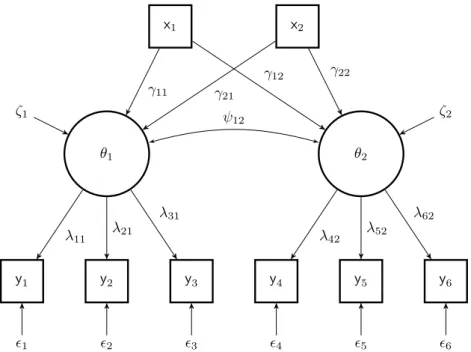
The simulated data were generated from a 2-factor model whose path diagram is shown in Figure 2.1 for the CFA and in Figure 2.2 for the MIMIC model. In the path diagrams we have six observed variablesyj (j= 1,2, . . . ,6), two latent variablesθq (q= 1,2), and

unique factors indicated byj. The model parameters in CFA are the factor loadingsλjq

and the covariance between the latent variablesψ12.

In the case of the MIMIC model (Figure 2.2) explanatory variables (xk, k = 1,2) are

added to the path diagrams. In addition to parameters of the factor model, the MIMIC model also has regression weights (γkq).

(57)

θ1 θ2

y1 y2 y3 y4 y5 y6

1 2 3 4 5 6

λ11 λ21

λ31

λ42 λ52

λ62

ψ12

Figure 2.1: A path diagram of a factor model with six indicator variables represented by a square, and two latent variables represented by a circle.

θ1 θ2

y1 y2 y3 y4 y5 y6

x1 x2

1 2 3 4 5 6

ζ1 ζ2

λ11 λ21

λ31

λ42 λ52

λ62

γ11

γ12

γ21

γ22

ψ12

(58)

2.3. MONTE CARLO SIMULATION STUDY 35

Table 2.2: The design variables with their corresponding values (or ranges) that are considered in the Monte Carlo simulation study. BLR stands for Binary indicator variables with Low success Rates; and BMR for Binary indicator variables with Moderate success Rates.

Variable Parameter Level Value/Range

Type of Indicators − BLR 5%−15%

BMR 40%−50%

Interval −

Number of Indicators J Few 6

Medium 10

Large 16

Factor structure λjq Weak (0.316,0.447)

Moderate (0.316,0.632)

Strong (0.632,0.775)

Correlation between Factors ψ12 Independence 0.0

Moderate 0.4

Strong 0.8

Sample size N Very Small 50

Small 100

Big 300

Very Big 3,000

For the number of indicators, Anderson and Gerbing (1984) suggested at least 3 indicators per factor in CFA. Kenny and McCoach (2003) varied the number of indicators from four to twenty-five to assess the impact on measures of fit. The number of indicators in our simulation study was varied from 3 to 8 per factor, which is equivalent toJ = 6to

J = 16indicators in total. For the factor structure, we used the ranges proposed by Acito and Anderson (1986). Both factor structure and variances for the measurement errors can be derived from the factor loadings, i.e., ψ11 = P

J j=1λ

2

j1 and ψ22 = P

J j=1λ

2

(59)

and φj = 1−λ2j, respectively. In our simulation study, following Acito and Anderson

(1986), we set factor loading values to: (0.316,0.447)for weak structure,(0.316,0.632)

for moderate structure, and(0.632,0.775) for strong structure.

For the sample size, Boomsma (1985) recommended a sample size of at leastN = 50

and Anderson and Gerbing (1984) suggested a sample size of at leastN = 150. Boomsma and Hoogland (2001) showed that a sample size below N = 200 is vulnerable for the occurrence of improper solutions. In our Monte Carlo simulation the sample size was varied fromN = 50toN = 3,000. Three possible situations for the correlation between the latent variables were considered: ψ12 = 0.0 (independence), ψ12 = 0.4 (moderate

association), andψ12= 0.8(strong association).

2.3.3 Simulation

The simulated data is generated following the MIMIC model. In the simulated MIMIC model eight explanatory variables were considered. The true values that are used in the simulation study are based on the fitted MIMIC model on the NESDA data (Penninx et al., 2008). The first explanatory variable was generated from a Binomial distribution and the others from a Standard Normal distribution, i.e., x1 ∼Bin(0.67)andxk ∼N(0,1)

fork= 2, . . . ,8. The regression coefficients used in the simulation are the following, for

x1: γ11 = γ12 = 0.00; x2: γ21 = −0.10, γ22 = −0.20; x3: γ31 = γ32 = 0.00; x4:

γ41 = 1.00, γ42 = 0.95; x5: γ51 =−0.30, γ52 = −0.25; x6: γ61 = γ62 = 0.00; x7:

γ71= 0.00,γ72= 0.10; andx8: γ81=γ82= 0.00.

Factor structures were then generated from a bivariate normal distributionθ∼N2(µ,Ψ),

where

µ=



 

µ1

µ2



 =



 

γT

1x+ζ1 γT

2x+ζ2



(60)

2.3. MONTE CARLO SIMULATION STUDY 37 and

Ψ=



 

ψ11 ψ12

ψ21 ψ22



 =



 

γ₁TΣxγ1+Var(ζ1) ψ12

ψ12 γ2TΣxγ2+Var(ζ2)



 ,

whereγ1 is a vector of regression coefficients for the first factor, and similarlyγ2for the second factor.

2.3.4 Estimation

For each simulated data set a 2-factor model was fitted with and without explanatory vari-ables, which corresponds to the CFA and the MIMIC model, respectively. The analysis was done using theMplus statistical software version 7 (L. Muthen & Muthen, 1998-2012). A Maximum Likelihood Robust (MLR) estimator was employed for interval indicators whereas a Weighted Least Square estimator with Mean and Variance adjusted (WLSMV) was used for dichotomous indicator variables. The WLSMV is the default estimator in

Mplus. We used the package called MplusAutomation (Hallquist, 2012) to help us call and runMplusfrom theRenvironment.

The analysis procedure in our Monte Carlo simulation can be summarized as follows, 1. Fit a 2-factor CFA (or MIMIC model) on the simulated data.

2. Check if the fitted model is estimated without any problem due to improper so-lutions. Otherwise, identify the problem and record as nonconvergence and/or

Heywood.

3. Estimate the factor scores, i.e.,θˆ= (ˆθ1,θˆ2).

4. If the fitted model is estimated correctly, calculate the correlation between true and estimated factor scores, i.e., ρq =Corr(θq,θˆq) where q= 1,2. In the case of the

(61)

(a) the type-I error rate the regression coefficients. (b) the power of the regression coefficients. 5. Repeat Step 1 to 4 for each simulated data set.

2.3.5 Replication

In our Monte Carlo simulation we use a full factorial 3×3×3×3×4 design, with in total 324 In each cell we useR= 100replications.

2.3.6 Analysis of Output

For the first experiment, the variables of interest are the incidence of improper solutions and the quality of recovering the true factor scores in CFA .

The incidence of improper solutions was analyzed using a logistic regression model (Agresti, 2002). When a low rate of improper solutions is found in the data, Firth logistic regression (FLR: Firth, 1993) was used because it yields finite parameter estimates in the presence of complete or quasi-complete separation (Heinze & Schemper, 2002). SAS

version 9.4 was used to fit the logistic regression models (SAS Institute Inc., 2013). The Odds Ratio (OR) was used as an effect size measure for evaluating the practical signifi-cance of the design variables and their interactions. We used the guidelines suggested by Ferguson (2009), i.e., an odds ratio of about 2 (or 0.50) indicates a small effect, about 3 (or 0.33) a medium effect, and about 4 (or 0.25) a large effect. For interpretation of sim-ulation results, we focus on large effects for type of indicators and number of indicators, and their interactions with the other design variables.

Analysis of Variance (ANOVA) was used for analyzing the correlation data, i.e.,ρ1and

ρ2, to assess the impact of design variables on the quality of recovering the true factor

scores. Because ρ1 andρ2 are very similar we focus on ρ1. A Fisher’s transformation is

(62)

2.4. RESULTS 39 We usedSPSS version 21 to fit the ANOVA model (IBM SPSS, 2012). The partial eta squared, denoted by η2, will be used as a measure of effect size for the ANOVA model. According to Cohen (1988), a value of η2= 0.01 indicates a small effect,η2 = 0.059 a medium effect, andη2= 0.138a large effect. For interpretation of simulation results, we focus on large effects for type of indicators and number of indicators, and their interactions with the other design variables.

In the second experiment we are further interested in the type-I error rate and the power for the regression weights of the MIMIC model. These measures were obtained by first calculating the proportion of cases in which an effect becomes statistically significant. For the effects equal to zero, the calculated proportion represents the type-I error rate; otherwise, the proportion corresponds to the power of the test. In the case of type-I error rate, a95%confidence interval of the proportion using the Wilson interval was calculated (L. D. Brown, Cai, & DasGupta, 2001).

2.4 Results

2.4.1 Experiment-I: Confirmatory Factor Analysis

Nonconvergence in CFA

About18.9%of the analyses in our simulation study did not converge. We applied logistic regression on the nonconvergence outcome variable (1: not converged; 0: converged) to investigate the impact of the design variables. The observed proportions of nonconver-gence cross classified by design variables are presented in Table 2.3. A two-way interaction logistic model was fitted to the nonconvergence data.

(63)

(64)

2.4. RESULTS 41 of indicators has a large effect on the incidence of nonconvergence in CFA. Moreover, we found a large effect of 2-way interaction between the type of indicators and the following variables: number of indicators, factor structure, and sample size. There is also a large effect of number of indicators on the incidence of nonconvergence in CFA, and its 2-way interaction with the sample size. Figure 2.3 displays the corresponding interaction plots for the large effects. The first three panels (from left to right) show interaction plot between the type of indicators and the other design variables (i.e., the number of indicators, the factor structure, and the sample size). The last panel is for the interaction plot between the number of indicators and the sample size.

Regardless of the other design variables (i.e., number of indicators, factor structure, and sample size), we found a large effect of type of indicators on the prevalence of non-convergence in CFA. The worst result was obtained for the binary indicators, specifically for the BLR data. For interval indicators, there was not much effect of the other design variables on the prevalence of nonconvergence in CFA.

(65)

Figure 2.3: Interaction plot for Nonconvergence rate: The first three panels (from left to right) show interaction plot between the type of indicators and the number of indicators, the factor structure, and the sample size, respectively. The last panel is for the interaction between the number of indicators and the sample size.

Heywood cases in CFA

(66)

2.4. RESULTS 43 in Table 2.4. A 2-way interaction logistic model was fitted on theHeywood data, and the results are presented in the Appendix (Table A.2).

Like for the nonconvergence analysis, our focus will be on the effects of the type of indicators and the number of indicators, and their interaction with the other design variables. The type of indicators has a large effect on the incidence ofHeywood in CFA. Moreover, we found a large effect of 2-way interaction between the type of indicators and all the other design variables, i.e., number of indicators, factor structure, correlation between latent variables, and sample size. There is also a large effect of number of indicators on the incidence of nonconvergence in CFA, and its 2-way interaction with both the factor structure and sample size. Figure 2.4 displays the interaction plots for the large effects. The first four panels (from left to right) show interaction plot between the type of indicators with the number of indicators, the factor structure, the correlation between underlying latents, and the sample sizes. The last two panels are for the interaction plot between the number of indicators with the factor structure and sample size.

In the first three panels, it can be seen that there is no large difference in prevalence ofHeywood cases among the type of indicators used in CFA. The fourth panel shows the interaction with the sample size, where the highest number ofHeywood cases was found for the BLR data, except for a large and small data sets.

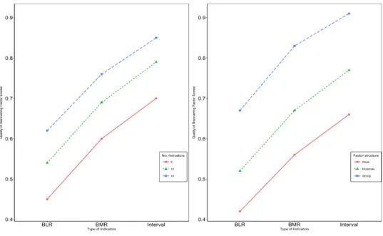
There is a large effect of the number of indicators on the prevalence of Heywood

Distance models for analysis of multivariate binary data

Cover Page

The following handle holds various files of this Leiden University dissertation:

http://hdl.handle.net/1887/67140

Author

: Worku, H.M.

Title:

Distance models for analysis of multivariate binary data

Invitation

to attend the defense

of the thesis

Distance Models

for Analysis of

Multivariate Binary

Data

on Thursday 20 December

2018 at 3.00 pm in

the Academiegebouw of

Leiden University,

Rapenburg 73 in Leiden

Paranymphs:

Maarten Kampert

&

Yinebeb Tessema

Hailemichael Metiku Worku

Distance Models

for Analysis of

M u l t i v a r i a t e

B i n a r y D a t a

Hailemichael Metiku Worku

Distance Models for Analysis of Multivariate Binary Data

Distance Models for Analysis of

Distance Models for Analysis of

Multivariate Binary Data

Contents

Motto

Research Articles

List of Figures

List of Tables

Chapter 1

Introduction

1.1

Categorical Response Data

1.1.1

Binary Response Data

1.1.2

Multicategory Response Data

1.2

Explanatory variables

1.3

Logistic Regression Model

1.3.1

Binary Logistic Regression

1.3.2

Multinomial Logistic Regression

1.3.3

Parameter Estimation in Logistic Regression Models

1.4

Distance Models

1.4.1

Multidimensional Scaling

1.4.2

Multidimensional Unfolding

1.4.3

IPDA Model

1.4.4

IPC Model

1.5

Multivariate Binary Data

1.5.1

Bivariate Binary Data

1.6

Models for Multivariate Binary Data

1.6.1

Marginal Models

1.6.2

Latent Variable Modeling

1.7

Outline of the Thesis

Chapter 2