Search Based Software Engineering: Techniques, Taxonomy, Tutorial

Search Based Software Engineering:

Techniques, Taxonomy, Tutorial

Mark Harman1_{, Phil McMinn}2_{, Jerffeson Teixeira de Souza}3_{, and Shin Yoo}1 1 _{University College London, UK}

2 _{University of Sheffield, UK} 3 _{State University of Cear´a, Brazil}

Abstract. The aim of Search Based Software Engineering (SBSE) research is to move soft-ware engineering problems from human-based search to machine-based search, using a variety of techniques from the metaheuristic search, operations research and evolutionary computa-tion paradigms. The idea is to exploit humans’ creativity and machines’ tenacity and reliabil-ity, rather than requiring humans to perform the more tedious, error prone and thereby costly aspects of the engineering process. SBSE can also provide insights and decision support. This tutorial will present the reader with a step-by-step guide to the application of SBSE tech-niques to Software Engineering. It assumes neither previous knowledge nor experience with Search Based Optimisation. The intention is that the tutorial will cover sufficient material to allow the reader to become productive in successfully applying search based optimisation to a chosen Software Engineering problem of interest.

1

Introduction

Search Based Software Engineering (SBSE) is the name given to a body of work in which Search Based Optimisation is applied to Software Engineering. This approach to Software Engineering has proved to be very successful and generic. It has been a subfield of software engineering for ten years [45], the past five of which have been characterised by an explosion of interest and activity [48]. New application areas within Software Engineering continue to emerge and a body of empirical evidence has now accrued that demonstrates that the search based approach is definitely here to stay.

SBSE seeks to reformulate Software Engineering problems as ‘search problems’ [45, 48]. This is not to be confused with textual or hypertextual searching. Rather, for Search Based Software Engineering, a search problem is one in which optimal or near optimal solutions are sought in a search space of candidate solutions, guided by a fitness function that distinguishes between better and worse solutions. The term SBSE was coined by Harman and Jones [45] in 2001, which was the first paper to advocate Search Based Optimisation as a general approach to Software Engineering, though there were other authors who had previously applied search based optimisation to aspects of Software Engineering.

SBSE has been applied to many fields within the general area of Software Engineering, some of which are already sufficiently mature to warrant their own surveys. For example, there are surveys and overviews, covering SBSE for requirements [111], design [78] and testing [3, 4, 65], as well as general surveys of the whole field of SBSE [21, 36, 48].

This paper does not seek to duplicate these surveys, though some material is repeated from them (with permission), where it is relevant and appropriate. Rather, this paper aims to provide

those unfamiliar with SBSE with a tutorial and practical guide. The aim is that, having read this paper, the reader will be able to begin to develop SBSE solutions to a chosen software engineering problem and will be able to collect and analyse the results of the application of SBSE algorithms.

By the end of the paper, the reader (who is not assumed to have any prior knowledge of SBSE) should be in a position to prepare their own paper on SBSE. The tutorial concludes with a simple step-by-step guide to developing the necessary formulation, implementation, experimentation and results required for the first SBSE paper. The paper is primarily aimed at those who have yet to tackle this first step in publishing results on SBSE. For those who have already published on SBSE, many sections can easily be skipped, though it is hoped that the sections on advanced topics, case studies and the SBSE taxonomy (Sections 7, 8 and 9) will prove useful, even for seasoned Search Based Software Engineers.

The paper contains extensive pointers to the literature and aims to be sufficiently comprehensive, complete and self-contained that the reader should be able to move from a position of no prior knowledge of SBSE to one in which he or she is able to start to get practical results with SBSE and to consider preparing a paper for publication on these results.

The field of SBSE continues to grow rapidly. Many exciting new results and challenges regularly appear. It is hoped that this tutorial will allow many more Software Engineering researchers to explore and experiment with SBSE. We hope to see this work submitted to (and to appear in) the growing number of conferences, workshops and special issue on SBSE as well as the general software engineering literature.

The rest of the paper is organised as follows. Section 2 briefly motivates the paper by setting out some of the characteristics of SBSE that have made it well-suited to a great many Software Engineering problems, making it very widely studied. Sections 3 and 4 describe the most commonly used algorithms in SBSE and the two key ingredients of representation and fitness function. Section 5 presents a simple worked example of the application of SBSE principles in Software Engineering, using Regression Testing as an exemplar. Section 6 presents an overview of techniques commonly used to understand, analyse and interpret results from SBSE. Section 7 describes some of the more advanced techniques that can be used in SBSE to go beyond the simple world of single objectives for which we seek only to find an optimal result. Section 8 presents four case studies of previous work in SBSE, giving examples of the kinds of results obtained. These cover a variety of topics and involve very different software engineering activities, illustrating how generic and widely applicable SBSE is to a wide range of software engineering problem domains. Section 9 presents a taxonomy of problems so far investigated in SBSE research, mapping these onto the optimisation problems that have been formulated to address these problems. Section 10 describes the next steps a researcher should consider in order to conduct (and submit for publication) their first work on SBSE. Finally, Section 11 presents potential limitations of SBSE techniques and ways to overcome them.

2

Why SBSE?

As pointed out by Harman, Mansouri and Zhang [48] Software Engineering questions are often phrased in a language that simply cries out for an optimisation-based solution. For example, a Software Engineer may well find themselves asking questions like these [48]:

1. What is the smallest set of test cases that cover all branches in this program? 2. What is the best way to structure the architecture of this system?

3. What is the set of requirements that balances software development cost and customer satis-faction?

4. What is the best allocation of resources to this software development project? 5. What is the best sequence of refactoring steps to apply to this system?

All of these questions and many more like them, can (and have been) addressed by work on SBSE [48]. In this section we briefly review some of the motivations for SBSE to give a feeling for why it is that this approach to Software Engineering has generated so much interest and activity.

1. Generality

As the many SBSE surveys reveal, SBSE is very widely applicable. As explained in Section 3, we can make progress with an instance of SBSE with only two definitions: arepresentation of the problem and afitness functionthat captures the objective or objectives to be optimised. Of course, there are few Software Engineering problems for which there will be no representation, and the readily available representations are often ready to use ‘out of the box’ for SBSE. Think of a Software Engineering problem. If you have no way to represent it then you cannot get started with any approach, so problem representation is a common starting point for any solution approach, not merely for SBSE. It is also likely that there is a suitable fitness function with which one could start experimentation since many software engineering metrics are readily exploitable as fitness functions [42].

2. Robustness.

SBSE’s optimisation algorithms are robust. Often the solutions required need only to lie within some specified tolerance. Those starting out with SBSE can easily become immersed in ‘param-eter tuning’ to get the most performance from their SBSE approach. However, one observation that almost all those who experiment will find, is that the results obtained are often robust to the choice of these parameters. That is, while it is true that a great deal of progress and improvement can be made through tuning, one may well find that all reasonable parameter choices comfortably outperform a purely random search. Therefore, if one is the first to use a search based approach, almost any reasonable (non extreme) choice of parameters may well support progress from the current ‘state of the art’.

3. Scalability Through Parallelism.

Search based optimisation techniques are often referred to as being ‘embarrassingly parallel’ because of their potential for scalability through parallel execution of fitness computations. Several SBSE authors have demonstrated that this parallelism can be exploited in SBSE work to obtain scalability through distributed computation [12, 62, 69]. Recent work has also shown how General Purpose Graphical Processing devices (GPGPUs) can be used to achieve scale up factors of up to 20 compared to single CPU-based computation [110].

4. Re-unification.

SBSE can also create linkages and relationships between areas in Software Engineering that would otherwise appear to be completely unrelated. For instance, the problems of Requirements Engineering and Regression Testing would appear to be entirely unrelated topics; they have their own conferences and journals and researchers in one field seldom exchange ideas with those from the other.

However, using SBSE, a clear relationship can be seen between these two problem domains [48]. That is, as optimisation problems they are remarkably similar as Figure 1 illustrates: Both involve selection and prioritisation problems that share a similar structure as search problems.

Fig. 1.Requirements Selection and Regression Testing: two different areas of Software Engineering that are Re-unified by SBSE (This example is taken from the recent survey [48]). The task of selecting requirements is closely related to the problem of selecting test cases for regression testing. We want test cases to cover code in order to achieve high fitness, whereas we want requirements to cover customer expectations. Furthermore, both regression test cases and requirements need to be prioritised. We seek to order requirements ensure that, should development be interrupted, then maximum benefit will have been achieved for the customer at the least cost. We seek to order test cases to ensure that, should testing be stopped, then maximum achievement of test objectives is achieved with minimum test effort.

5. Direct Fitness Computation.

In engineering disciplines such as mechanical, chemical, electrical and electronic engineering, search based optimisation has been applied for many years. However, it has been argued that it is with Software Engineering,more than any other engineering discipline, that search based optimisation has the highest application potential [39]. This argument is based on the nature of software as a unique and very special engineering ‘material’, for which even the word ‘engineering material’ is a slight misnomer. After all, software is the only engineering material that can only be sensed by the mind and not through any of the five senses of sight, sounds, smell, taste and touch.

In traditional engineering optimisation, the artefact to be optimised is often simulated pre-cisely because it is of physical material, so building mock ups for fitness computation would be prohibitively slow and expensive. By contrast, software has no physical existence; it is purely a ‘virtual engineering material’. As a result, the application of search based optimisation can often be completely direct; the search is performed directly on the engineering material itself, not a simulation of a model of the real material (as with traditional engineering optimisations).

3

Defining a Representation and Fitness function

SBSE starts with only two key ingredients [36, 45]:

1. The choice of the representation of the problem. 2. The definition of the fitness function.

This simplicity makes SBSE attractive. With just these two simple ingredients the budding Search Based Software Engineer can implement search based optimisation algorithms and get re-sults.

Typically, a software engineer will have a suitable representation for their problem. Many prob-lems in software engineering also have software metrics associated with them that naturally form good initial candidates for fitness functions [42]. It may well be that a would-be Search Based Soft-ware Engineer will have to hand, already, an implementation of some metric of interest. With a very little effort this can be turned into a fitness function and so the ‘learning curve’ and infrastructural investment required to get started with SBSE is among the lowest of any approach one is likely to encounter.

4

Commonly used algorithms

Random search is the simplest form of search algorithm that appears frequently in the software engineering literature. However, it does not utilise a fitness function, and is thus unguided, often failing to find globally optimal solutions (Figure 2). Higher quality solutions may be found with the aid of a fitness function, which supplies heuristic information regarding the areas of the search space which may yield better solutions and those which seem to be unfruitful to explore further. The simplest form of search algorithm using fitness information in the form of a fitness function is Hill Climbing. Hill Climbing selects a point from the search space at random. It then examines candidate solutions that are in the ‘neighbourhood’ of the original; i.e. solutions in the search space that are similar but differ in some aspect, or are close or some ordinal scale. If a neighbouring candidate solution is found of improved fitness, the search ‘moves’ to that new solution. It then

explores the neighbourhood of that new candidate solution for better solutions, and so on, until the neighbourhood of the current candidate solution offers no further improvement. Such a solution is said to belocally optimal, and may not represent globally optimal solutions (as in Figure 3a), and so the search is often restarted in order to find even better solutions (as in Figure 3b). Hill Climbing may be restarted as many times as computing resources allow.

Pseudo-code for Hill Climbing can be seen in Figure 4. As can be seen, not only must the fitness function and the ‘neighbourhood’ be defined, but also the type of ‘ascent strategy’. Types of ascent strategy include ‘steepest ascent’, where all neighbours are evaluated, with the ascending move made to the neighbour offering the greatest improvement in fitness. A ‘random’ or ‘first’ ascent strategy, on the other hand, involves the evaluation of neighbouring candidate solutions at random, and the first neighbour to offer an improvement selected for the move.

Space of all possible solutions portion of search space containing globally optimal solutions randomly-generated solutions

Fig. 2.Random search may fail to find optimal solutions occupying a small proportion of the overall search space (adapted from McMinn [66])

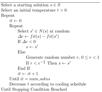
Simulated Annealing (Figure 5), first proposed by Kirkpatrick et al. [56], is similar to Hill Climbing in that it too attempts to improve one solution. However, Simulated Annealing attempts to escape local optima without the need to continually restart the search. It does this by tem-porarily accepting candidate solutions of poorer fitness, depending on the value of a variable known as the temperature. Initially the temperature is high, and free movement is allowed through the search space, with poorer neighbouring solutions representing potential moves along with better neighbouring solutions. As the search progresses, however, the temperature reduces, making moves to poorer solutions more and more unlikely. Eventually, freezing point is reached, and from this point on the search behaves identically to Hill Climbing. Pseudo-code for the Simulated Anneal-ing algorithm can be seen in Figure 6. The probability of acceptance p of an inferior solution is calculated as p=e−δt, where δ is the difference in fitness value between the current solution and the neighbouring inferior solution being considered, and tis the current value of the temperature control parameter.

‘Simulated Annealing’ is named so because it was inspired by the physical process of annealing; the cooling of a material in a heat bath. When a solid material is heated past its melting point and then cooled back into its solid state, the structural properties of the final material will vary depending on the rate of cooling.

F

itn

ess

Space of all possible solutions (a) A climb to a local optimum

F

itn

ess

Space of all possible solutions

(b) A restart resulting in a climb to the global optimum

Fig. 3.Hill Climbing seeks to improve a single solution, initially selected at random, by iteratively exploring its neighbourhood (adapted from McMinn [66])

Select a starting solutions∈S

Repeat

Selects0 ∈N(s) such thatf it(s0)> f it(s) according to ascent strategy

s←s0

Untilf it(s)≥f it(s0),∀s0 _∈N(s)

Fig. 4.High level description of a hill climbing algorithm, for a problem with solution spaceS; neighbour-hood structureN; andf it, the fitness function to be maximised (adapted from McMinn [65])

Hill Climbing and Simulated Annealing are said to belocal searches, because they operate with reference to one candidate solution at any one time, choosing ‘moves’ based on the neighbourhood of that candidate solution. Genetic Algorithms, on the other hand, are said to be global searches, sampling many points in the search space at once (Figure 7), offering more robustness to local optima. The set of candidate solutions currently under consideration is referred to as the current

population, with each successive population considered referred to as a generation. Genetic Algo-rithms are inspired by Darwinian Evolution, in keeping with this analogy, each candidate solution is represented as a vector of components referred to as individuals or chromosomes. Typically, a Genetic Algorithm uses a binary representation, i.e. candidate solutions are encoded as strings of 1s and 0s; yet more natural representations to the problem may also be used, for example a list of floating point values.

The main loop of a Genetic Algorithm can be seen in Figure 8. The first generation is made up of randomly selected chromosomes, although the population may also be ‘seeded’ with selected individuals representing some domain information about the problem, which may increase the chances of the search converging on a set of highly-fit candidate solutions. Each individual in the population is then evaluated for fitness.

On the basis of fitness evaluation, certain individuals are selected to go forward to the following stages of crossover, mutation and reinsertion into the next generation. Usually selection is biased towards the fitter individuals, however the possibility of selecting weak solutions is not removed so that the search does not converge early on a set of locally optimal solutions. The very first Genetic Algorithm, proposed by Holland4_{, used ‘fitness-proportionate’ selection, where the expected} number of times an individual is selected for reproduction is proportionate to the individual’s fitness in comparison with the rest of the population. However, fitness-proportionate selection has been criticised because highly-fit individuals appearing early in the progression of the search tend to dominate the selection process, leading the search to converge prematurely on one sub-area of the search space. Linear ranking [100] and tournament selection [23] have been proposed to circumvent these problems, involving algorithms where individuals are selected using relative rather than absolute fitness comparisons.

In the crossover stage, elements of each individual are recombined to form two offspring indi-viduals. Different choices of crossover operator are available, including ‘one-point’ crossover, which splices two parents at a randomly-chosen position in the string to form two offspring. For example, two strings ‘111’ and ‘000’ may be spliced at position 2 to form two children ‘100’ and ‘011’. Other operators may recombine using multiple crossover points, while ‘uniform’ crossover treats every position as a potential crossover point.

Subsequently, elements of the newly-created chromosomes are mutated at random, with the aim of diversifying the search into new areas of the search space. For GAs operating on binary representation, mutation usually involves randomly flipping bits of the chromosome. Finally, the next generation of the population is chosen in the ‘reinsertion’ phase, and the new individuals are evaluated for fitness. The GA continues in this loop until it finds a solution known to be globally optimal, or the resources allocated to it (typically a time limit or a certain budget of fitness evaluations) are exhausted. Whitley’s tutorial papers [101,102] offer a further excellent introductory material for getting starting with Genetic Algorithms in Search Based Software Engineering.

4 _{This was introduced by Holland [54], though Turing had also briefly mentioned the idea of evolution as} a computational metaphor [94].

F

itn

ess

Space of all possible solutions

Fig. 5.Simulated Annealing also seeks to improve a single solution, but moves may be made to points in the search space of poorer fitness (adapted from McMinn [66])

Select a starting solutions∈S

Select an initial temperaturet >0 Repeat it←0 Repeat Selects0∈N(s) at random ∆e←f it(s)−f it(s0) If∆e <0 s←s0 Else

Generate random number r, 0≤r <1 Ifr < e−δt Thens←s0

End If

it←it+ 1 Until it=num solns

Decrease taccording to cooling schedule Until Stopping Condition Reached

Fig. 6. High level description of a simulated annealing algorithm, for a problem with solution space S; neighbourhood structureN;num solns, the number of solutions to consider at each temperature level t; andf it, the fitness function to be maximised (adapted from McMinn [65])

F

itn

ess

Space of all possible solutions

Fig. 7.Genetic Algorithms are global searches, taking account of several points in the search space at once (adapted from McMinn [66])

Randomly generate or seed initial populationP

Repeat

Evaluate fitness of each individual inP

Select parents fromP according to selection mechanism Recombine parents to form new offspring

Construct new populationP0 from parents and offspring MutateP0

P ←P0

Until Stopping Condition Reached

5

Getting The First Result: A Simple Example for Regression Testing

This section presents an application of a search-based approach to the Test Case Prioritisation (TCP) in regression testing, illustrating the steps that are necessary to obtain the first set of results. This makes concrete the concepts of representation, fitness function and search based algorithm (and their operators) introduced in the previous sections. First, let us clarify what we mean by TCP.

Regression testing is a testing activity that is performed to gain confidence that the recent modifications to the System Under Test (SUT), e.g. bug patches or new features, did not interfere with existing functionalities [108]. The simplest way to ensure this is to execute all available tests; this is often called retest-all method. However, as the software evolves, the test suite grows too, eventually making it prohibitively expensive to adopt the retest-all approach. Many techniques have been developed to deal with the cost of regression testing.

Test Case Prioritisation represents a group of techniques that particularly deal with the permu-tations of tests in regression test suites [28, 108]. The assumption behind these techniques is that, because of the limited resources, it may not be possible to execute the entire regression test suite. The intuition behind Test Case Prioritisation techniques is that more important tests should be executed earlier. In the context of regression testing, the ‘important’ tests are the ones that detect regression faults. That is, the aim of Test Case Prioritisation is to maximiseearlier fault detection rate. More formally, it is defined as follows:

Definition 1 Test Case Prioritisation Problem

Given:a test suite,T, the set of permutations ofT,P T, and a function fromP T to real numbers,

f :P T →R.

Problem:to find T0∈P T such that (∀T00_)(T00_{∈P T)(T}00_6=T0_)[f(T0_)≥f(T00_)].

Ideally, the functionf should be a mapping from tests to their fault detection capability. How-ever, whether a test detects some faults or not is only known after its execution. In practice, a functionf that is a surrogate to the fault detection capability of tests is used. Structural coverage is one of the most popular choices: the permutation of tests that achieves structural coverage as early as possible is thought to maximise the chance of early fault detection.

5.1 Representation

At its core, TCP as a search problem is an optimisation in a permutation space similar to the Travelling Salesman Problem (TSP), for which many advanced representation schemes have been developed. Here we will focus on the most basic form of representation. The set of all possible candidate solutions is the set of all possible permutations of tests in the regression test suite. If the regression test suite contains n tests, the representation takes the form of a vector with n

elements. For example, Figure 9 shows one possible candidate solution for TCP with size n, i.e. with a regression test suite that contains 6 tests,{t0, . . . , t5}.

Depending on the choice of the search algorithm, the next step is either to define the neighbouring solutions of a given solution (local search) or to define the genetic operators (genetic algorithm).

t1 t3 t0 t2 t5 t4

Fig. 9.One possible candidate solution for TCP with a regression test suite with 6 tests,{t0, . . . , t5}.

Neighbouring Solutions Unless the characteristics of the search landscape is known, it is recom-mended that the neighbouring solutions of a given solution for a local search algorithm is generated by making the smallest possible changes to the given solution. This allows the human engineer to observe and understand the features of the search landscape.

It is also important to define the neighbouring solutions in a way that produces a manageable number of neighbours. For example, if the set of neighbouring solutions for TCP of sizenis defined as the set of all permutations that can be generated by swapping two tests, there would ben(n−

1) neighbouring solutions. However, if we only consider swapping adjacent tests, there would be

n−1. If the fitness evaluation is expensive, i.e. takes non-trivial time, controlling the size of the neighbourhood may affect the efficiency of the search algorithm significantly.

Genetic Operators The following is a set of simple genetic operators that can be defined over permutation-based representations.

– Selection:Selection operators tend to be relatively independent of the choice of representation. It is more closely related to the design of the fitness function. One widely used approach that is also recommended as the first step isn-way tournament selection. First, randomly samplen

solutions from the population. Out of this sample, pick the fittest individual solution. Repeat once again to select a pair of solutions for reproduction.

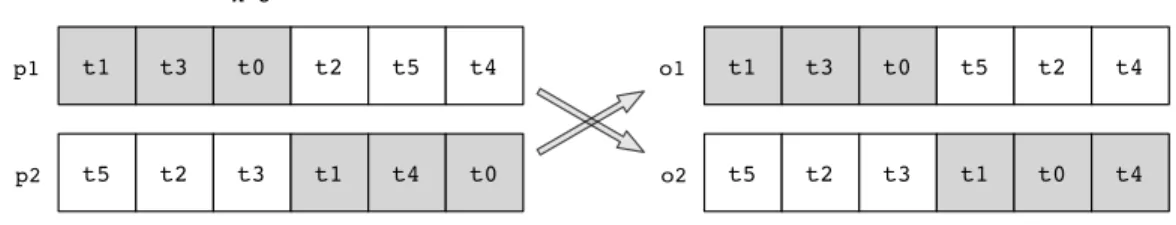
– Crossover:Unlike selection operators, crossover operators are directly linked to the structure of the representation of solutions. Here, we use the crossover operator following Antoniol et al. [6] to generate, from parent solutionsp1andp2, the offspring solutionso1 ando2:

1. Pick a random numberk(1≤k≤n)

2. The firstkelements ofp1 become the firstk elements ofo1.

3. The lastn−k elements ofo1 are the sequence of n−k elements that remain when the k elements selected fromp1are taken fromp2, as illustrated in Figure 10.

4. o2 is generated similarly, composed of the first n−k elements of p2 and the remaining k elements ofp1.

– Mutation:Similarly to defining the neighbouring solutions for local search algorithms, it is rec-ommended that, initially, mutation operators are defined to introduce relatively small changes to individual solutions. For example, we can swap the position of two randomly selected tests.

5.2 Fitness Function

The recommended first step to design the fitness function is to look for an existing metric that measures the quality we are optimising for. If one exists, it often provides not only a quick and easy way to evaluate the search-based approach to the problem but also a channel to compare the results to other existing techniques.

t1 t3 t0 t2 t5 t4 t5 t2 t3 t1 t4 t0 p1 p2 k=3 t1 t3 t0 t5 t2 t4 t5 t2 t3 t1 t0 t4 o1 o2

Fig. 10.Illustration of crossover operator for permutation-based representations following Antoniol et al.

The metric that is widely used to evaluate the effectiveness of TCP techniques is Average Percentage of Faults Detected (APFD) [28]. Higher APFD values mean that faults are detected earlier in testing. Suppose that, as the testing progresses, we plot the percentage of detected faults against the number of tests executed so far: intuitively, APFD would be the area behind the plot.

However, calculation of APFD requires the knowledge of which tests detected which faults. As explained in Section 5, the use of this knowledge defies the purpose of the prioritisation because fault detection information is not available until all tests are executed. This forces us to turn to the widely used surrogate, structural coverage. For example, Average Percentage of Blocks Covered (APBC) is calculated in a similar way to APFD but, instead of percentage of detected faults, percentage of blocks covered so far is used. In regression testing scenarios, the coverage information of tests are often available from the previous iteration of testing. While the recent modification that we are testing against might have made the existing coverage information imprecise, it is often

good enough to provide guidance for prioritisation, especially when regression testing is performed reasonably frequently.

5.3 Putting It All Together

The representation of solutions and the fitness function are the only problem-specific components in the overall architecture of SBSE approach in Figure 11. It is recommended that these problem specific components are clearly separated from the search algorithm itself: the separation not only makes it easier to reuse the search algorithms (that are problem independent) but also helps testing and debugging of the overall approach (repeatedly used implementations of search algorithms can provide higher assurance).

6

Understanding your results

6.1 Fair comparison

Due to the stochastic nature of optimisation algorithms, searches must be repeated several times in order to mitigate against the effects of random variation. In the literature, experiments are typically repeated 30-50 times.

When comparing two algorithms, the best fitness values obtained by the searches concerned are an obvious indicator to how well the optimisation process performed. However, in order to ensure a fair comparison, it is important to establish the amount of effort expended by each search

Representation Raw Data Fitness Function Metrics or Properties Search Algorithm

Fig. 11.Overall Architecture of SBSE Approach

algorithm, to find those solutions. This effort is commonly measured by logging thenumber of fitness evaluationsthat were performed. For example, it could be that an algorithm found a solution with a better fitness value, but did so because it was afforded a higher number of trials in which to obtain it. Or, there could be trade-offs, for example search A may find a solution of good fitness early in the search, but fail to improve it, yet searchB can find solutions of slightly better fitness, but requiring many more fitness evaluations in which to discover it. When a certain level of fitness is obtained by more than one search algorithm, theaverage number of fitness evaluationsover the different runs of the experiments by each algorithm is used to measure the cost of the algorithm in obtaining that fitness, or to put it another way, its relativeefficiency.

For some types of problem, e.g. test data generation, there is a specific goal that must be attained by the search; for example the discovery of test data to execute a particular branch. In such cases, merely ‘good’ solutions of high fitness are not enough - a solution with a certain very high fitness value must be obtained, or the goal of the search will not be attained. In such cases, best fitness is no longer as an important measure as thesuccess rate, a percentage reflecting the number of times the goal of the search was achieved over the repetitions of the experiment. The success rate gives an idea of how effectivethe search was at achieving its aim.

6.2 Elementary statistical analysis

The last section introduced somedescriptivestatistics for use in Search Based Software Engineering experiments, but alsoinferentialstatistics may be applied to discern whether one set of experiments are significantly different in some aspect from another.

Suppose there are two approaches to address a problem in SBSE, each of which involves the application of some search based algorithm to a set of problem instances. We collect results for the application of both algorithms,AandB, and we notice that, over a series of runs of our experiment, Algorithm Atends to perform better than Algorithm B. The performance we have in mind, may take many forms. It may be that Algorithm A is faster thanB, or that after a certain number of fitness evaluations it has achieved a higher fitness value, or a higher average fitness. Alternatively, there may be some other measurement that we can make about which we notice a difference in performance that we believe is worth reporting.

In such cases, SBSE researchers tend to rely on inferential statistics as a means of addressing the inherently stochastic nature of search based algorithms. That is, we may notice that the mean fitness achieved by Algorithm A is higher than that of Algorithm B after 10 executions of each,

but how can we besurethat this is not merely an observation arrived at bychance? It is to answer precisely these kinds of question that statistical hypothesis testing is used in the experimental sciences, and SBSE is no exception.

A complete explanation of the issues and techniques that can be used in applying inferential statistics in SBSE is beyond the scope of this tutorial. However, there has been a recent paper on the topic of statistical testing of randomised algorithms by Arcuri and Briand [8], which provides more detail. In this section we provide an overview of some of the key points of concern.

The typical scenario with which we are concerned is one in which we want to explore the likelihood that our experiments found that AlgorithmAoutperforms AlgorithmBpurely by chance. Usually we wish to be in a position to make a claim that we have evidence that suggests that Algorithm A is better than AlgorithmB. For example, as a sanity check, we may wish to show that our SBSE technique comfortably outperforms a random search. But what do we mean by ‘comfortably outperforms’ ?

In order to investigate this kind of question we set a threshold on the degree of chance that we find acceptable. Typically, in the experimental sciences, this level is chosen to be either 1% or 5%. That is, we will have either a less than 1 in 100 or a less than 5 in 100 chance of believing that Algorithm Aoutperforms AlgorithmB based on a set of executions when in fact it does not. This is the chance of making a so-called ‘Type I’ error. It would lead to us concluding that some AlgorithmAwas better than AlgorithmB when, in fact, it was not.

If we choose a threshold for error of 5% then we have a 95% confidence level in our conclusion based on our sample of the population of all possible executions of the algorithm. That is, we are ‘95% sure that we can claim that Algorithm A really is better than Algorithm B’. Unpacking this claim a little, what we find is that there is a population involved. This is the population of all possible runs of the algorithm in question. For each run we may get different behaviour due to the stochastic nature of the algorithm and so we are not in a position to say exactly what the value obtained will be. Rather, we can give a range of values.

However, it is almost always impractical to perform all possible runs and so we have to sample. Our ‘95% confidence claim’ is that we are 95% confident that the evidence provided by our sample allows us to infer a conclusion about the algorithm’s performance on the whole population. This is why this branch of statistics is referred to as ‘inferential statistics’; we inferproperties of a whole population based on a sample.

Unfortunately a great deal of ‘ritualistic’ behaviour has grown up around the experimental sciences, in part, resulting for an inadequate understanding of the underlying statistics. One aspect of this ritual is found in the choice of a suitable confidence level. If we are comparing some new SBSE approach to the state of the art, then we are asking a question as to whether the new approach is worthy of consideration. In such a situation we may be happy with a 1 in 10 chance of a Type I error (and could set the confidence level, accordingly, to be 90%). The consequences of considering a move from the status quo may not be so great.

However, if we are considering whether to use a potently fatal drug on a patient who may otherwise survive we might want a much higher confidence that the drug would, indeed, improve the health of the patent over the status quo (no treatment). For this reason it is important to think about what level of confidence is suitable for the problem in hand.

The statistical test we perform will result in ap-value. The p-value is the chance that a Type I error has occurred. That is, we notice that a sample of runs produces a higher mean result for a measurement of interest for AlgorithmA than for Algorithm B. We wish to reject the so-called ‘null hypothesis’; the hypothesis that the population of all executions of AlgorithmAis no different

to that of AlgorithmB. To do this we perform an inferential statistical test. If all the assumptions of the test are met and the sample of runs we have is unbiased then thep-value we obtain indicates the chance that the populations of runs of Algorithm A and AlgorithmB are identical given the evidence we have from the sample. For instance a p-value equal to or lower than 0.05 indicates that we have satisfied the traditional (and somewhat ritualistic) 95% confidence level test. More precisely, the chance of committing a Type I error isp.

This raises the question of how large a sample we should choose. The sample size is related to the statistical power of our experiment. If we have too small a sample then we may obtain high

p-values and incorrectly conclude that there is no significant difference between the two algorithms we are considering. This is a so-called Type II error; we incorrectly accept the null hypothesis when it is, in fact, false. In our case it would mean that we would incorrectly believe AlgorithmAto be no better than AlgorithmB. More precisely, we would conclude,correctly, that we have no evidence to claim that Algorithm Ais significantly better than AlgorithmB at the chosen conference level. However, had we chosen a larger sample, we may have had just such evidence. In general, all else being equal, the larger the sample we choose the less likely we are to commit a Type II error. This is why researchers prefer larger sample sizes where this is feasible.

There is another element of ritual for which some weariness is appropriate: the choice of a suitable statistical test. One of the most commonalty performed tests in work on search based algorithms in general (though not necessarily SBSE in particular) is the well-knownt test. Almost all statistical packages support it and it is often available at the touch of a button. Unfortunately, the t test makes assumptions about the distribution of the data. These assumptions may not be borne out in practice thereby increasing the chance of a Type I error. In some senses a type I error is worse than a Type II error, because it may lead to the publication of false claims, whereas a Type I error will most likely lead to researcher disappointment at the lack of evidence to support publishable results.

To address this potential problem with parametric inferential statistics SBSE researchers often use nonparametric statistical tests. Non-parametric tests make fewer assumptions about the distri-bution of the data. As such, these tests are weaker (they have less power) and may lead to the false acceptance of the null hypothesis for the same sample size (a Type II error), when used in place of a more powerful parametric test that is able to reject the null hypothesis. However, since the parametric tests make assumptions about the distribution, should these assumptions prove to be false, then the rejection of the null hypothesis by a parametric test may be an artefact of the false assumptions; a form of Type I error.

It is important to remember that all inferential statistical techniques are founded on probability theory. To the traditional computer scientist, particularly those raised on an intellectual diet con-sisting exclusively of formal methods and discrete mathematics, this reliance on probability may be as unsettling as quantum mechanics was to the traditional world of physics. However, as engineers, the reliance on a confidence level is little more than an acceptance of a certain ‘tolerance’ and is quite natural and acceptable.

This appreciation of the probability-theoretic foundations of inferential statistics rather than a merely ritualistic application of ‘prescribed tests’ is important if the researcher is to avoid mistakes. For example, armed with a non parametric test and a confidence internal of 95% the researcher may embark on a misguided ‘fishing expedition’ to find a variant of AlgorithmAthat outperforms AlgorithmB. Suppose 5 independent variants of AlgorithmAare experimented with and, on each occasion, a comparison is made with AlgorithmB using an inferential statistical test. If variant 3

produces a p-value of 0.05, while the others do not it would be a mistake to conclude that at the 95% confidence levelAlgorithm A (variant 3) is better than Algorithm B.

Rather, we would have to find that Algorithm A variant 3 had ap-value lower than 0.05/5; by repeating the same test 5 times, we raise the confidence required for each test from 0.05 to 0.01 to retain the same overall confidence. This is known as a ‘Bonferroni correction’. To see why it is necessary, suppose we have 20 variants of Algorithms A. What would be the expected likelihood that one of these would,by chance, have a p-value equal or lower than 0.05 in a world where none of the variants is, in fact, any different from AlgorithmB? If we repeat a statistical test sufficiently many times without a correction to the confidence level, then we are increasingly likely to commit a Type I error. This situation is amusingly captured by anxkcd cartoon [73].

Sometimes, we find ourselves comparing, not vales of measurements, but the success rates of searches. Comparison of success rates using inferential statistics requires a categorical approach, since a search goal is either fulfilled or not. For this Fisher’s Exact test is a useful statistical measure. This is another nonparametric test. For investigative of correlations, researchers use Spearman and Pearson correlation analysis. These tests can be useful to explore the degree to which increases in one factor are correlated to another, but it is important to understand that correlations does not, of course, entail causality.

7

More advanced techniques

Much has been achieved in SBSE using only a single fitness function, a simple representation of the problem and a simple search technique (such as hill climbing). It is recommended that, as a first exploration of SBSE, the first experiments should concern a single fitness function, a simple representation and a simple search technique. However, once results have been obtained and the approach is believed to have potential, for example, it is found to outperform random search, then it is natural to turn one’s attention to more advanced techniques and problem characterisations.

This section considers four exciting ways in which the initial set of results can be developed, using more advanced techniques that may better model the real world scenario and may also help to extend the range and type of results obtained and the applicability of the overall SBSE approach for the Software Engineering problem in hand.

7.1 Multiple Objectives

Though excellent results can be obtained with a single objective, many real world Software En-gineering problems are multiple objective problems. The objectives that have to be optimised are often in competition with one another and may be contradictory; we may find ourselves trying to balance the different optimisation objectives of several different goals.

One approach to handle such scenarios is the use of Pareto optimal SBSE, in which several optimisation objectives are combined, but without needing to decide which take precedence over the others. This approach is described in more detail elsewhere [48] and was first proposed as the ‘best’ way to handle multiple objectives for all SBSE problems by Harman in 2007 [36]. Since then, there has been a rapid uptake of Pareto optimal SBSE to requirements [27, 31, 84, 90, 113], planning [5,98], design [17,88,95], coding [9,99], testing [33,35,47,76,90,96,107], and refactoring [52]. Suppose a problem is to be solved that hasnfitness functions,f1, . . . , fn that take some vector

of parametersx. Pareto optimality combines a set of measurements,fi, into a single ordinal scale

F(x1)> F(x2)

⇔

∀i.fi(x1)≥fi(x2) ∧ ∃i.fi(x1)> fi(x2)

Under Pareto optimality, one solution is better than another if it is better according to at least one of the individual fitness functions and no worse according to all of the others. Under the Pareto interpretation of combined fitness, no overall fitness improvement occurs no matter how much almost all of the fitness functions improve, should they do so at the slightest expense of any one of their number. The use of Pareto optimality is an alternative to simply aggregating fitness using a weighted sum of thenfitness functions.

When searching for solutions to a problem using Pareto optimality, the search yields a set of solutions that are non–dominated. That is, each member of the non-dominated set is no worse than any of the others in the set, but also cannot be said to be better. Any set of non–dominated solutions forms a Pareto front.

Consider Figure 12, which depicts the computation of Pareto optimality for two imaginary fitness functions (Objective 1 and Objective 2). The longer the search algorithm is run the better the approximation becomes to the real Pareto front. In the figure, pointsS1,S2 andS3 lie on the Pareto front, whileS4 andS5 are dominated.

Fig. 12.Pareto Optimality and Pareto Fronts (taken from the survey by Harman et al. [48]).

Pareto optimality has many advantages. Should a single solution be required, then coefficients can be re-introduced in order to distinguish among the non–dominated set at the current Pareto front. However, by refusing to conflate the individual fitness functions into a single aggregate, the search may consider solutions that may be overlooked by search guided by aggregate fitness. The approximation of the Pareto front is also a useful analysis tool in itself. For example, it may contain ‘knee points’, where a small change in one fitness is accompanied by a large change in another. These knee points denote interesting parts of the solution space that warrant closer investigation.

7.2 Co Evolution

In Co–Evolutionary Computation, two or more populations of solutions evolve simultaneously with the fitness of each depending upon the current population of the other. Adamopoulos et al. [2] were the first to suggest the application of co-evolution to an SBSE problem, using it to evolve sets of mutants and sets of test cases, where the test cases act as predators and the mutants as their prey. Arcuri and Yao [10] use co-evolution to evolve programs and their test data from specifications using co-evolution.

Arcuri and Yao [11] also developed a co-evolutionary model of bug fixing, in which one population essentially seeks out patches that are able to pass test cases, while test cases can be produced from an oracle in an attempt to find the shortcomings of a current population of proposed patches. In this way the patch is the prey, while the test cases, once again, act as predators. The approach assumes the existence of a specification to act the oracle.

Many aspects of Software Engineering problems lend themselves to a co-evolutionary model of optimisation because software systems are complex and rich in potential populations that could be productively co-evolved (using both competitive and co-operative co-evolution). For example: components, agents, stakeholder behaviour models, designs, cognitive models, requirements, test cases, use cases and management plans are all important aspects of software systems for which optimisation is an important concern. Though all of these may not occur in the same system, they are all the subject of change. If a suitable fitness function be found, the SBSE can be used to co-evolve solutions.

Where two such populations are already being evolved in isolation using SBSE, but participate in the same overall software system, it would seem a logical ‘next step’, to seek to evolve these populations together; the fitness of one is likely to have an impact on the fitness of another, so evolution in isolation may not be capable of locating the best solutions.

7.3 SBSE as Decision Support

SBSE has been most widely used to find solutions to complex and demanding software engineering problems, such as sets of test data that meet test adequacy goals or sequences of transformations that refactor a program or modularisation boundaries that best balance the trade off between cohesion and coupling. However, in many other situations it is not the actual solutions found that are the most interesting nor the most important aspects of SBSE.

Rather, the value of the approach lies in the insight that is gained through the analysis inherent in the automated search process and the way in which its results capture properties of the structure of software engineering solutions. SBSE can be applied to situations in which the human will decide on the solution to be adopted, but the search process can provide insight to help guide the decision maker.

This insight agenda, in which SBSE is used to gain insights and to provide decision support to the software engineering decision maker has found natural resonance and applicability when used in the early aspects of the software engineering lifecycle, where the decisions made can have far–reaching implications.

For instance, addressing the need for negotiation and mediation in requirements engineering decision making, Finkelstein et al. [31] explored the use of different notions of fairness to explore the space of requirements assignments that can be said to be fair according to multiple definitions of ‘fairness’. Saliu and Ruhe [84] used a Pareto optimal approach to explore the balance of concerns between requirements at different levels of abstraction, while Zhang et al, showed how SBSE could be

used to explore the tradeoff among the different stakeholders in requirements assignment problems [112].

Many of the values used to define a problem for optimisation come from estimates. This is particularly the case in the early stages of the software engineering lifecycle, where the values available necessarily come from the estimates made by decision makers. In these situations it is not optimal solutions that the decision maker requires, so much as guidance on which of the estimates are most likely to affect the solutions. Ren et al. [46] used this observation to define an SBSE approach to requirements sensitivity analysis, in which the gaol is to identify the requirements and budgets for which the managers’ estimates of requirement cost and value have most impact. For these sensitive requirements and budgets, more care is required. In this way SBSE has been used as a way to provide sensitivity analysis, rather than necessarily providing a proposed set of requirement assignments.

Similarly, in project planning, the manager bases his or her decisions on estimates of work pack-age duration and these estimates are notoriously unreliable. Antoniol et al. [5] used this observation to explore the trade off between the completion time of a software project plan and the risk over overruns due to misestimation. This was a Pareto efficient, bi–objective approach, in which the two objectives were the completion time and the risk (measured in terms of overrun due to misestima-tion). Using their approach, Antoniol et al., demonstrated that a decision maker could identify safe budgets for which completion times could be more assured.

Though most of the work on decision support through SBSE has been conducted at the early stages of the lifecycle, there are still opportunities for using SBSE to gain insight at later stages in the lifecycle. For example, White et al. [99] used a bi-objective Pareto optimal approach to explore the trade off between power consumption and functionality, demonstrating that it was possible to find knee points on the Pareto front for which a small loss of functionality could result in a high degree of improved power efficiency.

As can be seen from these examples, SBSE is not merely a research programme in which one seeks to ‘solve’ software engineering problems; it is a rich source of insight and decision support. This is a research agenda for SBSE that Harman has developed through a series of keynotes and invited papers, suggesting SBSE as a source of additional insight and an approach to decision support for predictive modelling [38], cognitive aspects of program understanding [37], multiple objective regression testing [40] and program transformation and refactoring [41].

7.4 Augmenting with other non SBSE techniques

Often it is beneficial to augment search algorithms with other techniques, such as clustering or static analysis of source code. There is no hard rules for augmentation: different non-SBSE techniques can be considered appropriate depending on the context and challenge that are unique to the given software engineering problem. This section illustrates how some widely used non-SBSE techniques can help the SBSE approach.

Clustering Clustering is a process that partitions objects into different subsets so that objects in each group share common properties. The clustering criterion determines which properties are used to measure the commonality. It is often an effective way to reduce the size of the problem and, therefore, the size of the search space: objects in the same cluster can be replaced by a single representative object from the cluster, resulting in reduced problem size. It has been successfully applied when the human is in the loop [109].

Static Analysis For search-based test data generation approaches, it is common that the fitness evaluation involves the program source code. Various static analysis techniques can improve the ef-fectiveness and the efficiency of code-related SBSE techniques. Program slicing has been successfully used to reduce the search space for automated test data generation [43]. Program transformation techniques have been applied so that search-based test data generation techniques can cope with flag variables [15].

Hybridisation While hybridising different search algorithms are certainly possible, hybridisation with non-SBSE techniques can also be beneficial. Greedy approximation has been used to inject

solutions into MOEA so that MOEA can reach the region close to the true Pareto front much faster [107]. Some of more sophisticated forms of hybridisation use non-SBSE techniques as part of fitness evaluation [105].

8

Case studies

This section introduces four case studies to provide the reader with a range of examples of SBSE application in software engineering. The case studies are chosen to represent a wide range of topics, illustrating the way in which SBSE is highly applicable to Software Engineering problem; with just a suitable representation, fitness function and a choice of algorithm it is possible to apply SBSE to the full spectrum of SBSE activities and problems and to obtain interesting and potentially valuable results. The case studies cover early lifecycle activities such as effort estimation and re-quirements assignment through test case generation to regression testing, exemplifying the breadth of applications to which SBSE has already been put.

8.1 Case Study: Multi-Objective Test Suite Minimisation

Let us consider another class of regression testing techniques that is different from Test Case Prioritisation studied in Section 5: test suite minimisation. Prioritisation techniques aim to generate an ideal test execution order; minimisation techniques aim to reduce the size of the regression test suite when the regression test suite of an existing software system grows to such an extent that it may no longer be feasible to execute the entire test suite [80]. In order to reduce the size of the test suite, anyredundant test cases in the test suite need to be identified and removed.

Regression Testing requires optimisation because of the problem posed by large data sets. That is, organisations with good testing policies quickly accrue large pools of test data. For example, one of the regression test suites studied in this paper is also used for a smoke-test by IBM for one of its middleware products and takes over 4 hours if executed in its entirety. However, a typical smoke-test can be allocated only 1 hour maximum, forcing the engineer either to select a set of test cases from the available pool or to prioritise the order in which the test cases are considered.

The cost of this selection or prioritisation may not be amortised if the engineer wants to apply the process with every iteration in order to reflect the most recent test history or to use the whole test suite more evenly. However, without optimisation, the engineer will simply run out of time to complete the task. As a result, the engineer may have failed to execute the most optimal set of test cases when time runs out, reducing fault detection capabilities and thereby harming the effectiveness of the smoke test.

One widely accepted criterion for redundancy is defined in relation to the coverage achieved by test cases [16, 20, 53, 74, 81]. If the test coverage achieved by test case t1 is a subset of the test

coverage achieved by test caset2, it can be said that the execution oft1is redundant as long ast2is also executed. The aim of test suite minimisation is to obtain the smallest subset of test cases that are not redundant with respect to a set of test requirements. More formally, test suite minimisation problem can be defined as follows [108]:

Definition 2 Test Suite Minimisation Problem

Given:A test suite of ntests,T, a set ofm test goals{r1, . . . , rm}, that must be satisfied to

pro-vide the desired ‘adequate’ testing of the program, and subsets of T,Tis, one associated with each

of theris such that any one of the test casestj belonging toTican be used to achieve requirementri.

Problem: Find a representative set,T0, of test cases from T that satisfies allris.

The testing criterion is satisfied when every test-case requirement in{r1, . . . , rm}is satisfied. A

test-case requirement,ri, is satisfied by any test case,tj, that belongs toTi, a subset ofT. Therefore,

the representative set of test cases is the hitting set of Tis. Furthermore, in order to maximise the

effect of minimisation,T0should be the minimal hitting set ofTis. The minimal hitting-set problem

is an NP-complete problem as is the dual problem of the minimal set cover problem [34].

The NP-hardness of the problem encouraged the use of heuristics and meta-heuristics. The greedy approach [74] as well as other heuristics for minimal hitting set and set cover problem [20,53] have been applied to test suite minimisation but these approaches were not cost-cognisant and only dealt with a single objective (test coverage). With the single-objective problem formulation, the solution to the test suite minimisation problem is one subset of test cases that maximises the test coverage with minimum redundancy.

Later, the problem was reformulated as a multi-objective optimisation problem [106]. Since the greedy algorithm does not cope with multiple objectives very well, Multi-Objective Evolutionary Algorithms (MOEAs) have been applied to the multi-objective formulation of the test suite minimi-sation [63, 106]. The case study presents the multi-objective formulation of test suite minimiminimi-sation introduced by Yoo and Harman [106].

Representation Test suite minimisation is at its core a set-cover problem; the main decision is whether to include a specific test into the minimised subset or not. Therefore, we use the binary string representation. For a test suite withntests,{t1, . . . , tn}, the representation is a binary string

of lengthn: thei-th digit is 1 iftiis to be included in the subset and 0 otherwise. Binary tournament

selection, single-point crossover and single bit-flip mutation genetic operators were used for MOEAs.

Fitness Function Three different objectives were considered: structural coverage, fault history coverage and execution cost. Structural coverage of a given candidate solution is simply the struc-tural coverage achieved collectively by all the tests that are selected by the candidate solution (i.e. their corresponding bits are set to 1). This information is often available from the previous iteration of regression testing. This objective is to be maximised.

Fault history coverage is included to compliment structural coverage metric because achieving coverage may not always increase fault detection capability. We collect all known previous faults and calculatefault coveragefor each candidate solution by counting how many of the previous faults

could have been detected by the candidate solution. The underlying assumption is that a test that has detected faults in the past may have a higher chance of detecting faults in the new version. This objective is to be maximised.

The final objective is execution cost. Without considering the cost, the simplest way to maximise the other two objectives is to select the entire test suite. By trying to optimise for the cost, it is possible to obtain the trade-off between structural/fault history coverage and the cost of achieving them. The execution cost of each test is measured using a widely-used profiling tool calledvalgrind.

Algorithm A well known MOEA by Deb et al. [24], NSGA-II, was used for the case study. Pareto optimality is used in the process of selecting individuals. This leads to the problem of selecting one individual out of a non-dominated pair. NSGA-II uses the concept of crowding distance to make this decision; crowding distance measures how far away an individual is from the rest of the population. NSGA-II tries to achieve a wider Pareto frontier by selecting individuals that are far from the others. NSGA-II is based on elitism; it performs the non-dominated sorting in each generation in order to preserve the individuals on the current Pareto frontier into the next generation.

The widely used single-objective approximation for set cover problem is greedy algorithm. The only way to deal with the chosen three objectives is to take the weighted sum of each coverage metric per time, i.e.:

Fig. 13. A plot of 3-dimensional Pareto-front from multi-objective test suite minimisation for program spacefrom European Space Agency, taken from Yoo and Harman [106].

Results Figure 13 shows the results for the three objective test suite minimisation for a test suite of a program calledspace, which is taken from Software Infrastructure Repository (SIR). The 3D

plots display the solutions produced by the weighted-sum additional greedy algorithm (depicted by + symbols connected with a line), and the reference Pareto front (depicted by × symbols). The reference Pareto front contains all non-dominated solutions from the combined results of weighted-sum greedy approach and NSGA-II approach. While the weighted-weighted-sum greedy approach produces solutions that are not dominated, it can be seen that NSGA-II produces a much richer set of solutions that explore wider area of the trade-off surface.

8.2 Case Study: Requirements Analysis

Selecting a set of software requirements for the release of the next version of a software system is a demanding decision procedure. The problem of choosing the optimal set of requirements to include in the next release of a software system has become known as the Next Release Problem (NRP) [13, 113] and the activity of planning for requirement inclusion and exclusion has become known as release planning [82, 84].

The NRP deals with the selecting a subset of requirements based on their desirability (e.g. the expected revenue) while subject to constraints such as a limited budget [13]. The original formulation of NRP by Bagnall et al. [13] considered maximising the customer satisfaction (by inclusion of their demanded requirements in the next version) while not exceeding the company’s budget.

More formally, let C ={c1, . . . , cm} be the set of m customers whose requirements are to be

considered for the next release. The set of n possible software requirements is denoted by R =

{r1, . . . , rn}. It is assumed that all requirements are independent, i.e. no requirement depends on

others5_{. Finally, let cost= [cost}

1, . . . , costn] be the cost vector for the requirements inR:costi is

the associate cost to fulfil the requirementri.

We also assume that each customer has a degree of importance for the company. The set of relative weights associated with each customer cj(1 ≤j ≤m) is denoted byW ={w1, . . . , wm},

where wj ∈ [0,1] and P m

j=1wj = 1. Finally, it is assumed that all requirements are not equally

important for a given customer. The level of satisfaction for a given customer depends on the requirements that are satisfied in the next release of the software. Each customer cj(1≤j ≤m)

assigns a value to requirement ri(1 ≤ i ≤n) denoted by value(ri, cj) where value(ri, cj) >0 if

customercj gets the requirementri and 0 otherwise.

Based on above, the overallscore, or importance of a given requirementri(1≤i≤n), can be

calculated as scorei =P m

j=1wj·value(ri, cj). The score of a given requirement is represented as

its overallvalue to the organisation.

The aim of the Multi-Objective NRP (MONRP) is to investigate the trade-off between the score and cost of requirements. Letscore= [score1, . . . , scoren] be the score vector calculated as above.

Letx= [x1, . . . , xn]∈ {0,1}n a solution vector, i.e. a binary string identifying a subset ofR. Then

MONRP is defined as follows:

Definition 3 Given: The cost vector, cost = [cost1, . . . , costn] and the score vector (calculated

from the customer weights and customer-assigned value of requirements)score= [score1, . . . , scoren].

Problem: MaximisePn

i=1scorei·xi while minimisingP n

i=1costi·xi.

5 _{Bagnall et al. [13] describe a method to remove dependences in this context by computing the transitive} closure of the dependency graph and regarding each requirement and all its prerequisites as a new single requirement.

Representation Similar to the test suite minimisation problem in Section 8.1, the candidate solution for NRP should denote whether each requirement will beselected, i.e. implemented in the next release. For a set ofnrequirements,{r1, . . . , rn}, a candidate solution can be represented with

a binary string of lengthn: thei-th digit is 1 ifri is to be included in the subset and 0 otherwise.

Fitness Function Thecost and profit function can be directly used as fitness functions for each objectives for MOEAs:cost should be minimised while profit should be maximised.

Algorithm The case study compares three different evolutionary algorithms to random search: NSGA-II, Pareto-GA and a objective GA. Pareto-GA is a variation of a generic single-objective GA that uses Pareto-optimality only for the selection process. The single-single-objective GA is used to deal with the multi-objective formulation of NRP by adopting different sets of weights with the weighted-sum approach. When using weighted-sum approach for two objective functions,

f1 andf2, the overall fitness F of a candidate solutionxis calculated as follows:

F(x) =w·f1(x) + (1−w)·f2(x)

Depending on the value of the weight,w, the optimisation will target different regions on the Pareto front. The case study considered 9 different weight values ranging from 0.1 to 0.9 with step size of 0.1 to achieve wider Pareto fronts.

0 2000 4000 6000 8000 10000 12000 14000 −180 −160 −140 −120 −100 −80 −60 −40 −20 0 Score − 1*Cost NSGA−II Pareto GA Random search Single−Objective GA 0 5000 10000 15000 −80 −70 −60 −50 −40 −30 −20 −10 0 Score − 1*Cost NSGA−II Pareto GA Random search Single−Objective GA

(a) 15 customers; 40 requirements (d) 100 customers; 20 requirements

0 0.5 1 1.5 2 x 105 −400 −350 −300 −250 −200 −150 −100 −50 0 Score − 1*Cost NSGA−II Pareto GA Random search Single−Objective GA 0 0.5 1 1.5 2 2.5 3 3.5 4 4.5 x 104 −140 −120 −100 −80 −60 −40 −20 0 Score − 1*Cost NSGA−II Pareto GA Random search Single−Objective GA

(b) 50 customers; 80 requirements (e) 100 customers; 25 requirements

0 2 4 6 8 10 12 x 105 −550 −500 −450 −400 −350 −300 −250 −200 −150 −100 −50 0 Score − 1*Cost NSGA−II Pareto GA Random search Single−Objective GA 1 1.5 2 2.5 3 x 104 −800 −700 −600 −500 −400 −300 −200 −100 Score − 1*Cost NSGA−II Pareto GA Random search Single−Objective GA

(c) 100 customers; 140 requirements (f) 2 customers; 200 requirements

Figure 1: In (a), (b) and (c) metaheuristic search techniques have outperformed Random Search. The NSGA-II performed better or equal to others for a large part of the Pareto front while Single-Objective performed better in the extreme regions. The gap between search techniques and Random Search became larger as the problem size increased. (d) shows the boundary case concerning the number of requirements beyond which, Random Search fails to produce comparable results with metaheuristic search techniques. (e) shows 25% increase in the number of requirements, the gap became significant. The NSGA-II performed the best, and Pareto GA shared part of the front with NSGA-II. (f ) shows that the gap was obviously large. The NSGA-II has outperformed Pareto GA but not the Single-Objective GA in the extreme ends of the front.