Sharif University of Technology
Scientia IranicaTransactions E: Industrial Engineering www.scientiairanica.com
Integrated production and distribution scheduling for
perishable products
F. Marandi and S.H. Zegordi
Department of Industrial Engineering, Tarbiat Modares University, Tehran, Iran.
Received 20 October 2015; received in revised form 18 April 2016; accepted 5 December 2016
KEYWORDS Production and distribution;
Permutation ow shop scheduling;
Vehicle routing problem; Integration; Mixed integer programming; Particle swarm optimization.
Abstract. This study is concerned with how the quality of perishable products can be improved by shortening the time interval between production and distribution. Since special types of food, such as dairy products, decay fast, the Integration of Production and Distribution Scheduling (IPDS), is investigated. This article deals with a variation of IPDS that contains a short shelf life product; hence, there is no inventory of the product in the process. Once a specic amount of the product is produced, it must be transported with the least transportation time directly to various customer positions within its limited lifespans to minimize the delivery and tardy costs required to complete producing and distributing of the product to satisfy the demand of customers within the limited deadline. After developing a mixed-integer nonlinear programming model of the problem, because it is NP-hard, an Improved Particle Swarm Optimization (IPSO) is proposed. IPSO performance is compared with commercial optimization software for small-size and moderate-size problems. For large-size ones, it is compared with the genetic algorithm existing in the literature. Computational experiments show the eciency and eectiveness of the proposed IPSO in terms of both the quality of the solution and the time of achieving the best solution.
© 2017 Sharif University of Technology. All rights reserved.
1. Introduction
Production and distribution operations are two impor-tant operational functions in a supply chain. To achieve optimal operational performance in a supply chain, it is signicant to integrate these two functions and schedule them jointly in a coordinated manner. However, most of the proposed integrated and synchronized approaches focus on the tactical decision level of supply chains [1,2]. In recent years, integrated scheduling has attracted much interest among researchers. In contrast to classical scheduling, this type of schedul-ing problem involves not only the production part but also distribution. The objective of integrated scheduling is to obtain a simultaneous optimization
*. Corresponding author. Tel.: +98 21 82883394 E-mail address: [email protected] (S.H. Zegordi)
of both parts. The obtained procedure will become a detailed schedule that provides an ecient solution for operation management. In this paper, a class of integrated scheduling problems is considered, which includes production and distribution.
In many applications involving make-to-order or time-sensitive (e.g., perishable) products, nished or-ders are often delivered to customers immediately or shortly after the production to restrict quality reduction. In such a supply chain, product quality is determined not only by the production processes but also through the coordination of the production and distribution decisions. In this situation, the delivery of the products must be done within a strictly limited time after their production. The non-inventory pro-duction and transportation problem is routine in many industries, in which a time-sensitive product cannot be in storage due to its short shelf life. The delivery of
the product must be made within a tightly limited time after its production. Therefore, the production and dis-tribution operations must be highly integrated. When the production plant has a limited production rate and the transportation time is not instantaneous, any ineciency in the integrated schedule may either cause the product to expire before it reaches the customers or cause the delivery not to satisfy a customer's delivery deadline. Then, the production and distribution oper-ations must be highly linked and integrated because any ineciency in the integrated schedule causes a decrease in product quality, expiration before delivery, extra expenses, and lack of customer satisfaction. To ease this coordination, production sites are usually directly connected to customers by a eet of vehicles [3]. Consequently, there is little or no nished product inventory in the supply chain such that production and outbound distribution are very closely linked, which must be scheduled jointly in order to achieve a desired on-time delivery performance at a minimum total cost. However, the analysis of practices in case studies show that, currently, the production and distribution operations are done separately, which cause operational and customer dissatisfaction [4]. Thus, this paper investigates integrating production and distribution decisions at a trade-o among customer satisfaction, quality of delivered products, and total costs. Research on integrated scheduling models of production and distribution is relatively new, but it is growing very rapidly.
This study was motivated by a practical schedul-ing problem encountered by a leadschedul-ing manufacturer of various industries, in which a limited number of vehicles were available, where the departure time after production in owshop scheduling was not xed and needed to be determined in order to minimize tardy and delivery costs to satisfy the customers' deadline. The dierences and contributions of this paper compared with IPDS's literature can be summarized as follows:
1. A new problem is dened. The Integrated Production-Distribution Scheduling (IPDS) prob-lem is considered, of which the rst stage con-tains permutation ow shop scheduling and the second stage involves the distribution problem that requires designing vehicle routes for picking up nished goods and delivering them from the manu-facturer to customers;
2. A new mixed integer nonlinear programming model is developed, which simultaneously considers both production and distribution scheduling in an inte-grated manner. The exact solution to the problem is provided by solving the model. This model is practical in large scales for real cases, such as the dairy product industry, which is motivated by a case study from a dairy manufacturer in Tehran;
3. An Improved Particle Swarm Optimization (IPSO) is proposed to deal with the problem. The improv-ing operator, 1-exchanged and 2-opt, is added to prevent premature convergence;
4. New test problems are created, which can be used for future studies.
This paper studies the integrated production and dis-tribution scheduling problem and extends features such as non-negligible transportation time and delivery con-solidation. Comparison of this problem with previous works shows the combination of the product's limited lifespan, machine scheduling decisions, and the vehicle routing decisions as critical features that make it dier-ent, which leads to the possibility of expiration before it reaches a customer. The problem is complicated by limited transportation capacity, a customer's demand size and location, and the departure time that must be determined and are not xed. On the other hand, these complications also make the resulting integrated scheduling problem challenging and interesting. The particular variation that is considered involves a single production plant with multiple production machines in owshop scheduling, a eet of delivery trucks, and a given set of customers at dierent locations over a geographic region.
The aim of this research is integrating scheduling in a mathematical model, which is developed to in-vestigate the eect of integrated production scheduling and distribution decisions on the total costs. This is similar to various real-world environments such as food, dairy products, and chemical industries, which are highly perishable. Since this problem has an NP-hard structure [5], a meta-heuristic method is used to solve it. An Improved Particle Swarm Optimization (IPSO) is proposed in this study that improves the operator, while 1-exchanged and 2-opt is added to prevent premature convergence.
The remainder of this paper is organized as follows. Section 2 presents results from previous works on integrated supply chain scheduling. In Section 3, the problem is described and the mathematical model of the problem is presented. In Section 4, an improved particle swarm optimization is proposed to solve the problem. In Section 5, the experimental results of the proposed IPSO and managerial implications are presented. At the end, Section 6 elaborates concluding remarks and some suggestions for future research.
2. Literature review
In this section, the literature that explicitly involves both production and transportation activities in in-tegrated supply chain scheduling is presented. Inte-grating production and outbound delivery scheduling is very critical and common in the supply chain of
time-sensitive products [6,7]. For example, Buer et al. [8] focus on the newspapers printing and distribution, and mail processing and distribution provided by Wang et al. [9], and industrial adhesive materials produc-tion and delivery provided by Devapriya et al. [10]. Therefore, how to eectively integrate the production and delivery stages at the operational level so as to decrease the operational costs and improve customer service becomes very important for the success of a company. However, most of the existing models on the production-distribution scheduling problems only study strategic or tactical levels of decisions, and very few have addressed integrated decisions at the operational level. Chandra and Fisher [11] emphasize the need for studying these integrated scheduling issues at the operational level. They consider an integrated scheduling problem where a plant produces and stores the products until they are delivered to the customers by a eet of trucks. They provide two solutions. The rst solution solves the production scheduling and vehicle routing problems, separately, but the second one solves the problem in a coordinated manner. Their computational results show that the total operating cost decreases in the coordinated one. Chen and Vairaktarakis [12] and Pundoor and Chen [13] also show that there is signicant benet by using the optimally integrated production-distribution schedule compared to the schedule generated by a separate and sequential scheduling approach in the context of the models that are considered in their research. They emphasize that integration is a prior approach to improve the total performance in decreasing costs that is investigated in this paper.
Chen [6,14] reviews papers that deal with in-tegrated production scheduling and outbound distri-bution. He focuses on two main areas of direct delivery (one destination) and vehicle routing (multi destinations). He also provides a survey of models and results in the area of integrated scheduling of production and distribution. He presents a unied model representation scheme, classies existing models into several dierent classes, and, for each class of the models, gives an overview of the optimality properties, computational tractability, and solution algorithms for the various problems studied in the literature. In his survey on the relevant literature, he states that although there is a huge amount of research on integrated production and distribution models, the need for focusing on more studies in this realm is required. In his research, he notes a gap in the consideration of a due date and distribution by vehicle routing for practical situations. Lee and Chen [15] study the machine scheduling problems with explicit transportation considerations. They identify two types of transportation situations in their models. The rst type involves transporting a semi-nished job from one
machine to another for further processing. The second type involves transporting a nished job to the cus-tomer or warehouse. Both transportation capacity and transportation time are taken into account explicitly in their model. They classify the computational complex-ity of various scheduling problems by either proving their NP-hardness or providing polynomial algorithms. Chang and Lee [5] consider an extension of Lee and Chen's work where each job is assumed to occupy a dierent amount of storage space in the vehicle during delivery. They show the problem that jointly considers production and delivery with the consideration that each job may require a dierent amount of space during intractable transport and provide heuristics for some cases of the problem. Zhong et al. [16] study the similar problem as the one studied by [5] with the objective of minimizing the makespan. In the practical cases, focusing on the type of transportation, Hajiaghaei-Keshteli and Aminnayeri [17] present inte-grated production and rail transportation scheduling by emphasizing the application of rail distribution. Saidi-Mehrabad et al. [18] present a new integrated model in scheduling and routing by automated guided vehicles that focus on new methods of transportation. In some research, the types of products are more important than the types of transportation in practical models investigated in integrated modelling. Chen et al. [19] and Farahani et al. [3] propose a production and distribution scheduling for perishable food products. Liu et al. [20] present an integrated scheduling to improve the operation of production and delivery in ready-mixed concrete plants. Algorithms for solving these problems include approximation algorithms [21] and intelligent algorithms [4,22,23]. As mentioned, the type of product and transportation is important in practical cases and industries that is emphasized in this paper, as follows.
To the best of our knowledge, it seems that no research considers both permutation ow shop scheduling with due date and tardy cost in the pro-duction stage, and vehicle routing with consideration of deadline to satisfy customers. Few studies consider the transportation eet in their models. This study is extended by assuming that the rst stage of the supply chain is composed of m machines as the ow shop environment in the production stage, and v vehicles involved in designing vehicle routes for picking up and delivering nished goods in the second stage. It can be practical in real cases to serve a number of customers in various geographical zones.
3. Problem description 3.1. Assumptions
As mentioned previously, the scheduling of products and vehicles in a two-stage supply chain is investigated
here. The rst stage contains permutation ow shop scheduling with m machines and n jobs, and the second stage is composed of v vehicles with dierent speeds and transportation capacities that transport n jobs from the manufacturing company to c customers distributed in various geographical zones. All vehicles are available upon completion of all jobs (i.e., Cmax).
The problem is described as follows. There is a set of jobs (N = f1; 2; ; ng) to be processed by a set of machines (M = f1; 2; ; mg) at the production stage, which is permutation ow shop scheduling. All jobs have to be processed in an identical order on a given set of machines. The processing of each job is continuous once the processing begins. After processing, the nished jobs need to be delivered by a set of vehicles, V = f1; 2; ; vg, which has a distinct capacity, Qk,
to a set of customers, C = f1; 2; ; cg, that aims to nd a set of tours for several vehicles from a depot (i.e. manufacturer site) to a lot of customers. They return to the depot without exceeding capacity and deadline constraints. Each customer is visited only once by a single vehicle. Delay is not allowed, i.e. the jobs have to be delivered to the customers before the deadline. Moreover, when the last job terminates (i.e., makespan) after the due date, it will incur the tardy cost. The objective is to nd an integrated production and distribution to minimize the sum of jobs' delivery cost and tardy cost that refers to the due date violation.
At the beginning of the horizon, customers re-quire a set of jobs and send the rere-quirements to the manufacturer. At the subsequent delivery stage, a eet of capacitated vehicles delivers the nished jobs to the pre-specied customers. The capacity of the transporter is measured by a certain volume. Each customer is visited only once by a single vehicle. Only one vehicle is allowed to visit each customer.
3.2. Mathematical model
A mathematical formulation of the proposed Integrated Production-Distribution Scheduling (IPDS) problem is presented in this section. The parameters are as follows:
n Number of jobs m Number of machines c Number of customers v Number of vehicles i Job index, i = 1; 2; ; n
p Job position index, p = 1; 2; ; n r Machine index, r = 1; 2; ; m j; l Customer index
k Vehicle index vk Speed of vehicle k
Tri Operation time of job i on machine r
djl Distance between customer j and
customer l
eij Physical space of customer j's demand
i
ddk Deadline for vehicle k to deliver to
customers
Qk Capacity of vehicle k for transporting
job from manufacturing company to customers
du Due date for production stage cd Transportation cost per unit of
distance
cp Violation due date cost in production stage
M A suciently large number Variables of the model are as follows: Brj Start time of job j on machine r
uj Number of customers visited at
customer j
rk Ready time of vehicle k representing
the latest completion time
cmax Maximum completion time of all jobs
(makespan)
zij 1 if job i in position j is processed;
zero otherwise xk
jl 1 if customer l is served after customer
j by vehicle k; zero otherwise y 1 if cmax is after due date; zero
otherwise
Miller et al. [24] propose a mathematical pro-gramming formulation to prevent sub-tours in the vehicle routing problem. Kyparisis and Koulamas [25] propose a denition to consider the vehicle velocity and distance instead of time. All the above assumptions are used to develop the following model for the Integrated Production-Distribution Scheduling (IPDS) problem:
Min cdXv
k=1 c
X
l=0 c
X
j=0
dljxklj+ cp:y(cmax du);
n
X
p=1
Zip= 1 1 i n; (1)
n
X
i=1
Zip= 1 1 p n; (2)
B1p+ n
X
i=1
T1iZip= B1;p+1 1 p n 1; (3)
Br1+ n
X
i=1
TriZi1= Br+1;1 1 r m 1; (5)
Brp+ n
X
i=1
TriZip Br+1;p
1 r m 1 2 p n; (6)
Brp+ n
X
i=1
TriZip Br;p+1
1 p n 1 2 r m; (7)
cmax= Bmn+ n
X
i=1
TmiZin; (8)
v X k=1 c X l=1 xk
jl= 1 j = 1; 2; ; c; (9) v X k=1 c X j=1 xk
jl= 1 l = 1; 2; ; c; (10) c X l=0 xk lh c X j=0 xk hj= 0
k = 1; 2; ; v; h = 1; 2; ; c; (11)
c
X
j=1
xk
0j= 1; k = 1; 2; ; v; (12)
uj+ 1 ul+ c(1 xkjl) k = 1; 2; ; v;
l = 1; 2; ; c; j = 1; 2; ; c; (13)
v X k=1 c X j=1 xk
0j= v; (14)
v X k=1 c X l=1 xk
l0= v; (15)
n X i=1 c X j=0 c X l=0
eijxklj Qk k = 1; 2; ; v; (16)
rk c
max k = 1; 2; ; v; (17)
rk+Xc l=1
c
X
j=0
djl=vkxkjl ddk k = 1; 2; ; v;
(18) cmax du M(1 y); (19)
cmax du + My: (20)
The aim is to minimize the sum of delivery and tardy
costs. Constraint sets (1) and (2) represent the assign-ment that guarantees to assign every job to one position and every position to one job. Constraint sets (3)-(5) ensure the permutation ow shop scheduling property in which there is no idle time on the rst machine and the rst job is processed on all machines without delay. Constraint set (6) guarantees that the start of each job on machine r + 1 is not earlier than its nish time on machine r, which prevents the simultaneous processing of jobs on one machine. Constraint set (7) ensures that the job processes in position p + 1 in the sequence do not start until the processing of the job in position p on that machine is completed. Constraint set (8) represents makespan. Constraint sets (9) and (10) are common constraints for the vehicle routing problem that causes every customer to be serviced by only one vehicle. Constraint set (11) is the ow conservation constraint for each customer and when the vehicle serves the customer, it must depart the current customer to service the next ones. Constraint set (12) ensures that every vehicle must serve the customer once. Constraint set (13) prevents the sub tour that is disconnected to the depot. Constraint sets (14) and (15) conne the number of vehicles to serve the customers to v vehicles. Constraint set (16) guarantees that the maximum ow in any arc leaving the root is equal to Qk and the maximum
vehicle k capacity is conned to Qk. The relation of
the production and distribution stages is important in the IPDS problem. Constraint set (17) focuses on integration of the production and distribution stages, which emphasizes the ready time of vehicles upon completion of all jobs. Constraint set (18) focuses on satisfying the deadline to serve the customer in order to increase customer satisfaction. Constraint sets (19) and (20) determine variable y to get 1 or 0 that is dependent on makespan violation of the due date.
It should be mentioned that as the objective function contains non-linear terms, the mathematical model is a Mixed-Integer Non-Linear Programming (MINLP) model. The model could be solved with commercial software packages such as LINGO.
Lemma 1. The Integrated Production-Distribution Scheduling (IPDS) problem is NP-hard.
Proof. Chang and Lee [5] proved a problem with only one geographical zone, one manufacturer, and one vehicle as NP-hard. According to [26,27], the ow shop scheduling problem with Cmax minimization objective
is also NP-hard. As the IPDS problem is an extension of two NP-hard problems, i.e. the ow shop scheduling and vehicle routing problem, the integrated problem must be NP-hard in the strong sense.
NP is not equal to P problems, so there is no algorithm to nd global optima in polynomial compu-tational time. Therefore, meta-heuristics or heuristics must be applied to solve large-scale problems within reasonable computation time. After introducing the particle swarm optimization algorithm, the improved algorithm, IPSO, is proposed in Section 4. In Section 5, it is validated by the generated test problems.
4. Meta-heuristic algorithms
Each of the integrated production and distribution scheduling problems is strongly NP-hard [4,5]. There-fore, an Improved Particle Swarm Optimization is proposed to deal with the proposed problem in this research. For validation of IPSO, a genetic algorithm emanated by [4] is applied.
4.1. Improved Particle Swarm Optimization (IPSO)
Various approaches have been proposed to solve scheduling problems. Among them, PSOs have been greatly adopted during recent years in practical do-mains [28,29]. The Particle Swarm Optimization (PSO) is a population-based optimization algorithm based on the benchmarking of social interactions such as bird ocking or sh school. It is developed by [30] in which the members of the whole population are maintained through the search procedure, so that information is socially shared among individuals to guide the search towards the best position in the search space. PSO is an evolutionary algorithm, which is ini-tialized with a population (swarm) of random solutions (particles) that y in the search space. It searches for optima by updating generations. Individuals or potential solutions are named particles. They y in the problem space with a velocity dynamically updated according to the ying experiences of every particle and the whole population.
The PSO algorithm has been successfully used for various applications such as neural network training, task assignment, supplier selection, ordering problem, permutation ow shop sequencing problems, lot sizing problem, and single machine total weighted tardiness problems [31,32]. The advantages of a PSO algorithm are observable not only in the wide applications, but also in the simple structures, immediate accessibil-ity for practical applications, ease of implementation, speed to get the solutions, and robustness.
The basic elements of the PSO algorithm are summarized as follows:
Particle: Xt
i is the ith particle at iteration t with
a D-dimensional vector, which is located at Xt i =
(xt
i1; xti2; ; xtiD) in the searching space;
Population: Consists of P particles with D dimen-sions in the swarm, iteratively;
Particle velocity: The ith particle's velocity is also a D-dimensional vector as Vt
i = vi1t; vti2;
; vt
iD, which is updated iteratively;
Inertia weight and acceleration coecients: ! is a parameter to control the impact of previous velocities on the current velocity. c1 and c2 are
constant parameters called acceleration coecients to control the maximum step size that the particle can carry out;
Personal best: The best position of the ith particle with the best tness value until iteration t is Pt
i = (pti1; pti2; ; ptiD) that means the best position
associated with the best tness value of the particles so far. It is updated iteratively for each particle;
Global best: The best position of the popula-tion obtained so far in the whole swarm is Pt
g =
(pt
g; ptg; ; ptg) at iteration t;
Termination criterion: It denes a condition to stop searching the solution space. It is optional according to the max generation or CPU time. The velocity of each particle based on the current velocity, the best experience of the particle, and that of the entire population are updated as follows:
vt
i=!:vt 1id +c1:r1(ptid xidt )+c2:r2(ptgd xtid): (21)
Eq. (1) describes the velocity of a particle at iteration t. It is determined by the previous velocity of the particle, the cognition part, and the social part. c1
is the cognition factor, c2 is the social learning factor,
and ! is inertia weight to control the impact of previous velocities on the current velocity, calculated in Eq. (2). The position of each particle is updated in each iteration in Eq. (3):
! = 2
2 ' p'2 4';
' = '1+ '2> 4;
c1= !'1;
c2= !'2;
xt
id = xt 1id + vidt: (22)
In order to control excessive ying of particles outside the search space, the velocity values are conned to the range [ vmax; vmax].
4.1.1. Proposed IPSO algorithm
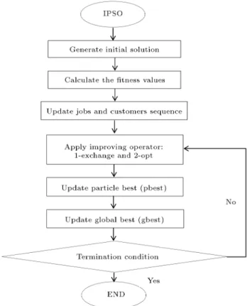
In this section, a particle swarm optimization algorithm named Improved Particle Swarm Optimization (IPSO) algorithm is proposed. The procedure of the IPSO is
Figure 1. Process ow of proposed IPSO.
shown in Figure 1. For this purpose, among many dierent kinds of neighbourhood structures in the literature, a local improvement procedure, namely (1-exchange, 2-opt), is added to improve the solution's quality. It is randomly selected for each iteration to extend solution search. The following two types are considered to improve solution quality and widen search space:
1-exchange: Select two tours; then, omit one customer in one of two tours and add it to the other tour;
2-opt: Select two tours; then, interchange two customers of one tour with two of the other. When a particle is going to stagnate, the improving operators are used to search its neighbourhood to pre-vent premature convergence. The improving structures can inuence quality of the solution. Numerical results show how these procedures prevent the algorithm from getting stuck in a local optimum.
4.2. Computational procedure
The complete computational procedure of the IPSO is summarized as follows:
- Step 1: Initialization:
Initialize P particles randomly as a population with (D = n + c + v 1)-dimensions; n, c, v, respectively refer to the numbers of jobs,
customers, and vehicles. In the production stage, customers are randomly assigned to a denite number of v vehicles. There is a capacity violation cost in order to guarantee the vehicle capacity constraint and time violation cost to satisfy the deadline constraint by minimizing violation costs. In the distribution stage, the permutation of jobs is considered in the initial population with con-sideration of better tness value (lower objective function). First, calculate each particle's tness value of the initialization population and, then, rank them. Choose the smaller one that is Pt
i.
Choose the particle with the best tness value of the whole population as Pt
g;
Set t = 1; generate the position of particle i, X1
i(i = 1; 2; ; p) randomly, where Xi1 =
(x1
i1; x1i2; ; x1iD) for the whole population;
Generate velocity of particle i, V1
i (i = 1; 2; ; p)
randomly, where V1
i = v1i1; v1i2; ; viD1 for the
whole population;
Compute the performance measurement, i.e. the total delivery and tardy cost, and set it as the tness value f1
i of x1i(i = 1; 2; ; p);
For each particle in the swarm, P1
i = (p1i1 =
x1
i1; p1i2= x1i2; ; p1iD= x1iD) for i = 1; 2; ; p;
Find the best tness value in the population P1 g =
min(f1
i) for i = 1; 2; ; p.
- Step 2: Update iteration:
t = t + 1.
- Step 3: Apply improving operator:
Apply one of two improving operators randomly at each iteration to search the solution space widely and achieve various solutions.
- Step 4: Update Pt
i and Pgt:
For i = 1; 2; ; p calculate the tness value; if ft
i < Pit 1, put Pit= fit; otherwise, Pit= Pit 1;
For i = 1; 2; ; p calculate tness value; nd the minimum tness value in the swarm; if min(ft
i) <
Pg(t 1), put Pgt= min(fit); otherwise, Pgt= Pgt 1.
- Step 5: Update velocity:
vt
i = !:vt 1id + c1:r1(ptid xtid) + c2:r2(ptgd xtid);
'1and '2are equal to 2.05; r1and r2are random
numbers uniformly distributed in [0,1], and c1and
c2 are random numbers in [0,2].
- Step 6: Update position
xt
id = xt 1id + vidt.
- Step 7: Termination criterion
The termination criterion is determined when the number of iterations is achieved by the max generation; otherwise, go to Step 2.
Figure 2. The particle encoded as the number of jobs and customers.
4.3. Solution representation in an illustrative example
In an integrated production and distribution scheduling problem, the information of both problems is stored in one particle instead of dening two separate particles. Hence, the encoding scheme contains real numbers. Each particle is consisted to have (n + c + v 1) dimensions, in which n, c, and v are, respectively, the numbers of jobs, customers, and vehicles.
In this section, an illustrative example has been included to show the eciency of the proposed ap-proach. After completion of jobs (Cmax) in the
pro-duction stage, which contains permutation ow shop scheduling, vehicles deliver customers' orders with re-strictions of vehicles capacity and deadline constraint. An instance of the problem with three jobs, eight customers, and three vehicles is given in Figure 2 as an example of the encoding integrated problem. A particle in this encoding system is a feasible sequence of jobs that are assigned to machines in spite of the sequence of customers that are assigned to vehicles with respect to vehicle capacity.
5. Computational results
In this section, the computational experiments are performed to test the performance of the proposed algorithm. The IPSO algorithm is tested on dierent scale instances and compared with the recently pro-posed ecient algorithms. As there are no benchmark solutions to compare with the solution of the proposed algorithm, for small-size and moderate-size instances, the IPSO algorithm is compared with the optimal solution calculated by a commercial optimization soft-ware, LINGO 13.0. For large-size instances, it is compared with the genetic algorithm of the similar problem [4]. All the algorithms in this paper are coded in MATLAB 8.3. They are implemented on a computer with Intel Core 2Duo 2.5 GHZ and 3 GB RAM.
5.1. Test problems generation
Test problems are randomly generated as follows. 25 random instances for each problem size are created based on the following parameter settings:
The job processing time on the machine is randomly generated from the uniform distribution in the range of [1; 99];
The volumes of dierent jobs are randomly gener-ated from the uniform distribution in the range of [1; 10];
The distance between dierent customers is ran-domly generated from the uniform distribution in the range of [1; 100];
The vehicle capacity is randomly generated from the uniform distribution in the range of [Pcj=1 Pn
i=1eij=v, Pcj=1
Pn
i=1eij];
In this paper, a new and practical range is ap-plied with consideration of velocity and distance, the deadlines of which are randomly generated from the uniform distribution in the range of [Pmr=1Pni=1Tri, (Tmin + Tmax)=2 + (dmin +
dmax)=2v], where Tmin and Tmax are minimum and
maximum job processing times, respectively, and dmin and dmax are the minimum and maximum
distances, respectively in which = 0:2 and = 1:5 by numerical experiments. It is dierent from Pundoor and Chen's [13] research;
The due dates are randomly generated from the uniform distribution in range of [du(1 R=2), du(1+ R=2)] that du = Pmr=1Pni=1Tri(1 ), R = 0:6,
= 0:2 [33].
Problems are classied into three groups of small, moderate, and large sizes in order to compare exact procedures, IPSO, and GA, for each test problem that is described in the next section.
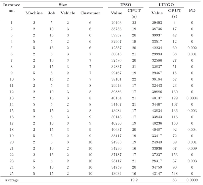
Table 1. Results of random instances with small sizes. Instance
no.
Size IPSO LINGO
PD Machine Job Vehicle Customer Value CPUT
(s) Value
CPUT (s)
1 2 5 2 6 29493 22 29493 4 0
2 2 10 3 6 38736 19 38736 17 0
3 2 15 3 6 39937 20 39937 42 0
4 5 5 2 6 32967 19 33517 12 0
5 5 15 2 6 42337 20 42234 60 0.002
6 2 5 3 7 30043 21 29993 38 0.001
7 2 10 3 7 32586 20 32586 27 0
8 2 15 3 7 32837 21 32837 51 0
9 5 5 2 7 29467 19 29467 15 0
10 5 15 2 7 38101 22 38184 52 0
11 2 5 3 8 29943 17 32443 23 0
12 2 10 3 8 39886 17 39886 160 0
13 2 15 3 8 40154 21 40137 129 0.0004
14 5 5 2 8 34467 21 34467 107 0
15 5 15 2 8 43984 17 43834 136 0.003
16 2 5 3 9 30143 17 33843 116 0
17 2 10 3 9 40236 19 40236 160 0
18 2 15 3 9 40637 20 40487 92 0.004
19 5 5 2 9 33417 19 33417 72 0
20 2 5 3 10 24983 19 24943 59 0.001
21 2 10 2 10 34236 16 33936 67 0.009
22 2 15 2 10 37187 17 37237 153 0
23 5 5 2 10 28417 21 28317 37 0.003
24 5 10 2 10 34759 20 34759 90 0
25 5 15 2 10 43034 16 43147 548 0
Average 19.2 83 0.0009
5.2. Validation and verication of the IPSO In this section, the outcomes of the model in the exact procedure, IPSO, and GA for each test problem, in the way of randomized block design [34], are reported. The tables consist of three parts: the objective function, running time (CPUT), and percentage deviation. The indicator PD (Percentage Deviation) is dened as PD = 100 (IPSOs LINGOs)=LINGOs to assess the quality of the obtained solution. It measures the amount of improvement in terms of the objective function. In the PD formula, LINGOs and IPSOs represent the LINGO solution and IPSO solution, respectively. It should be mentioned that LINGO nds the optimal solution for all small-size instances.
For comparison, the MINLP model is solved with the mathematical software LINGO 13.0. It is used to exactly solve the model with small-size instances. Since the complexity of the problem is categorized in the NP-hard class, only small-size problems can be
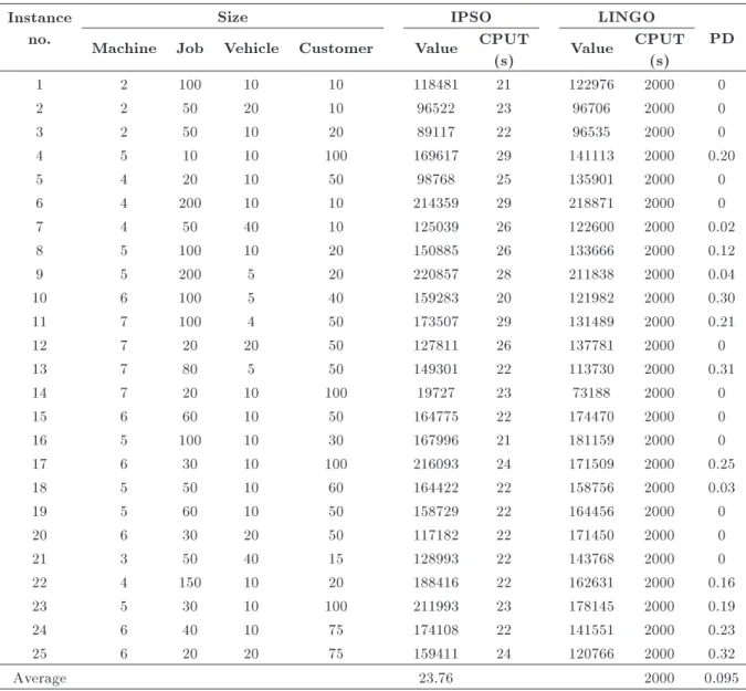
solved. All PD percentages and the total average of the small-size problems shown in Table 1 are less than 0.9%. The average running time of the IPSO is less than that of the optimal approach. For moderate-size problems, LINGO returns a local optimal solution in a limitation of 2000 seconds for running time. Table 2 shows the solutions of the proposed IPSO algorithm, which are better than the local optimal solutions found by LINGO. The gap of the local solution is 9.5% on average for all size instances. For moderate-size problems, the PD formula is rewritten as PD = 100 max(0; IPSOs LINGOs)=LINGOs.
It is shown that the IPSO runs much faster than the LINGO solver. Although the LINGO solver nds the optimal solution, the computational time of LINGO grows exponentially as the instance size increases. Moreover, the IPSO cannot obtain optimal solutions for moderate sizes, but can nd locally optimal solu-tions in the limitation time of 2000 seconds.
Table 2. Results of random instances with moderate sizes. Instance
no.
Size IPSO LINGO
PD Machine Job Vehicle Customer Value CPUT
(s) Value
CPUT (s)
1 2 100 10 10 118481 21 122976 2000 0
2 2 50 20 10 96522 23 96706 2000 0
3 2 50 10 20 89117 22 96535 2000 0
4 5 10 10 100 169617 29 141113 2000 0.20
5 4 20 10 50 98768 25 135901 2000 0
6 4 200 10 10 214359 29 218871 2000 0
7 4 50 40 10 125039 26 122600 2000 0.02
8 5 100 10 20 150885 26 133666 2000 0.12
9 5 200 5 20 220857 28 211838 2000 0.04
10 6 100 5 40 159283 20 121982 2000 0.30
11 7 100 4 50 173507 29 131489 2000 0.21
12 7 20 20 50 127811 26 137781 2000 0
13 7 80 5 50 149301 22 113730 2000 0.31
14 7 20 10 100 19727 23 73188 2000 0
15 6 60 10 50 164775 22 174470 2000 0
16 5 100 10 30 167996 21 181159 2000 0
17 6 30 10 100 216093 24 171509 2000 0.25
18 5 50 10 60 164422 22 158756 2000 0.03
19 5 60 10 50 158729 22 164456 2000 0
20 6 30 20 50 117182 22 171450 2000 0
21 3 50 40 15 128993 22 143768 2000 0
22 4 150 10 20 188416 22 162631 2000 0.16
23 5 30 10 100 211993 23 178145 2000 0.19
24 6 40 10 75 174108 22 141551 2000 0.23
25 6 20 20 75 159411 24 120766 2000 0.32
Average 23.76 2000 0.095
The superiority of the suggested IPSO is ex-amined by analysis of variance and Tukey pairwise comparisons [34]. The statistical model presented in Eq. (4) is the same for both response variables, i.e. objective function and running time. Consequently, Yij can be the objective function or time duration
of the ith test problem solved by the jth algorithm (LINGO, IPSO, or GA). The size of the test problem is considered as the block eect (pi) in I levels and the
algorithm is determined as the main factor (aj) in J
levels. The statistical model is as follows: Yij = + pi+ aj+ "ij;
i = 1; 2; ; I; j = 1; 2; ; J: (23) In order to show that the proposed IPSO converges on the optimal solution in a polynomial time for solving small-size and moderate-size test problems, the results of Tables 1 and 2 are utilized. As mentioned before,
the executions are based on a randomized block design with I = 50 and J = 2.
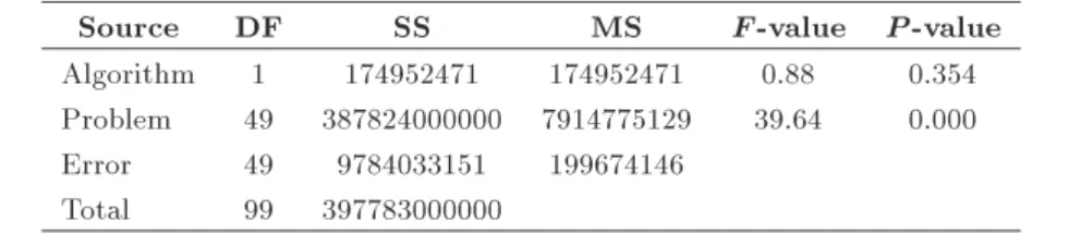
Tables 3 and 4 report the analysis results of variance obtained by a statistical software package, MINITAB 17. Moreover, the results of the Tukey test are reported in Tables 5 and 6. According to Table 3, the equivalence hypothesis of LINGO and IPSO solutions in terms of objective function is not rejected. Furthermore, based on Table 5, both LINGO and IPSO algorithms are categorized in the same group. As a result, the convergence of IPSO on the optimal solution, i.e., the verication of IPSO, is statistically proven.
Tables 4 and 6 represent results of the ANOVA and Tukey test for CPU times, respectively. As the P -value of Table 4 for the algorithm is about zero, LINGO and IPSO solutions are dierent in terms of running times. With dierent categories of the Tukey test in Table 5, it is proven that the running
Table 3. Results of comparing exact solutions and IPSO solutions with respect to objective function.
Source DF SS MS F -value P -value
Algorithm 1 174952471 174952471 0.88 0.354 Problem 49 387824000000 7914775129 39.64 0.000 Error 49 9784033151 199674146
Total 99 397783000000
Table 4. Results of comparing exact solutions and IPSO solutions with respect to running time.
Source DF SS MS F -value P -value
Algorithm 1 26208553 26208553 56.29 0.000 Problem 49 23030099 470002 1.01 0.487 Error 49 22813714 465586
Total 99 72052366 Table 5. Tukey results of comparing exact solutions and IPSO solutions with respect to objective function.
Tukey grouping Mean N Algorithm
A 92947.6 50 LINGO
A 90302.2 50 IPSO
Table 6. Tukey results of comparing exact solutions and IPSO solutions with respect to running time.
Tukey grouping Mean N Algorithm
A 1045.34 50 LINGO
B 21.45 50 IPSO
time of IPSO is much less than that of the LINGO solver.
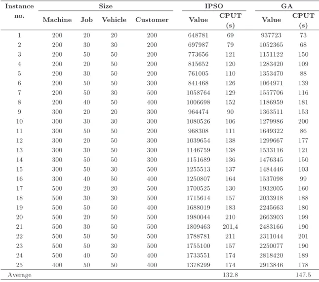
As LINGO cannot solve large-size problems, for these instances, the proposed IPSO algorithm is com-pared with the genetic algorithm proposed by [4] for the similar integrated scheduling problem. This is done to assess the eciency of the proposed algorithm in solving real cases. The PD indicator is not dened here because the optimal solutions are not available. Table 7 presents the results of IPSO and GA in terms of the objective function and the CPU time. The IPSO algorithm is capable of generating solutions with good quality and within a reasonable amount of CPU time, which is less than that in the GA algorithm on average. Using the ANOVA procedure and Tukey test, both IPSO and GA are compared with each other. Results of the statistical model with MINITAB 17, where I = 25 and J = 2, are reported in Tables 8-11. According to Tables 7 and 9, the algorithms are signicantly dierent in terms of the solution's quality. Therefore, IPSO is greatly superior to GA.
In addition to the objective function, the com-parison made between the two algorithms in terms of CPU time is reported in Tables 9 and 11. It shows that running times of both IPSO and GA do not
dier signicantly because the P -value is larger than 5% and they are in the same category of the Tukey test. However, this comparison is not worth mentioning because IPSO and GA are both meta-heuristics which solve problems in polynomial time.
From the above test results, it is found that the proposed IPSO algorithm can solve IPDS eciently, providing reliable solutions. It is more eective and better than the other compared algorithms, i.e. GA and LINGO software. The eciency of the IPSO makes it suitable for solving real cases, which are normally large in scale.
5.3. Managerial implication
This paper discusses the practical implications of man-agerial decisions to integrate production and distribu-tion scheduling. The focus of this study is to show the practical implication of the integrated model to consider simultaneous owshop scheduling and vehicle routing decisions. The integrated scheduling problems studied in this paper are based on the models for production and distribution that are applied to a wide range of practical applications. The integrated ap-proach prevents decrease in product quality, expiration before delivery, extra expenses, and lack of customer satisfaction. It is practical in many industries involving make-to-order or time-sensitive (e.g., perishable, dairy) products, where nished orders are often delivered to customers immediately or shortly after the production to restrict quality reduction.
6. Conclusion and future research
This paper has dealt with practice-oriented integrated production and distribution scheduling. IPDS focuses on products with a short lifespan that include owshop scheduling decisions in a single plant, a eet of limited-capacity trucks for delivering customers' demand with consideration of vehicle routing, and a number of
Table 7. Results of random instances with large sizes. Instance
no.
Size IPSO GA
Machine Job Vehicle Customer Value CPUT
(s) Value
CPUT (s)
1 200 20 20 200 648781 69 937723 73
2 200 30 30 200 697987 79 1052365 68
3 200 50 50 200 773656 121 1151122 150
4 200 20 50 200 815652 120 1283420 109
5 200 30 50 200 761005 110 1353470 88
6 200 50 50 300 841468 126 1064971 139
7 200 50 30 500 1058764 129 1557706 116
8 200 40 50 400 1006698 152 1186959 181
9 300 20 20 300 964474 90 1363511 153
10 300 30 30 300 1080526 106 1279986 200
11 300 50 50 200 968308 111 1649322 86
12 300 20 50 300 1039654 138 1299667 177
13 300 30 50 300 1146759 138 1533116 121
14 300 50 50 300 1151689 136 1476345 150
15 300 50 30 500 1255513 137 1484446 103
16 300 40 50 400 1250807 164 1537098 99
17 500 20 20 500 1700525 130 1932005 160
18 500 30 30 500 1715614 157 2033918 188
19 500 50 50 400 1688019 183 2245663 180
20 500 20 50 500 1980044 210 2663903 199
21 500 30 50 500 1809463 201,4 2483166 190
22 500 50 50 500 1788781 211 2311044 201
23 500 50 30 500 1755100 157 2250077 190
24 500 40 50 400 1733551 174 2818420 189
25 400 50 50 400 1378299 174 2913846 178
Average 132.8 147.5
Table 8. Results of comparing exact solutions and IPSO solutions with respect to the objective function.
Source DF SS MS F -value P -value
Algorithm 1 2809460000000 2809460000000 61.48 0.000 Problem 24 11278000000000 469918000000 10.28 0.000 Error 24 1096650000000 45693786706
Total 49 15184100000000
Table 9. Results of comparing exact solutions and IPSO solutions with respect to the CPU time.
Source DF SS MS F -value P -value
Algorithm 1 545.2 545.2 1.00 0.326 Problem 24 67577.0 2815.7 5.19 0.000 Error 24 13023.5 542.6
Total 49 81145.7
customers with dened locations and demands. The goal was to design routes that serve all customers within each trip and to schedule production in order to minimize the total tardy and delivery costs while fullling the vehicle capacity and deadline for each trip in order to meet lifespan constraints. In the perishable
products industry, costs are perhaps the most promi-nent feature. They are strongly inuenced by the two interrelated stages of production and distribution. In this paper, a scheduling problem in a two-stage sup-ply chain environment is proposed with the objective function of minimizing the sum of delivery and tardy
Table 10. Tukey results of IPSO and GA with respect to the objective function.
Tukey grouping Mean N Algorithm
A 1714531 25 GA
B 1240445 25 IPSO
Table 11. Tukey results of IPSO and GA with respect to the CPU time.
Tukey grouping Mean N Algorithm
A 147.536 25 GA
B 140.932 25 IPSO
costs. The production and distribution scheduling is integrated into ow shop environment and vehicle routing. This model is still a good representation of the real-world cases such as the dairy product industry. After presenting the IPDS problem as a mixed integer nonlinear programming model, since the problem is NP-hard in the strong sense, an Improved Particle Swarm Optimization (IPSO) algorithm was proposed to schedule the integrated problem. 1-exchange and 2-opt improving operators enhanced quality of the solution in IPSO. Since this is the rst study of this problem, a new data set was generated.
Results of the numerical survey indicated de-creasing costs and, as a result, inde-creasing customer satisfaction and product quality. All of the 25 small-size instances were optimally solved by the proposed IPSO. The mean relative deviation from the optimum of 0.9% was close to zero. The gap of the local solution was 9.5% on average for all moderate-size instances. The superiority of the suggested IPSO was examined by analysis of variance and Tukey pairwise comparisons. As a result, the convergence of IPSO on the optimal solution, i.e. the verication of IPSO, was statistically proven. Moreover, for large-size instances, the proposed IPSO algorithm was compared with the genetic algorithm proposed by [4] for the similar integrated scheduling problem. Using the ANOVA procedure and Tukey test, both IPSO and GA were compared. Results of the statistical model reported that the eciency of the IPSO made it suitable for solving real cases, which were normally large in scale. An investigation of large-size instances indicated that the IPSO was able to provide relatively good results within an acceptable computation time.
Future research is needed to investigate an inte-grated scheduling problem where the machine cong-urations and distribution are more complex, such as batch scheduling, two-stage vehicle routing, or multi plants which are distributed in various geographic regions. Integration of dierent decision levels, like tactical or strategic, helps in optimizing the whole supply chain. Tightening the gap between theory and
practical applications would be highly worthwhile for more research.
References
1. Schmid, V., Doerner, K.F. and Laporte, G. \Rich rout-ing problems arisrout-ing in supply chain management", European Journal of Operational Research, 228, pp. 435-448 (2013).
2. Diaz-Madronero, M., Peidro, D. and Mula, J. \A review of tactical optimization models for integrated production and transport routing planning decisions", Computers & Industrial Engineering, 88, pp. 518-535 (2015).
3. Farahani, P., Grunow, M. and Gunther, H.O. \Inte-grated production and distribution planning for per-ishable food products", Flexible Service Manufacturing Journal, 24(1), pp. 28-51 (2012).
4. Ullrich, C.A. \Integrated machine scheduling and ve-hicle routing with time windows", European Journal of Operational Research, 227(1), pp. 152-165 (2013). 5. Chang, Y.C. and Lee, C.Y. \Machine scheduling with
job delivery coordination", European Journal of Oper-ational Research, 158(2), pp. 470-487 (2004).
6. Chen, Z.L. \Integrated production and outbound dis-tribution scheduling: Review and extensions", Opera-tions Research, 58(1), pp. 130-148 (2010).
7. Chen, H.K., Hsueh, C.F. and Chang, M.S. \Production scheduling and vehicle routing with time windows for perishable food products", Computers & Operation Research, 36(7), pp. 2311-2319 (2009).
8. Buer, M.G.V., Woodru, D.L. and Olson, R.T. \Solv-ing the medium newspaper production/distribution problem", European Journal of Operational Research, 115(2), pp. 237-253 (1999).
9. Wang, Q., Batta, R. and Szczerba, R.J. \Sequencing the processing of incoming mail to match an outbound truck delivery schedule", Computers and Operations Research, 32(7), pp. 1777-1791 (2005).
10. Devapriya, P., Ferrell, W. and Geismar, N., Optimal Fleet Size of an Integrated Production and Distribution Scheduling Problem for a Perishable Product, Working Paper, Clemson University (2006).
11. Chandra, P. and Fisher, M.L. \Coordination of pro-duction and distribution planning", European Journal of Operational Research, 72(3), pp. 503-517 (1994). 12. Chen, Z.L. and Vairaktarakis, G.L. \Integrated
scheduling of production and distribution operations", Management Science, 51(4), pp. 614-628 (2005). 13. Pundoor, G. and Chen, Z.L. \Scheduling a
production-distribution system to optimize the tradeo between delivery tardiness and total distribution cost", Naval Research Logistics, 52(6), pp. 571-589 (2005). 14. Chen, Z.L., Handbook of Quantitative Supply Chain
Analysis: Modeling in the EBusiness Era., Kluwer Academic Publishers, Norwell, MA, USA (2004).
15. Lee, C.Y. and Chen, Z.L. \Machine scheduling with transportation considerations", Journal of Scheduling, 4(1), pp. 3-24 (2001).
16. Zhong, W.Y., Dosa, G. and Tan, Z.Y. \On the machine scheduling problem with job delivery coordination", European Journal of Operational Research, 182(3), pp. 1057-1072 (2007).
17. Hajiaghaei Keshteli, M. and Aminnayeri, M. \Solving the integrated scheduling of production and rail trans-portation problem by Keshtel algorithm", 25, pp. 184-203 (2014).
18. Saidi Mehrabad, M., DehnaviArani, S., Evazabadian, F. and Mahmoodian, V. \An ant colony algorithm (ACA) for solving the new integrated model of job shop scheduling and conict-free routing of AGVs", 86, pp. 2-13 (2015).
19. Chen, H.k., Hsue, C.F. and Chang, M.S. \Production scheduling and vehicle routing with time windows for perishable food products", Computers & Operation Research, 36(7), pp. 2311-2319 (2009).
20. Liu, Z., Zhang, Y. and Li, M. \Integrated scheduling of ready-mixed concrete production and delivery", Automation in Construction, 48, pp. 31-43 (2014). 21. Averbakh, I. and Xue, Z. \On-line supply chain
scheduling problems with Preemption", European Journal of Operational Research, 181(1), pp. 500-504 (2007).
22. Zegordi, S.H., Abadi, I.N.K. and BeheshtiNia, M.A. \A novel genetic algorithm for solving production and transportation scheduling in a two-stage supply chain", Computers & Industrial Engineering, 58(3), pp. 373-381 (2007).
23. Cheng, B.Y., Joseph, Y.T. and Li, K. \Integrated scheduling of production and distribution to minimize total cost using an improved ant colony optimization method", Computers & Industrial Engineering, 83, pp. 217-225 (2015).
24. Miller, C.E., Tucker, A.W. and Zemlin, R.A. \Inte-ger programming formulations and traveling salesman problems", Journal of the ACM, 7, pp. 326-329 (1960). 25. Kyparisis, G.J. and Koulamas, C. \Flexible ow shop scheduling with uniform parallel machines", European Journal of Operational Research, 168(3), pp. 985-997 (2006).
26. Pinedo, M.L., Scheduling: Theory, Algorithms, and Systems, Springer Science & Business Media (2012). 27. Garey, M.R. and Johnson, D.S., Computer and
In-tractability, W.H. Freeman and Company, New York (1979).
28. Kulkarni, N.K., Patekar, S., Bhoskar, T. and Kulka-rni, O. \Particle swarm optimization application to mechanical engineering - a review", Material Today: Proceeding, 2(4), pp. 2631-2639 (2015).
29. Guo, Y.W., Li, W.D., Mileham, A.R. and Owen, G.W. \Application of particle swarm optimization in integrated process planning and scheduling", Robotics and Computer-Integrated Manufacturing, 25(2), pp. 28-288 (2009).
30. Kennedy, J. and Eberhart, R.C. \Particle swarm optimization", Paper Presented at the Proceedings of IEEE International Conference on Neural Networks, Australia, pp. 1942-1948 (1995).
31. Banks, A., Vincent, J. and Anyakoha, C. \ A review of particle swarm optimization", Part I: Background and Development, Natural Computing, 6(4), pp. 467-484 (2007).
32. Clerc, M., Particle Swarm Optimization, ISTE Ltd, London (2006).
33. Zegordi, S.H., Itoh, K. and Enkawa, T. \A knowledge-able simulated annealing scheme for the early/tardy ow shop scheduling problem", International Journal of Production Research, 33(5), pp. 1449-1466 (1995). 34. Hicks, C.R., Fundamental Concepts in the Design of
Experiments, 4th Ed., Oxford University Press, New York, (1993).
Biographies
Fateme Marandi is a PhD student in the Department of Industrial Engineering at Amirkabir University, Iran. She received her MSc degree from the Department of Industrial Engineering at Tarbiat Modares University in 2012. Her main areas of research include production planning and scheduling, optimization problems, and meta-heuristics.
Seyed Hesameddin Zegordi is an Associate Pro-fessor of Industrial Engineering in the School of En-gineering at Tarbiat Modares University, Iran. He received his PhD degree from the Department of Industrial Engineering and management at Tokyo In-stitute of Technology, Japan, in 1994. He holds an MSc degree in Industrial Engineering and Systems from Sharif University of Technology, Iran, and a BSc degree in Industrial Engineering from Isfahan University of Technology, Iran. His main areas of teaching and research interests include production planning and scheduling, multi-objective optimization problems, meta-heuristics, quality management, and productivity. He has published several articles in international conferences and academic journals in-cluding European Journal of Operational Research, International Journal of Production Research, Journal of Operational Research Society of Japan, Computers & Industrial Engineering, Amirkabir Journal of Science and Engineering, and Scientia Iranica International Journal of Science and Technology.