Some improved interactive aggregation operators under interval-valued intuitionistic fuzzy environment and its application to decision making process

Sharif University of Technology

Scientia Iranica

Transactions E: Industrial Engineering www.scientiairanica.com

Some improved interactive aggregation operators under

interval-valued intuitionistic fuzzy environment and

their application to decision making process

H. Garg

_{, N. Agarwal}

_{and A. Tripathi}

a. School of Mathematics, Thapar University, Patiala 147004, Punjab, India.

b. Department of Mathematics, Jaypee Institute of Information and Technology, Noida - 201307, U.P., India. Received 22 November 2015; received in revised form 2 January 2016; accepted 16 August 2016

KEYWORDS MCDM; Interval-valued intuitionistic fuzzy set;

Aggregation operator; Hamacher operations.

Abstract.The objective of this manuscript is to present an improved aggregator operator by taking into account the eect of an unknown degree (hesitancy degree) in an Interval-Valued Intuitionistic Fuzzy Sets (IVIFSs) environment. For this, rstly, the shortcomings, of the existing operators are addressed and, then, some improved operational laws on IVIFSs have been introduced. Based on these laws, aggregation operators, namely, an Interval-Valued Intuitionistic Fuzzy Hamacher Interactive Weighted Averaging (IV-IFHIWA), Ordered Weighted Averaging (IVIFHIOWA), and Hybrid Weighted Averaging (IVIFHIHWA), have been proposed. Various properties related to these operators are also investigated. Furthermore, based on these operators, an approach to deal with Multi-Criteria Decision Making (MCDM) problem is developed. Finally, a practical example is provided to illustrate the decision making process.

© 2017 Sharif University of Technology. All rights reserved.

1. Introduction

With the growing complexities of the systems day by day, it is dicult for the decision maker to take a decision within a reasonable time by using uncertain, imprecise and vague information. Intuitionistic Fuzzy Sets (IFS) [1] theory is one of the most permissible theories to handle the uncertainties and impreciseness in the data in comparison to the crisp or probability theory [2-6]. But, in some situations, it is dicult to give the preference of an object in terms of a point value and, therefore, it is convenient to express the decision makers information/preferences in the form of interval values, hence called Interval-Valued Intu-itionistic Fuzzy Sets (IVIFSs) [7]. Nowadays, decision

*. Corresponding author.

E-mail address: [email protected] (H. Garg) doi: 10.24200/sci.2017.4386

making is one of the most signicant and omnipresent human activities in business, service, manufacturing, selection of products, etc. It is understandable that the dierent criteria in the decision problem are likely to play dierent roles in reaching a nal decision; thus, the primary objective in the phase of decision making is the information aggregation process. For this, Yager [8] proposed the Ordered Weighted Average (OWA) operator by giving some weights to all the inputs according to their ranking positions. Based on this pioneering work, many extensions have appeared. As IVIFSs are much easier to handle the fuzzy decision information up to the desired degree of accuracy, some researchers have applied the interval-valued intuition-istic fuzzy set theory to the eld of decision making. For instance, Xu and Chen [9], and Xu [10] developed some arithmetic and geometric aggregation operators, namely, interval-valued intuitionistic fuzzy weighted averaging operator and geometric operator, respec-tively, for aggregating the interval-valued intuitionistic

fuzzy information. Furthermore, Xu and Chen [11], and Wei and Wang [12], respectively, developed ordered weighted and hybrid weighted geometric aggregator operators in the interval-valued intuitionistic fuzzy environment. Wang and Liu [13,14] investigated these aggregation operators by using Einstein operations. Later on, Wang and Liu [15,16] extended these op-erators from IFSs to the IVIFSs environments. Wei and Zhao [17] proposed induced hesitant and Zhao et al. [18] developed some hesitant triangular aggregation operators under interval-valued Einstein operations. Apart from that, various researchers have paid more attention to decision-making process for aggregating the dierent alternatives using dierent aggregation operators [19-34] and their corresponding references.

Almost all the above studies are reliable under the restriction that the grade of membership or non-membership of Interval-Valued Intuitionistic Fuzzy Numbers (IVIFNs) is non-zero. For instance, consider two IFSs or IVIFSs, A and B, such that either A= 0 and B 6= 0 or A = 0 and B 6= 0; then, based on an aggregated operator proposed by Xu [3], Wang and Liu [13,15], Zhao [18], Zhang [23] and Liu [25]. The overall aggregated grade of either membership or non-membership values is zero, respectively, for geometric or an averaging aggregated operator. In other words, we can say that the eects of the other grades of either membership or non-membership on a corresponding geometric or an averaging aggregator operator do not play any signicant role during the aggregation process. Furthermore, it has been concluded from the above aggregation process that the grades of overall membership (non-membership) functions are indepen-dent of their corresponding grades of non-membership (membership) functions. Thus, changing any values in the grades does not aect the overall aggregation process. Therefore, the corresponding results are undesirable and get an unreasonable preference order of the alternatives. Hence, there is a need to modify the existing operations by properly considering the degrees of membership functions.

Thus, the objective of this manuscript is to present some series of averaging aggregation operators in an IVIFSs environment. For it, a new operational law on dierent IVIFNs has been proposed by taking the interaction between the pair of membership and non-membership functions. Based on these new op-erational laws, weighted aggregated operators, namely Interval-Valued Intuitionistic Fuzzy (IVIF) Hamacher Interactive Weighted Aggregation (IVIFHIWA), IVIF Hamacher Interactive Ordered Weighted Aggregation (IVIFHIOWA), and IVIF Hamacher Interactive Hy-brid Weighted Aggregation (IVIFHIHWA), have been proposed by properly handling the shortcoming of the existing operators. The main signicance of these operators is that the inuence of the degree of

non-membership function is less than that of the member-ship functions and, hence, these operators, are more optimistic than the others existing in the literature, especially when one of the non-membership degrees is zero. Furthermore, these operators have been tested on the problem of MCDM, where the most desirable alternative is computed under the set of dierent criteria. Finally, the computed results are compared with the results of the existing operators for showing the optimistic nature of the operation.

The rest of the manuscript is organized as follows. In Section 2, some basic denitions related to IVIFSs and their corresponding aggregation operators are sum-marized along with their shortcomings. In Section 3, some new operational laws are dened and, then, we develop some averaging aggregation operators, namely, IVIFHIWA, IVIFHIOWA, and IVIFHIHWA. Desirable properties corresponding to these operators, such as idempotency, boundedness, commutativity, homogene-ity, etc., are also discussed in this section. In section 4, a method based on the proposed operators for solving MCDM problems, where individual assessment is pro-vided as IVIFNs, is presented. An illustrative example has been provided related to MCDM problem, and comparison of the results with the existing methods is given in Section 5. Finally, some concrete conclusion of the paper has been summarized in section 6. 2. Preliminaries

2.1. Intuitionistic and interval-valued intuitionistic fuzzy sets

An Intuitionistic Fuzzy Set (IFS) A [1] in a nite universe of discourse X = fx1; x2; : : : ; xng is given by:

A = fhx; A(x); A(x)i j x 2 Xg;

where A(x) and A(x) are respectively the grades of membership and non-membership of an element x with the conditions that 0 A(x); A(x) 1 and A(x) + A(x) 1, while an interval-valued intuitionistic fuzzy set (IVIFSs) is dened as [7]:

A = fhx; [L

A(x); UA(x)]; [LA(x); AU(x)]i j x 2 Xg; where U

A(x) + AU(x) 1; 0 LA(x) UA(x) 1; 0 L

A(x) AU(x) 1. Clearly, for every x 2 X, if: A(x) = LA(x) = UA(x); A(x) = AL(x) = AU(x); then, IVIFS is reduced to an IFS.

In order to compare the two Interval-Valued Intuitionistic Fuzzy Numbers (IVIFNs), Xu [3] dened the score and accuracy function as S() = a+b c d

2 and H() = a+b+c+d

2 , respectively, for an IVIFN = h[a; b]; [c; d]i. Later on, Wang et al. [35] introduced two new functions called the membership uncertainty

index, G() = b + d a c, and the hesitation uncertainty index, T () = b + c a d, for comparing the two distinct IVIFNs. Based on these functions, a prioritized comparison method for any two IVIFNs = h[a1; b1]; [c1; d1]i and = h[a2; b2]; [c2; d2]i is dened as:

1. If S() > S() then ;

2. If S() < S() then ;

3. If S() = S() then:

i. If H() > H() then ;

ii. If H() < H() then ;

iii. If H() = H(), then:

a. If T () > T (), then ;

b. If T () < T (), then ;

c. If T () = T (), then:

ˆ If G() > G(), then ;

ˆ If G() < G(), then ;

ˆ If G() = G(), then = . 2.2. Hamacher t-norm and t-conorm

T-norm (t) and t-cornorm (T ) are used to dene the union and intersection of two IFSs (IVIFSs), A and B, as follows:

A \ B =fhx; t(A(x); B(x)); T (A(x); B(x))i j x 2 Xg;

A [ B =fhx; T (A(x); B(x)); t(A(x); B(x))i j x 2 Xg:

Hamacher [36] proposed a more generalized t-norm and t-cot-norm by dening:

t(x; y) = _{+ (1 )(x + y xy)}xy ; and:

T (x; y) = x + y xy (1 )xy_{1 (1 )xy} ;

respectively. It is clearly seen from these norms that when = 1, the equations are reduced to algebraic t-norm and t-cornorm, t(x; y) = xy and T (x; y) = x + y xy. Similarly, when = 2, they are respectively reduced to Einstein t-norm and t-cornorm as t(x; y) = _{1+(1 x)(1 y)}xy and T (x; y) = _1+xyx+y. Based on these norms, dierent aggregation operators have been proposed by Liu [25] for aggregating the dierent IVIFNs, i = h[ai; bi]; [ci; di]i; (i = 1; 2; : : : ; n), by using weight vector, ! = (!1; !2; : : : ; !n)T, of i such that !i> 0 and

n P

i=1!i= 1 as:

The Interval-Valued Intuitionistic Fuzzy Hamacher

Weighted Averaging (IVIFHWA) operator is calculated as follows:

IVIFHWA(1; 2; : : : ; n)=!11!22: : : !nn

=

Qn

i=1(1 + ( 1)ai) !i Qn

i=1(1 ai) !i

n Q

i=1(1 + ( 1)ai)

!i+ ( 1)Qn

i=1(1 ai) !i

;

n Q

i=1(1 + ( 1)bi) !i Qn

i=1(1 bi) !i

n Q

i=1(1 + ( 1)bi)

!i+ ( 1)Qn

i=1(1 bi) !i

Qn

i=1c !i

i n

Q

i=1(1 + ( 1)(1 ci))

!i+ ( 1)

n Q i=1c

!i

i ;

Qn i=1d

!i

i n

Q

i=1(1 + ( 1)(1 di))

!i+ ( 1)

n Q i=1d

!i

i

:

The Interval-Valued Intuitionistic Fuzzy Hamacher Or-dered Weighted Averaging (IVIFHOWA) operator is calculated as follows:

IVIFHOWA(1; 2; : : : ; n)

= !1(1) !2(2) : : : !n(n)

=

Qn

i=1(1 + ( 1)a(i)) !i Qn

i=1(1 a(i)) !i

n Q

i=1(1 + ( 1)a(i))

!i+ ( 1)

n Q

i=1(1 a(i)) !i

;

n Q

i=1(1 + ( 1)b(i)) !i Qn

i=1(1 b(i)) !i

n Q

i=1(1 + ( 1)b(i))

!i+ ( 1)Qn

i=1(1 b(i)) !i

Qn

i=1c !i

(i) n

Q

i=1(1 + ( 1)(1 c(i)))

!i+ ( 1)Qn

i=1c !i

(i) ;

Qn i=1d

!i

(i) n

Q

i=1(1 + ( 1)(1 d(i)))

!i+ ( 1)Qn

i=1d !i

(i)

;

where ((1); (2); : : : ; (n)) is a permutation of (1; 2; : : : ; n) such that (i 1) (i) for all i = 1; 2; : : : ; n.

The Interval-Valued Intuitionistic Fuzzy Hamacher Hybrid Weighted Averaging (IVIFHHWA) operator is calculated as follows:

IVIFHHWA(1; 2; : : : ; n)

= !1_(1) !2_(2) : : : !n_(n)

=

Qn

i=1(1+( 1)_a(i)) !i Qn

i=1(1 _a(i)) !i

n Q

i=1(1 + ( 1)_a(i))

!i+( 1)Qn

i=1(1 _a(i)) !i

;

n Q

i=1(1 + ( 1)_b(i)) !i Qn

i=1(1 _b(i)) !i

n Q

i=1(1 + ( 1)_b(i))

!i+ ( 1)

n Q

i=1(1 _b(i)) !i

Qn

i=1_c !i

(i) n

Q

i=1(1 + ( 1)(1 _c(i)))

!i+ ( 1)Qn

i=1_c !i

(i) ;

Qn i=1 _d

!i

(i) n

Q

i=1(1 + ( 1)(1 _d(i)))

!i+ ( 1)Qn

i=1 _d !i

(i)

;

where _(i) is the ith largest weighted intuitionistic fuzzy value _i ( _i= nwii; i = 1; 2; : : : ; n).

2.3. Shortcomings of the existing work

The following shortcomings have been observed in the operators, which prevent the existing operators from giving the sucient information in the phase of the aggregation process.

Example 2.1.

Let 1 = h[0:23; 0:33]; [0; 0]i, 2 = h[0:65; 0:72]; [0:22; 0:27]i, 3 = h[0:31; 0:35], [0:55; 0:58]i, and 4= h[0:17; 0:23]; [0:65; 0:69]i be four IVIFNs and ! = (0:2; 0:3; 0:4; 0:1)T _{be the standardized weight vector} of these numbers; then, by using IVIFHWA operator, to aggregate these IVIFNs, we get the aggregated IVIFN as h[0:4139; 0:4834]; [0; 0]i corresponding to = 1 and h[0:4010; 0:4703]; [0; 0]i corresponding to = 2. From these results, it is seen that the degree of non-membership is zero and is independent of the parameter . Furthermore, this degree is independent of the degree of the other non-memberships (those which are nonzero in i's), which hence play an insignicant role during the aggregation process. Example 2.2.

Let 1 = h[0:23; 0:33]; [0:35; 0:45]i, 2 = h[0:45; 0:55];

[0:23; 0:28]i, 3 = h[0:65; 0:73], [0:17; 0:21]i and 4 = h[0:50; 0:60]; [0:20; 0:30]i be four IVIFNs and ! = (0:2; 0:3; 0:4, 0:1)T _{be the standardized weight vector} of these numbers. Then, based on IVIFHWA operator we get the aggregated IVIFNs as h[0:5137; 0:6074], [0:2186; 0:2763]i by taking = 1 and h[0:5060; 0:6011], [0:2196; 0:2783]i when = 2. On the other hand, if we replace the IVIFNs 2and 3 with:

2= h[0:32; 0:36]; [0:23; 0:28]i; and:

3= h[0:37; 0:40]; [0:17; 0:21]i;

then their corresponding aggregated IVIFNs become h[0:3443; 0:3995], [0:2186; 0:2763]i when = 1 and h[0:3422; 0:3973], [0:2196; 0:2783]i when = 2. Hence, it is seen that the degree of non-membership values of aggregator IVIFN becomes independent of the change of the degree of membership values. Therefore, it is inconsistent and, hence, does not give correct informa-tion to the decision maker.

Therefore, the existing operators, as proposed by Liu [25], are invalid to rank the alternative and, hence, there is a necessity to pay more attention to these issues.

3. Improved operational laws for intuitionistic fuzzy Hamacher aggregation operators Here, we dene some new operational laws for IVIFNs, which overcome the shortcomings of the existing oper-ators as follows.

Denition 3.1.

Let = h[a; b]; [c; d]i and i = h[ai; bi]; [ci; di]i (i = 1; 2) be a collection of the IVIFNs and > 0 be a real number; then, the new operational rules for these IVIFNs are dened as follows:

(i):

1 2=

* Q2

i=1

1 + ( 1)ai 2 Q

i=1(1 ai) 2

Q i=1

1 + ( 1)ai+ ( 1) 2 Q

i=1(1 ai) ;

2 Q i=1

1 + ( 1)bi 2 Q

i=1(1 bi) 2

Q i=1

1 + ( 1)bi+ ( 1) 2 Q

i=1(1 bi)

;

Q2

i=1(1 ai) 2 Q i=1

1 ai ci 2

Q i=1

1 + ( 1)ai+ ( 1) 2 Q

i=1(1 ai) ;

Q2

i=1(1 bi) 2 Q i=1

1 bi di 2

Q i=1

1 + ( 1)bi+ ( 1) 2 Q

i=1(1 bi) +

:

(ii):

1 2=

* Q2

i=1(1 ai) 2 Q i=1

1 ai ci 2

Q i=1

1 + ( 1)ai+ ( 1) 2 Q

i=1(1 ai) ;

Q2

i=1(1 bi) 2 Q i=1

1 bi di 2

Q i=1

1 + ( 1)bi+ ( 1) 2 Q

i=1(1 bi)

;

Q2

i=1

1 + ( 1)ai 2 Q

i=1(1 ai) 2

Q i=1

1 + ( 1)ai+ ( 1) 2 Q

i=1(1 ai) ;

2 Q i=1

1 + ( 1)bi 2 Q

i=1(1 bi) 2

Q i=1

1 + ( 1)bi+ ( 1) 2 Q

i=1(1 bi) +

:

(iii):

=

*

1 + ( 1)a 1 a

1 + ( 1)a+ ( 1)1 a;

1 + ( 1)b 1 b

1 + ( 1)b+ ( 1)1 b

;

_{1 a 1 a c}

1 + ( 1)a+ ( 1)1 a; 1 b 1 b d

1 + ( 1)b+ ( 1)1 b +

:

(iv):

₌*

1 a 1 a c

1 + ( 1)a+ ( 1)1 a; 1 b 1 b d

1 + ( 1)b+ ( 1)1 b

1 + ( 1)a 1 a

1 + ( 1)a+ ( 1)1 a;

1 + ( 1)b 1 b

1 + ( 1)b+ ( 1)1 b +

:

As it is clearly observed from the above denition, the sum of IVIFNs becomes more optimistic than the existing sum because the non-membership degree of 1 2 contains the pairs of membership and non-membership, i.e., ai ci and bi di, while member-ship function does not. Hence, the attitude is more inclined towards the membership function than the non-membership one; therefore, the decision is more optimistic. Now, based on these operations, averaging aggregation operators have been proposed as follows. 3.1. Interval-valued Intuitionistic fuzzy

Hamacher Interactive Weighting Averaging operator

Denition 3.2.

Let i; (i = 1; 2; : : : ; n) be the collection of IVIFNs, and IVIFHIWA : n _{! , if:}

IVIFHIWA(1; 2; : : : ; n)=!11!22: : :!nn; where is the set of IVIFNs and ! = (!1; !2; : : : ; !n)T is the weight vector of i with !i > 0 and

n P i=1!i = 1; therefore, IVIFHIWA is called an interval valued intuitionistic fuzzy Hamacher interactive weighting av-eraging operator.

Theorem 3.1.

Let i = h[ai; bi]; [ci; di]i; (i = 1; 2; : : : ; n) be the collection of IVIFNs, then:

IVIFHIWA(1; 2; : : : ; n)

=

* Qn

i=1(1 + ( 1)ai) !i Qn

i=1(1 ai) !i

n Q

i=1(1 + ( 1)ai)

!i+ ( 1)

n Q

i=1(1 ai) !i

;

n Q

i=1(1 + ( 1)bi) !i Qn

i=1(1 bi) !i

n Q

i=1(1 + ( 1)bi)

!i+ ( 1)Qn

i=1(1 bi) !i

_Qn

i=1(1 ai) !i Qn

i=1(1 ai ci) !i

n Q

i=1(1 + ( 1)ai)

!i+ ( 1)

n Q

i=1(1 ai) !i

;

_Qn

i=1(1 bi) !i Qn

i=1(1 bi di) !i

n Q

i=1(1+( 1)bi)

!i+( 1)Qn

i=1(1 bi) !i

+ : (1)

Proof

When n = 1 and !1= 1, we have:

IVIFHIWA(1) = !11= h[a1; b1]; [c1; d1]i

=

* _{(1 + ( 1)a}

1)1 (1 a1)1 (1 + ( 1)a1)1+ ( 1)(1 a1)1;

(1 + ( 1)b1)1 (1 b1)1 (1 + ( 1)b1)1+ ( 1)(1 b1)1

;

(1 a1)1 (1 a1 c1)1 (1 + ( 1)a1)1+ ( 1)(1 a1)1;

(1 b1)1 (1 b1 d1)1 (1 + ( 1)b1)1+ ( 1)(1 b1)1

+ :

Thus, Eq. (1) holds for n = 1. Assume that Eq. (1) holds for n = k, i.e.:

IVIFHIWA(1; 2; : : : ; k)

=

Qk

i=1(1 + ( 1)ai) !i Qk

i=1(1 ai) !i

k Q

i=1(1 + ( 1)ai)

!i+ ( 1)Qk

i=1(1 ai) !i

;

k Q

i=1(1 + ( 1)bi) !i Qk

i=1(1 bi) !i

k Q

i=1(1 + ( 1)bi)

!i+ ( 1)Qk

i=1(1 bi) !i

_Qk

i=1(1 ai) !i Qk

i=1(1 ai ci) !i

k Q

i=1(1 + ( 1)ai)

!i+ ( 1)Qk

i=1(1 ai) !i

;

_Qk

i=1(1 bi) !i Qk

i=1(1 bi di) !i

k Q

i=1(1 + ( 1)bi)

!i+ ( 1)Qk

i=1(1 bi) !i

:

Then, when n = k + 1, we have:

IVIFHIWA(1; 2; : : : ; k+1) = k+1 M i=1

!ii

= IVIFHIWA(1; 2; : : : ; k) !k+1k+1

=

Qk

i=1(1 + ( 1)ai) !i Qk

i=1(1 ai) !i

k Q

i=1(1 + ( 1)ai)

!i+ ( 1)Qk

i=1(1 ai) !i

;

k Q

i=1(1 + ( 1)bi) !i Qk

i=1(1 bi) !i

k Q

i=1(1 + ( 1)bi)

!i+ ( 1)Qk

i=1(1 bi) !i

;

_Qk

i=1(1 ai) !i Qk

i=1(1 ai ci) !i

k Q

i=1(1 + ( 1)ai)

!i+ ( 1)Qk

i=1(1 ai) !i

;

_Qk

i=1(1 bi) !i Qk

i=1(1 bi di) !i

k Q

i=1(1+( 1)bi)

!i+( 1) Qk

i=1(1 bi) !i

* _{(1+( 1)a}

k+1)wk+1 (1 ak+1)wk+1 (1+( 1)ak+1)wk+1+( 1)(1 a_k+1)wk+1;

(1+( 1)bk+1)wk+1 (1 bk+1)wk+1 (1+( 1)bk+1)wk+1+( 1)(1 b_k+1)wk+1

;

(1 ak+1)wk+1 (1 ak+1 ck+1)wk+1 (1+( 1)ak+1)wk+1+ ( 1)(1 a_k+1)wk+1;

(1 bk+1)wk+1 (1 bk+1 dk+1)wk+1 (1+( 1)bk+1)wk+1+( 1)(1 b_k+1)wk+1

+

=

k+1Q

i=1(1 + ( 1)ai)

!i k+1Q

i=1(1 ai) !i

k+1_Q

i=1(1 + ( 1)ai)

!i+ ( 1)k+1Q

i=1(1 ai) !i

;

k+1_Q

i=1(1 + ( 1)bi)

!i k+1Q

i=1(1 bi) !i

k+1_Q

i=1(1 + ( 1)bi)

!i+ ( 1)

k+1_Q i=1(1 bi)

!i

:

Thus results are true for n = k + 1; hence, by the principle of mathematical induction, results are true for all n 2 Z+_.

Example 3.1

If we apply the proposed IVIFHIWA operator to aggregate the dierent IVIFNs as given in Ex-ample 2.1, then we get aggregated IVIFNs, as h[0:4139; 0:4834]; [0:3886; 0:4545]i when = 1 and h[0:4010; 0:4703], [0:3972; 0:4660]i when = 2. From this, it is seen that the degree of non-membership function is non-zero; even non-membership function of one of the IVIFNs is zero. Thus, non-membership function of IVIFNs plays a dominant role during the aggregation process by the proposed operator.

Example 3.2

If we apply the proposed IVIFHIWA operator to aggregate the dierent IVIFNs as given in Example 2.2, then we get aggregated IVIFN, h[0:5137; 0:6074], [0:2196; 0:2807]i when = 1 and h[0:5060; 0:6011], [0:2231; 0:2852]i when = 2. On the other hand, if we apply the proposed aggregated operator to modi-ed IVIFNs then we get IVIFHIWA(1; 2; 3; 4) = h[0:3443; 0:3995], [0:2257; 0:3042]i for = 1 and h[0:3422; 0:3973], [0:2264; 0:3053]i for = 2. Thus, the change of membership function will aect the degree of non-membership functions and is non-zero. Therefore, there is a proper interaction between the degrees of membership and non-membership functions and, hence, the results are consistent and more practical than the results of the existing operators.

Lemma 3.1 [3]

Let i, !i> 0 for i = 1; 2; : : : ; n and n P

i=1!i= 1, then: n

Y i=1

!i

i

n X i=1

!ii;

which equality holds if and only if 1= 2= : : : = n. Corollary 3.1

The IVIFHWA and IVIFHIWA operators have the following relation:

IVIFHIWA(1; 2; : : : ; n) IVIFHWA(1; 2; : : : ; n);

where i (i = 1; 2; : : : ; n) is a collection of IVIFNs. ! = (!1; !2; : : : ; !n)T is the weight vector of i such that !i> 0, i = 1; 2; : : : ; n and

n P i=1!i= 1 Proof

Let IVIFHIWA(1; 2; : : : ; n) = h[ap; bp]; [cp; dp]i

= p _{and IVIFHWA(}

1; 2; : : : ; n) = h[a; b]; [c; d]i = . Since:

n Y i=1

(1 + ( 1)ai)!i+ ( 1) n Y i=1

(1 ai)!i

Xn i=1

!i(1 + ( 1)ai)

+ ( 1)Xn i=1

!i(1 ai) = ;

fQn

i=1(1 ai) !i Qn

i=1(1 ai ci) !ig

n Q

i=1(1 + ( 1)ai)

!i+ ( 1)

n Q

i=1(1 ai) !i

n Y i=1

(1 ai)!i n Y i=1

(1 ai ci)!i

Qn i=1c

!i

i n

Q

i=1(1 + ( 1)(1 ci))

!i+ ( 1)Qn

i=1c !i

i :

Thus ap

= aand cp c, where equality holds if and only if a1 = a2 = : : : = an and c1 = c2 = : : : = cn. Similarly, bp

= band dp d. Thus: S(p_{) =} ap+ bp cp dp

2

a+ b c d 2

= S():

If S(p_{) < S(), then for every !, we have:} IVIFHIWA(1; 2; : : : ; n)

< IVIFHWA(1; 2; : : : ; n): If S(p_{) = S(), i.e.:} ap

+bp cp dp

2 = a+b2c d then, by the condition cp

c and dp d, we have ap

= a, bp = b, cp = c and dp = d; thus, the accuracy function is: H(p_{) =} ap

+bp+cp+dp

2 =

a+b+c+d

2 = H(): Therefore, in this case, from the denition of score function, it follows that:

IVIFHIWA(1; 2; : : : ; n)

= IVIFHWA(1; 2; : : : ; n): Hence:

IVIFHIWA(1; 2; : : : ; n)

IVIFHWA(1; 2; : : : ; n);

where that equality holds if and only if 1 = 2 = : : : = n.

Therefore, it has been concluded from Corollary 3.1 that the proposed IVIFHIWA operator shows the decision maker's attitude more optimistically than the existing IVIFHWA operator [25] during the aggrega-tion process.

Theorem 3.2

If i= h[ai; bi]; [ci; di]i, (i = 1; 2; : : : ; n) be a collection of IVIFNs, then the aggregated value by IVIFHIWA operator is also an IVIFN; i.e.:

Proof

Since i = h[ai; bi]; [ci; di]i is an IVIFN, for i = 1; 2; : : : ; n, by denition of IVIFN, we have:

0 ai; bi; ci; di 1 and bi+ di 1 IVIFHIWA(1; : : : ; n) = h[ap; bp]; [cp; dp]i as:

n Q

i=1(1 + ( 1)ai) !i Qn

i=1(1 ai) !i

n Q

i=1(1 + ( 1)ai)

!i+ ( 1)(1 a_i)!i

= 1

Qn

i=1(1 ai) !i

n Q

i=1(1 + ( 1)ai)

!i+ ( 1)Qn

i=1(1 ai) !i

1 Yn i=1

(1 ai)!i 1: Also:

1 + ( 1)ai (1 ai)

, n Y i=1

(1 + ( 1)ai)!i n Y i=1

(1 ai)!i 0

, n Q

i=1(1 + ( 1)ai) !i Qn

i=1(1 ai) !i

n Q

i=1(1 + ( 1)ai)

!i+ ( 1)Qn

i=1(1 ai) !i

0:

Thus, 0 ap

1. On the other hand: Qn

i=1(1 ai) !i Qn

i=1(1 ai ci) !i

n Q

i=1(1 + ( 1)ai)

!i+ ( 1)

n Q

i=1(1 ai) !i

Qn

i=1(1 ai) !i

n Q

i=1(1 + ( 1)ai)

!i+ ( 1)Qn

i=1(1 ai) !i

Yn i=1

(1 ai)!i 1: Also:

n Y i=1

(1 ai)!i n Y i=1

(1 ai ci)!i 0

,

Qn

i=1(1 ai) !i Qn

i=1(1 ai ci) !i

n Q

i=1(1 + ( 1)ai)

!i+ ( 1)Qn

i=1(1 ai) !i

0:

Thus 0 cp

1. Moreover: ap

+ cp= 1

Qn

i=1(1 ai ci) !i

n Q

i=1(1 + ( 1)ai)

!i+ ( 1)

n Q

i=1(1 ai) !i

1 n Y i=1

(1 ai ci)!i 1:

Similarly, 0 bp

1, 0 dp 1 and bp+ dp 1. Hence, IVIFHIWA 2 [0; 1]. Therefore, the aggre-gated IVIFN is again an IVIFN.

Based on Theorem 3.1, we have some properties of the proposed IVIFHIWA operator for a collection of IVIFNs i = h[ai; bi]; [ci; di]i(i = 1; 2; : : : ; n), and ! = (!1; !2; : : : ; !n)T is the associated weighted vector satisfying !i> 0 and

n P i=1!i= 1. Property 3.1 (Idempotency)

If i= 0= h[a0; b0]; [c0; d0]i for all i, then: IVIFHIWA(1; 2; : : : ; n) = 0:

Proof

Since i = 0 = h[a0; b0]; [c0; d0]i(i = 1; 2; : : : ; n), and n

P

i=1!i= 1, by Theorem 3.1, we have: IVIFHIWA(1; 2; : : : ; n)

=

* Qn

i=1(1 + ( 1)a0) !i Qn

i=1(1 a0) !i

n Q

i=1(1 + ( 1)a0)

!i+ ( 1)

n Q

i=1(1 a0) !i

;

n Q

i=1(1 + ( 1)b0) !i Qn

i=1(1 b0) !i

n Q

i=1(1 + ( 1)b0)

!i+ ( 1)Qn

i=1(1 b0) !i

;

_Qn

i=1(1 a0) !i Qn

i=1(1 a0 c0) !i

n Q

i=1(1 + ( 1)a0)

!i+ ( 1)

n Q

i=1(1 a0) !i

;

_Qn

i=1(1 b0) !i Qn

i=1(1 b0 d0) !i

n Q

i=1(1 + ( 1)b0)

!i+ ( 1)Qn

i=1(1 b0) !i

=

* _{(1 + ( 1)a}

0)

n

P

i=1!i (1 a₀) n

P

i=1!i

(1 + ( 1)a0)

n

P

i=1!i+ ( 1)(1 a₀) n

P

i=1!i

;

(1 + ( 1)b0)

n

P

i=1!i (1 b₀) n

P

i=1!i

(1 + ( 1)b0)

n

P

i=1!i+ ( 1)(1 b₀) n

P

i=1!i

;

(1 a0)

n

P

i=1!i (1 a₀ c₀) n

P

i=1!i

(1 + ( 1)a0)

n

P

i=1!i+ ( 1)(1 a₀) n

P

i=1!i

;

(1 b0)

n

P

i=1!i (1 b₀ d₀) n

P

i=1!i

(1 + ( 1)b0)

n

P

i=1!i+ ( 1)(1 b₀) n

P

i=1!i

+

=

* _{(1 + ( 1)a}

0) (1 a0) (1 + ( 1)a0) + ( 1)(1 a0);

(1 + ( 1)b0) (1 b0) (1 + ( 1)b0) + ( 1)(1 b0)

;

(1 a0) (1 a0 c0)

(1 + ( 1)a0) + ( 1)(1 a0);

(1 b0) (1 b0 d0)

(1 + ( 1)b0) + ( 1)(1 b0) +

= h[a0; b0]; [c0; d0]i = 0:

Property 3.2 (Boundedness)

Let = min(1; 2; : : : ; n), + = max(1; 2; : : : ; n), then:

IVIFHIWA(1; 2; : : : ; n) +: Proof

Let f(x) = 1 x

1+( 1)x; x 2 [0; 1] then f

0

(x) =

(1+( 1)x)2 < 0; thus, f(x) is decreasing

func-tion. Since ai;min ai ai;max, for all i = 1; 2; : : : ; n, f(ai;max) f(ai) f(ai;min) for all i, i.e.,

1 ai;max

1+( 1)ai;max

1 ai

1+( 1)ai

1 ai;min

1+( 1)ai;min for all i.

Let ! = (!1; !2; : : : ; !n)T be the associated weighted vector satisfying !i > 0 and

n P

i=1!i = 1; then, for all i, we have:

1 ai;max 1 + ( 1)ai;max

_!i

1 ai 1 + ( 1)ai

_!i

1 ai;min 1 + ( 1)ai;min

!i : Thus: n Y i=1

1 ai;max 1 + ( 1)ai;max

_!i Yn

i=1

1 ai 1 + ( 1)ai

_!i

Yn i=1

1 ai;min 1 + ( 1)ai;min

!i

, ( 1)

1 ai;max 1 + ( 1)ai;max

( 1) n Y i=1

1 ai 1 + ( 1)ai

!i

( 1)

1 ai;min 1 + ( 1)ai;min

,

1 + ( 1)ai;max

1 + ( 1) n Y i=1

1 ai 1 + ( 1)ai

!i

1 + ( 1)ai;min

,

1 + ( 1)ai;min

1

1 + ( 1)Qn i=1

1 ai 1 + ( 1)ai

_!i

1 + ( 1)ai;max

, 1 + ( 1)ai;min

1 + ( 1)Qn i=1

1 ai 1 + ( 1)ai

!i

1 + ( 1)ai;max , ( 1)ai;min

1 + ( 1)Qn i=1

1 ai 1 + ( 1)ai

( 1)ai;max , ai;min

n Q

i=1(1 + ( 1)ai) !i Qn

i=1(1 ai) !i

n Q

i=1(1 + ( 1)ai)

!i+ ( 1)Qn

i=1(1 ai) !i

ai;max: (2)

Similarly:

bi;min n Q

i=1(1 + ( 1)bi) !i Qn

i=1(1 bi) !i

n Q

i=1(1 + ( 1)bi)

!i+ ( 1)Qn

i=1(1 bi) !i

bi;max: (3)

On the other hand, let g(y) = ( 1)y_{( 1)y} ; y 2 [0; 1]; then, g0(y) = =(( 1))2_y2 _{< 0; thus g(y)} is decreasing function on (0,1]. Since 1 ai;max 1 ai 1 ai;minfor all i, g(1 ai;min) g(1 ai) g(1 ai;max), i.e., ( 1)(1 a_{( 1)(1 ai;min}i;min₎) ( 1)(1 a_{( 1)(1 ai)}i)

( 1)(1 ai;max)

( 1)(1 ai;max) for all i = 1; 2; : : : ; n. Let ! =

(!1; !2; : : : ; !n)T be the associated weighted vector satisfying !i > 0 and

n P

i=1!i = 1; then, for all i, we have:

( 1)(1 ai;min) ( 1)(1 ai;min)

_!i

( 1)(1 ai) ( 1)(1 ai)

!i

( 1)(1 ai;max) ( 1)(1 ai;max)

!i

: Thus:

n Y i=1

( 1)(1 ai;min) ( 1)(1 ai;min)

!i

Yn i=1

( 1)(1 ai) ( 1)(1 ai)

!i

n Y i=1

( 1)(1 ai;max) ( 1)(1 ai;max)

!i

, ( 1)(1 a_{( 1)(1 a} i;min) i;min) Yn

i=1

( 1)(1 ai) ( 1)(1 ai)

!i

( 1)(1 ai;max) ( 1)(1 ai;max)

,

( 1)(1 ai;min)

n Y i=1

( 1)(1 ai) ( 1)(1 ai)

_!i + 1

_{( 1)(1 a} i;max) ,( 1)(1 a i;max)

_Qn 1

i=1

( 1)(1 ai) ( 1)(1 ai)

!i

+ 1

( 1)(1 a i;min) ,1 ai;max

( 1)Qn i=1

( 1)(1 ai) ( 1)(1 ai)

!i

+ ( 1) 1 ai;min:

Also:

1 ai;max ci;min 1 ai ci 1 ai;min ci;max

,1 a_{1 a}i;max ci;min

i;min

1 ai ci 1 ai 1 a_{1 a}i;min ci;max

i;max ,1 a_{1 a}i;max ci;min

i;min

n Y i=1

1 ai ci 1 ai

!i

1 a_{1 a}i;min ci;max i;max ,ci;max+ a_{1 a}i;min ai;max

i;max 1

n Y i=1

1 ai ci 1 ai

!i

ci;min+ a_{1 a}i;max ai;min i;min ,ci;max+ ai;min ai;max

1 Qn i=1

1 ai ci

1 ai

_!i

( 1)Qn i=1

( 1)(1 ai) ( 1)(1 ai)

!i

+ ( 1) ci;min+ ai;max ai;min

,ci;max

1 Qn i=1

1 ai ci

1 ai

!i

( 1)Qn i=1

( 1)(1 ai) ( 1)(1 ai)

!i

+ ( 1) ci;min;

ci;max

_Qn i=1(1 ai)

!i Qn

i=1(1 ai ci) !i

n Q

i=1(1+( 1)ai)

!i+( 1)Qn

i=1(1 ai) !i

ci;min: (4) Similarly:

di;max

_Qn i=1(1 bi)

!i Qn

i=1(1 bi di) !i

n Q

i=1(1+( 1)bi)

!i+( 1)Qn

i=1(1 bi) !i

di;min: (5) Take:

amin= min

i (ai;min); amax= maxi (ai;max); bmin= min_i (bi;min); bmax= max_i (bi;max); cmin= min_i (ci;min); cmax= max_i (ci;max); dmin= min_i (di;min); dmax= max_i (di;max): Let:

IVIFHIWA(1; 2; : : : ; n) = = h[a; b]; [c; d]i; then, Eqs. (2) to (5) are transformed into the following forms, respectively:

amin a amax; cmax c cmin; bmin b bmax; dmax d dmin: Thus:

S() = a+ b ₂ c d

amax+ bmax ₂ cmax dmax = S(+_); and:

S() = a+ b ₂ c d

amin+ bmin ₂ cmin dmin = S( ): If S() < S(+_{) and S() > S( ), then, by order} relation between two IVIFNs, we have:

< IVIFHIWA(1; 2; : : : ; n) +: Property 3.3 (Monotonicity)

Let i and i; (i = 1; 2; : : : ; n) be two collections of IVIFNs such that i i for all i; then,

IVIFHIWA(1; 2; : : : ; n) IVIFHIWA(1; 2; : : : ; n): Property 3.4 (Shift-invariance) If = h[a; b]; [c; d]i is an IVIFN, then:

IVIFHIWA(1 ; 2 ; : : : ; n ) = IVIFHIWA(1; 2: : : ; n) : Proof

As i and are IVIFN, we have the equation shown in Box I. Therefore the equation shown in Box II is obtained. Hence:

IVIFHIWA(1 ; 2 ; : : : ; n ) = IVIFHIWA(1; 2: : : ; n) : Property 3.5 (Homogeneity) If > 0 is a real number, then:

IVIFHIWA(1; 2; : : : ; n) = IVIFHIWA(1; 2: : : ; n): Proof

i = h[ai; bi]; [ci; di]i is an IVIFN for i = 1; 2; : : : ; n. Therefore, for > 0, we have:

i=

* _{(1 + ( 1)a}

i) (1 ai) (1 + ( 1)ai)+ ( 1)(1 ai);

(1 + ( 1)bi) (1 bi) (1 + ( 1)bi)+ ( 1)(1 bi)

;

(1 ai) (1 ai ci) (1 + ( 1)ai)+ ( 1)(1 ai);

(1 bi) (1 bi di) (1 + ( 1)bi)+ ( 1)(1 bi)

+ :

i =

* _{(1 + ( 1)a}

i)(1 + ( 1)a) (1 ai)(1 a)

(1 + ( 1)ai)(1 + ( 1)a) + ( 1)(1 ai)(1 a);

(1 + ( 1)bi)(1 + ( 1)b) (1 bi)(1 b)

(1 + ( 1)bi)(1 + ( 1)b) + ( 1)(1 bi)(1 b)

(1 ai)(1 a) (1 ai ci)(1 a c)

(1 + ( 1)ai)(1 + ( 1)a) + ( 1)(1 ai)(1 a);

(1 bi)(1 b) (1 bi di)(1 b d)

(1 + ( 1)bi)(1 + ( 1)b) + ( 1)(1 bi)(1 b)

+ : Box I

Therefore:

IVIFHIWA(1; 2; : : : ; n)

=

* Qn

i=1[(1+( 1)ai)

_]!i Qn

i=1[(1 ai) _]!i

n Q

i=1[(1+( 1)ai)

_]!i+( 1)Qn

i=1[(1 ai) _]!i

;

n Q

i=1[(1+( 1)bi)

_]!i Qn

i=1[(1 bi) _]!i

n Q

i=1[(1+( 1)bi)

_]!i+( 1) Qn

i=1[(1 bi) _]!i

;

_Qn

i=1[(1 ai)

_]!i Qn

i=1[(1 ai ci) _]!i

n Q

i=1[(1 + ( 1)ai)

_]!i+( 1)Qn

i=1[(1 ai) _]!i

;

_Qn

i=1[(1 bi)

_]!i Qn

i=1[(1 bi di) _]!i

n Q

i=1[(1+( 1)bi)

_]!i+( 1)

n Q

i=1[(1 bi) _]!i

+

=

* Qn

i=1(1+( 1)ai) !i

_Qn i=1(1 ai)

!i

_Qn

i=1(1+( 1)ai) !i

+( 1) _Qn

i=1(1 ai) !i

;

_Qn

i=1(1+( 1)bi) !i

_Qn i=1(1 bi)

!i

_Qn

i=1(1+( 1)bi) !i

+( 1) _Qn

i=1(1 bi) !i

;

_Qn i=1(1 ai)

!i

_Qn

i=1(1 ai ci) !i

_Qn

i=1(1+( 1)ai) !i

+( 1) _Qn

i=1(1 ai) !i

;

_Qn

i=1(1 bi) !i

_Qn

i=1(1 bi di) !i

_Qn

i=1(1+( 1)bi) !i

+( 1) _Qn

i=1(1 bi) !i

+

=

* Qn

i=1(1+( 1)ai) !i Qn

i=1(1 ai) !i

n Q

i=1(1+( 1)ai)

!i+( 1) Qn

i=1(1 ai) !i

;

n Q

i=1(1+( 1)bi) !i Qn

i=1(1 bi) !i

n Q

i=1(1+( 1)bi)

!i+( 1) Qn

i=1(1 bi) !i

;

_Qn i=1(1 ai)

!i Qn

i=1(1 ai ci) !i

n Q

i=1(1+( 1)ai)

!i+( 1) Qn

i=1(1 ai) !i

;

_Qn

i=1(1 bi) !i Qn

i=1(1 bi di) !i

n Q

i=1(1+( 1)bi)

!i+( 1) Qn

i=1(1 bi) !i

+

= IVIFHIWA(1; 2; : : : ; n): Hence:

IVIFHIWA(1; : : : ; n)

= IVIFHIWA(1; : : : ; n):

Property 3.6

If i = h[ai; bi]; [ci; di]i and i = h[ai; bi]; [ci;

di]i; (i = 1; 2; : : : ; n) are two collections of IVIFNs,

IVIFHIWA(1 ; 2 ; : : : ; n )

=

* Qn

i=1((1 + ( 1)ai)(1 + ( 1)a)) !i Qn

i=1((1 ai)(1 a)) !i n

Q

i=1((1 + ( 1)ai)(1 + ( 1)a))

!i_{+ ( 1)}Qn

i=1((1 ai)(1 a)) !i; n

Q

i=1((1 + ( 1)bi)(1 + ( 1)b)) !i Qn

i=1((1 bi)(1 b)) !i n

Q

i=1((1 + ( 1)bi)(1 + ( 1)b))

!i+ ( 1)Qn

i=1((1 bi)(1 b)) !i

;

Qn

i=1((1 ai)(1 a)) !i Qn

i=1((1 ai ci)(1 a c)) !i n

Q

i=1((1 + ( 1)ai)(1 + ( 1)a))

!i+ ( 1)Qn

i=1((1 ai)(1 a)) !i;

Qn

i=1((1 bi)(1 b)) !i Qn

i=1((1 bi di)(1 b d)) !i

Q lim itsn

i=1((1 + ( 1)bi)(1 + ( 1)b))!i+ ( 1) n

Q

i=1((1 bi)(1 b)) !i

+

=

* Qn

i=1((1 + ( 1)ai))

!i_{(1 + ( 1)a)}!i Qn

i=1((1 ai))

!i_{(1 a)}!i n

Q

i=1(1 + ( 1)ai)

!i_{(1 + ( 1)a)}!i_{+ ( 1)}Qn i=1(1 ai)

!i_{(1 a)}!i; n

Q

i=1((1 + ( 1)bi))

!i_{(1 + ( 1)b)}!i Qn

i=1((1 bi))

!i_{(1 b)}!i n

Q

i=1(1 + ( 1)bi)!i(1 + ( 1)b)!i+ ( 1) n

Q

i=1(1 bi)!i(1 b)!i

;

Qn

i=1(1 ai)

!i_{(1 a)}!i Qn

i=1(1 ai ci)

!i_{(1 a c)}!i n

Q

i=1(1 + ( 1)ai)!i(1 + ( 1)a)!i+ ( 1) n

Q

i=1(1 ai)!i(1 a)!i

;

_Qn

i=1(1 bi)

!i_{(1 b)}!i Qn

i=1(1 bi di)

!i_{(1 b d)}!i n

Q

i=1(1 + ( 1)bi)

!i_{(1 + ( 1)b)}!i_{+ ( 1)}Qn i=1(1 bi)

!i_{(1 b)}!i

+

=*

_Qn

i=1(1 + ( 1)ai)

!i_{(1 + ( 1)a)} Qn i=1(1 ai)

!i_{(1 a)}

_Qn

i=1(1 + ( 1)ai)

!i_{(1 + ( 1)a) + ( 1)}Qn i=1(1 ai)

!i_{(1 a)};

_Qn

i=1(1 + ( 1)bi)

!i_{(1 + ( 1)b)} Qn i=1(1 bi)

!i_{(1 b)}

_Qn

i=1(1 + ( 1)bi)

!i_{(1 + ( 1)b) + ( 1)}Qn i=1(1 bi)

!i_{(1 b)}

;

_Qn

i=1(1 ai)

!i_{(1 a)} Qn

i=1(1 ai ci)

!i_{(1 a c)}

_Qn

i=1(1 + ( 1)ai)

!i_{(1 + ( 1)a) + ( 1)}Qn i=1(1 ai)

!i_{(1 a)};

_Qn

i=1(1 bi)

!i_{(1 b)} Qn

i=1(1 bi di)

!i_{(1 b d)}

_Qn

i=1(1 + ( 1)bi)

!i_{(1 + ( 1)b) + ( 1)}Qn i=1(1 bi)

!i_{(1 b)}

+

= IVIFHIWA(1; 2: : : ; n)

IVIFHIWA(1 1; 2 2; : : : ; n n) = IVIFHIWA(1; 2: : : ; n) IVIFHIWA(1; 2: : : ; n):

Property 3.7

If > 0 is any real number and = h[a; b]; [c; d]i is an IVIFN, then:

IVIFHIWA(1 ; 2 ; : : : ; n ) = IVIFHIWA(1; 2: : : ; n) : Proof

By using the properties 3.1, 3.5, and 3.6, we get the required proof; therefore, it is omitted here.

3.2. Interval valued intuitionistic fuzzy Hamacher interactive ordered weighted averaging operator

In this section, we intend to take the idea of OWA into IVIFHIWA operator and propose a new operator called an IVIF Hamacher interactive ordered weighted averaging (IVIFHIOWA) operator. In the following, we rst introduce the concept of IVIFHIOWA operator and then illustrate it with a numerical example.

Denition 3.3

Suppose there is a family of IVIFNs i = h[ai; bi]; [ci; di]i for i = 1; 2; : : : ; n and IV IF HIOW A : n ! , if:

IVIFHIOWA(1; : : : ; n) = !1(1) !2(2) : : : !n(n);

where ! = (!1; !2: : : ; !n)T is the weight vector associated with IVIFHIOWA, such that !i > 0 and

n P

i=1!i = 1. ((1); (2); : : : ; (n)) is a permutation of (1; 2; 3; : : : ; n) such that (i 1) (i)for any i. Thus, IVIFHIOWA is called an IVIF Hamacher interactive OWA operator.

Theorem 3.3

Let i= h[ai; bi]; [ci; di]i(i = 1; 2; : : : ; n) be the collec-tion of IVIFNs; then, based on IVIFHIOWA operator, the aggregated IVIFN can be expressed as:

IVIFHIOWA(1; 2; : : : ; n)

=

* Qn

i=1(1 + ( 1)a(i)) !i Qn

i=1(1 a(i)) !i

n Q

i=1(1 + ( 1)a(i))

!i+ ( 1)Qn

i=1(1 a(i)) !i

;

n Q

i=1(1 + ( 1)b(i)) !i Qn

i=1(1 b(i)) !i

n Q

i=1(1 + ( 1)b(i))

!i+ ( 1)Qn

i=1(1 b(i)) !i

fQn

i=1(1 a(i)) !i Qn

i=1(1 a(i) c(i)) !ig

n Q

i=1(1 + ( 1)a(i))

!i+ ( 1)Qn

i=1(1 a(i)) !i

;

fQn

i=1(1 b(i)) !i Qn

i=1(1 b(i) d(i)) !ig

n Q

i=1(1 + ( 1)b(i))

!i+ ( 1)Qn

i=1(1 b(i)) !i

+ :

(6)

The proof of this theorem is similar to that of Theorem 3.1 and, hence, it is omitted here.

Corollary 3.2

The IVIFHIOWA and IVIFHOWA operators have the following relation for a collections of IVIFNs i(i = 1; 2; : : : ; n):

IVIFHIOWA(1; : : : ; n) IVIFHOWA(1; : : : ; n): Property 3.8

Let i = h[ai; bi]; [ci; di]i), i = h[ai; bi]; [ci;

di]i; (i = 1; 2; : : : ; n), and =< [a; b]; [c; d] >

be collections of IVIFNs and ! = (!1; !2; : : : ; !n)T be the weighting vector of the IVIFHIOWA operator, !i> 0; i = 1; 2; : : : ; n and

n P

i=1!i= 1; then, we have the following:

(i) Idempotency: If all i; (i = 1; 2; : : : ; n) are equal, i.e. i= for all i, then:

IVIFHIOWA(1; : : : ; n) = : (ii) Boundedness:

min IVIFHIOWA(1; 2; : : : ; n) max;

where min = minf1; 2; : : : ; ng and max = maxf1; 2; : : : ; ng.

(iii) Monotonicity: If i i, then, for every weight vector !, we have:

IVIFHIOWA(1; : : : ; n)

IVIFHIOWA(1; : : : ; n): (iv) Shift-invariance:

IVIFHIOWA(1 ; 2 : : :

n ) = IVIFHIOWA(1; 2; : : : ; n) :

(v) Homogeneity:

IVIFHIOWA(1; 2; : : : ; n)

= IV IF HIOW A(1; 2: : : ; n): The proof of these properties is similar to that of IVIFHIWA operator properties and hence, it is omitted here.

Example 3.3

Let 1 = h[0:22; 0:31]; [0:23; 0:54]i, 2 = h[0:04; 0:21]; [0:35; 0:46]i, and 3 = h[0:25; 0:27], [0:23; 0:40]i be three IVIFNs, i.e. a1 = 0:22; a2 = 0:04; a3 = 0:25; b1 = 0:31; b2 = 0:21; b3 = 0:27; c1 = 0:23; c2 = 0:35; c3 = 0:23; and d1 = 0:54; d2 = 0:46; d3 = 0:40, and ! = (0:314; 0:355; 0:331)T _{be the weight vectors} of i(i = 1; 2; 3). Assume = 2; then, score functions of iare S(1) = 0:12, S(2) = 0:28, and S(3) = 0:055. Thus, the ranking of IVIFNs is 3> 1 > 2. Therefore, (1) = h[0:25; 0:27]; [0:23; 0:40]i, (2) = h[0:22; 0:31]; [0:23; 0:54]i, and (3) = h[0:04; 0:21]; [0:35; 0:46]i. Therefore, based on these IVIFNs, we have:

3 Y i=1

(1 + ( 1)a(i))!i = (1:25)0:314 (1:22)0:355

(1:04)0:331_{= 1:661;} 3

Y i=1

(1 a(i))!i = (0:75)0:314 (0:78)0:355

(0:96)0:331_{= 0:8253;} 3

Y i=1

(1 + ( 1)b(i))!i= (1:27)0:314

(1:31)0:355 _(1:21)0:331_{= 1:2637;}

3 Y i=1

(1 b(i))!i= (0:73)0:314

(0:69)0:355 _(0:79)0:331_{= 0:7345;} 3

Y i=1

(1 + ( 1)(1 c(i)))!i = (1:77)0:314

(1:77)0:355 _(1:65)0:331_{= 1:7293;}

3 Y i=1

(d(i))!i = (0:40)0:311 (0:54)0:355

(0:46)0:331_{= 0:4660;} 3

Y i=1

(1 + ( 1)(1 d(i)))!i = (1:6)0:314

(1:46)0:355 _(1:54)0:331_{= 1:5294;} 3

Y i=1

(1 + ( 1)(1 a(i) c(i)))!i = (1:52)0:314

(1:55)0:355 _(1:61)0:331_{= 1:5600;} 3

Y i=1

(1 + ( 1)(1 b(i) d(i)))!i = (1:33)0:314

(1:15)0:355 _(1:33)0:331_{= 1:2631:} Thus:

IVIFHIOWA(1; 2; 3)

= h[0:1711; 0:2648]; [0:2672; 0:4855]i; IVIFHOWA(1; 2; 3)

= h[0:1711; 0:2648]; [0:2651; 0:4671]i: Thus, it is clear from these results that:

IVIFHIOWA(1; 2; 3)

< IVIFHOWA(1; 2; 3):

3.3. Interval valued intuitionistic fuzzy Hamacher interactive hybrid weighted averaging operator

Denition 3.4

Suppose there is a family of IVIFNs, i = h[ai; bi], [ci; di]i; (i = 1; 2; : : : ; n) and IVIFHIHWA : n ! ,

if:

IVIFHIHWA(1; : : : ; n) = !1_(1) !2_(2) : : : !n_(n);

where (!1; !2; : : : ; !n)T is the weighted vector associ-ated with IVIFHIHWA; _(i)is the ithlargest weighted IVIFNs _i given by _i = nwii; i = 1; 2; : : : ; n; and w = (w1; w2; : : : ; wn)t is the weight vector of i such that wi > 0;

n P

i=1wi = 1; then, IVIFHIHWA is called IVIF Hamacher interactive hybrid weighted averaging operator.

From Denition 3.4, it can be concluded that:

ˆ It rstly weights the IVIFNs i by the associated weights wi(i = 1; 2; : : : ; n) and multiplies these values by a balancing coecient n, hence, getting the weighted IVIFNs _i= nwii (i = 1; 2; : : : ; n); ˆ It reorders the weighted arguments in descending

order ( _(1); _(2); : : : ; _(n)), where _(i)is the ith largest _i(i = 1; 2; : : : ; n);

ˆ It weights these ordered weighted IVIFNs _(i) by the IVIFHIWA weights !i(i = 1; 2; : : : ; n) and then aggregates all these values into a collective one. Theorem 3.4

Suppose that there is a family of IVIFNs i = h[ai; bi]; [ci; di]i; (i = 1; 2; : : : ; n); then, based on the IVIFHIHWA operator, the aggregated IVIFN can be expressed as:

IVIFHIHWA(1; 2; : : : ; n)

=

* Qn

i=1(1+( 1)_a(i)) !i Qn

i=1(1 _a(i)) !i

n Q

i=1(1+( 1)_a(i))

!i+( 1)Qn

i=1(1 _a(i)) !i

;

n Q

i=1(1 + ( 1)_b(i)) !i Qn

i=1(1 _b(i)) !i

n Q

i=1(1 + ( 1)_b(i))

!i+ ( 1)Qn

i=1(1 _b(i)) !i

fQn

i=1(1 _a(i)) !i Qn

i=1(1 _a(i) _c(i)) !ig

n Q

i=1(1 + ( 1)_a(i))

!i+ ( 1)

n Q

i=1(1 _a(i)) !i

;

fQn

i=1(1 _b(i)) !i Qn

i=1(1 _b(i) _d(i)) !ig

n Q

i=1(1+( 1)_b(i))

!i+( 1)Qn

i=1(1 _b(i)) !i

+ :

(7) The proof is similar to that of Theorem 3.1; thus, it is omitted here.

Corollary 3.3

The IVIFHIHWA and IVIFHHWA operators have the following relation for a collection of IVIFNs i (i = 1; 2; : : : ; n):

IVIFHIHWA(1; 2; : : : ; n)

IVIFHHWA(1; 2; : : : ; n):

Similar to the IVIFHIWA and IVIFHIOWA operators, the IVIFHIHWA operator follows the properties de-scribed in Property 3.8.

Example 3.4

Let 1 = h[0:22; 0:31]; [0:23; 0:54]i, 2 = h[0:04; 0:21]; [0:35; 0:46]i, and 3 = h[0:25; 0:27], [0:23; 0:40]i be three IVIFNs, i.e. a1 = 0:22; a2 = 0:04; a3 = 0:25; b1 = 0:31; b2 = 0:21; b3 = 0:27; c1 = 0:23; c2 = 0:35; c3 = 0:23; and d1 = 0:54; d2 = 0:46; d3 = 0:40. Assume = 2 and w = (0:314; 0:355; 0:331)T _{is the} weight vector of i(i = 1; 2; 3); then, _i = (3wi)i = h[_ai; _bi]; [ _ci; _di]i for i = 1; 2; 3 is calculated as shown in Box III.

Similarly, _2= h[0:0426; 0:2232]; [0:3667; 0:4702]i, and _3 = h[0:2483; 0:2682]; [0:2292; 0:3991]i. Thus, their corresponding score values are S( _1) = 0:3175, S( _2) = 0:4888, and S( _3) = 0:1195; hence, ranking of IVIFNs is _3 > _1 > _2. Therefore, _(1) = h[0:2483; 0:2682]; [0:2292; 0:3991]i, _(2)= h[0:2076; 0:2931]; [0:2222; 0:5390]i, and _(3)= h[0:0426; 0:2232], [0:3667; 0:4702]i. Let ! = (0:25; 0:50; 0:25)T _{be the position weighted vector; then, based on} these IVIFNs, we have:

3 Y i=1

(1 + ( 1)_a(i))!i = 1:1737;

3 Y i=1

(1 _a(i))!i = 0:8199;

3 Y i=1

(1 + ( 1)_b(i))!i = 1:2691;

3 Y i=1

(1 _b(i))!i = 0:7301;

3 Y i=1

(1 + ( 1) _c(i))!i = 1:2586;

3 Y i=1

_1=

* _{(1 + (2 1) 0:22)30:314 (1 0:22)30:314} (1 + (2 1) 0:22)30:314_{+ (2 1) (1 0:22)}30:314;

(1 + (2 1) 0:31)30:314 _{(1 0:31)}30:314

(1 + (2 1) 0:31)30:314_{+ (2 1) (1 0:31)}30:314

2f(1 0:22)30:314 _{(1 0:22 0:23)}30:314_g

(1 + (2 1) 0:22)30:314_{+ (2 1) (1 0:22)}30:314;

2f(1 0:31)30:314 _{(1 0:31 0:54)}30:314_g

(1 + (2 1) 0:31)30:314_{+ (2 1) (1 0:31)}30:314

+

= h[0:2076; 0:2931]; [0:2222; 0:5390]i

Box III 3

Y i=1

(1 _c(i))!i = 0:7372;

3 Y i=1

(1 _d(i))!i= 0:5100;

3 Y i=1

(1 + ( 1)(1 _c(i)))!i= 1:7388;

3 Y i=1

(1 + ( 1)(1 _a(i) _c(i)))!i = 1:5632;

3 Y i=1

(1 + ( 1)(1 _b(i) _d(i)))!i = 1:2414;

3 Y i=1

(1 + ( 1)(1 _d(i)))!i= 1:5121;

3 Y i=1

_d!i

(i)= 0:4832: Therefore:

IVIFHIHWA(1; 2; 3)

= h[0:1775; 0:2696]; [0:2579; 0:4987]i; IVIFHHWA(1; 2; 3)

= h[0:1775; 0:2696]; [0:2646; 0:4867]i: Thus, it is clear from these results that:

IVIFHIHWA(1; 2; 3) < IVIFHHWA(1; 2; 3):

4. MCDM method using the proposed operators

MCDM is one of the most trustful approaches for nding the best alternative among the set of some feasible criteria. Assume that a set of dierent alter-natives A = fA1; A2; : : : ; Amg exists to be considered by the decision makers whose target is to nd the best alternative. These alternatives have to be evaluated by the decision maker(s) according to the dierent criteria G = fG1; G2; : : : ; Gng, for which there is a linear ordering G1 G2 : : : Gn (indicating that the attribute Gi has a higher priority than Gj, if i < j) prioritization. The evaluation of these alternatives under the dierent criteria is performed by the decision makers in the form of IVIFSs and the procedure for computing the best alternative is summarized in the following steps:

- Step 1. Construction of IVIF decision-making ma-trix: The preferences of the decision maker among the alternatives with dierent criteria are arranged in the form of interval-valued intuitionistic fuzzy decision matrix as Dmn(xij) = h[aij; bij]; [cij; dij]i, where [aij; bij] indicates the degree that the alterna-tive Ai satises the attribute and [cij; dij] indicates that it does not satisfy the attribute Gjgiven by the decision maker such that [aij; bij] [0; 1], [cij; dij] [0; 1], bij+ dij 1, i = 1; 2; : : : ; m; j = 1; 2; : : : ; n. Therefore, the decision matrix is expressed as shown in Box IV.

- Step 2. Normalizing the decision matrix: If all the attributes are of the same type, then the rating values do not need normalization. On the other hand, if there are dierent types of criteria, namely, benet (C1) and cost (C2), then we transform the rating values of benet into cost by using the

Dmn(xij) =

2 6 6 6 4

h[a11; b11]; [c11; d11]i h[a12; b12]; [c12; d12]i : : : h[a1n; b1n]; [c1n; d1n]i

h[a21; b21]; [c21; d21]i h[a22; b22]; [c22; d22]i : : : h[a2n; b2n]; [c2n; d2n]i

... ... ... ...

h[am1; bm1]; [cm1; dm1]i h[am2; bm2]; [cm2; dm2]i : : : h[amn; bmn]; [cmn; dmn]i

3 7 7 7

5 (8)

Box IV

following normalization formula [37]: rij=

( c

ij ; j 2 C1

ij ; j 2 C2 (9)

where c

ij = h[cij; dij]; [aij; bij]i is the complement of ij = h[aij; bij]; [cij; dij]i. Hence, we obtain the normalized IVIF decision matrix R = (rij)mn. - Step 3. Computing the overall aggregated value of

the alternatives: By using the normalized matrix R = (rij)mn, all the rating values corresponding to each alternative, Ai(i = 1; 2; : : : ; m), are aggregated by utilizing IVIFHIWA, IVIFHIOWA, or IVIFHI-HWA operator as given in Eqs. (1), (6), and (7), respectively, and the overall value of ri is obtained. - Step 4. Comparing each alternative: Based on the

overall assessment of each alternative ri, prioritized comparison indices as dened in Section 2 are com-puted.

- Step 5. Ranking the alternatives: All the alterna-tives, Ai (i = 1; 2; : : : ; m) are ranked according to score values as obtained from Step 4 for dierent IVIFNs and the most desirable alternatives are selected in descending order of their function.

- Step 6. Performing the sensitivity analysis: The sensitivity analysis of the parameter is performed according to decision makers' preferences.

5. Numerical example

In this section, an example for multi-criteria fuzzy decision making problems of alternatives is used as a demonstration of the applications and the eectiveness of the proposed decision making method. The aim of this problem is to provide a panel who wants to invest money on four possible alternatives, namely, car, food, computer, and arm companies, respectively denoted by A1; A2; A3, and A4 with a decision. The panel takes the decision according to the three criteria given by C1in risk analysis; C2 is the growth analysis and C3 is the environmental impact analysis. The weight vector corresponding to each criterion is given by the committee as ! = (0:25; 0:45; 0:3)T_{. These} four possible alternatives, Ai (i = 1; 2; 3; 4), are to be evaluated using the interval-valued intuitionistic fuzzy information by the decision-maker under the above three criteria, as listed in the decision matrix D43(xij) as shown in Box V.

Since C1is the cost criterion, and C2 and C3 are benet criteria, the interval-valued intuitionistic fuzzy decision matrix D = (ij)43 can be transformed into the following normalized matrix R = (rij)43 using Eq. (9), as shown in Box VI.

The IVIFHIWA operator, corresponding to = 2, is utilized to aggregate all the performance values rij (j = 1; 2; 3) of the ith alternative and the overall

D43(xij) =

2 6 6 4

h[0:4; 0:5]; [0:3; 0:4]i h[0:2; 0:4]; [0:4; 0:6]i h[0:5; 0:6]; [0:1; 0:3]i h[0:6; 0:7]; [0:2; 0:3]i h[0:2; 0:3]; [0:6; 0:7]i h[0:1; 0:2]; [0:4; 0:7]i h[0:3; 0:6]; [0:3; 0:4]i h[0:3; 0:4]; [0:5; 0:6]i h[0:1; 0:3]; [0:5; 0:6]i h[0:7; 0:8]; [0:1; 0:2]i h[0:1; 0:3]; [0:6; 0:7]i h[0:1; 0:2]; [0:3; 0:4]i 3 7 7

5 (10)

Box V

R43(xij) =

2 6 6 4

h[0:4; 0:5]; [0:3; 0:4]i h[0:4; 0:6]; [0:2; 0:4]i h[0:1; 0:3]; [0:5; 0:6]i h[0:6; 0:7]; [0:2; 0:3]i h[0:6; 0:7]; [0:2; 0:3]i h[0:4; 0:7]; [0:1; 0:2]i h[0:3; 0:6]; [0:3; 0:4]i h[0:5; 0:6]; [0:3; 0:4]i h[0:5; 0:6]; [0:1; 0:3]i h[0:7; 0:8]; [0:1; 0:2]i h[0:6; 0:7]; [0:1; 0:3]i h[0:3; 0:4]; [0:1; 0:2]i 3 7 7

5 (11)

performance value, ri, corresponding to alternative Ai (i = 1; 2; 3; 4) is obtained by the equations shown in Box VII.

By using the score function, we get the score values of these respective alternatives as:

S(r1) = 0:0019; S(r2) = 0:3781; S(r3) = 0:2008; S(r4) = 0:3815:

Therefore, the ranking of the four alternatives is A4 A2 A3 A1, i.e. arms company food company computer company car company; thus, A4 (i.e., arms company) is the most desirable one and A1 (i.e., car company) is the least desirable

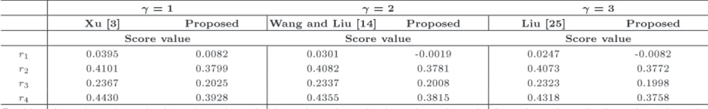
one. However, for dierent values of , say = 1; 2; 3, the score functions and an overall aggregated IVIFN for alternatives are given in Table 1 by the existing and proposed operators. From these results, it can be concluded that the results of the proposed operators coincide with the results of the existing methodologies and the obtained aggregated IVIFN is more optimistic than the aggregated values of the existing methodologies for taking a decision.

On the other hand, if we aggregate these dierent IVIFNs by IVIFHIHWA operator, then, rstly we nd

_ij= (3wj)ij as: _11=

(1:4)1:2 _(0:6)1:2 (1:4)1:2_{+ (0:6)}1:2;

(1:5)1:2 _(0:5)1:2 (1:5)1:2_{+ (0:5)}1:2

;

r1= IVIFHIWA(r11; r12; r13)

=

*_(1:4)0:25_(1:4)0:45_(1:1)0:3 _(0:6)0:25_(0:6)0:45_(0:9)0:3

(1:4)0:25_(1:4)0:45_(1:1)0:3_{+ (0:6)}0:25_(0:6)0:45_(0:9)0:3;

(1:5)0:25_(1:6)0:45_(1:3)0:3 _(0:5)0:25_(0:4)0:45_(0:7)0:3

(1:5)0:25_(1:6)0:45_(1:3)0:3_{+ (0:5)}0:25_(0:4)0:45_(0:7)0:3

; 2(0:6)0:25_(0:6)0:45_(0:9)0:3 _(0:3)0:25_(0:4)0:45_(0:4)0:3

(1:4)0:25_(1:4)0:45_(1:1)0:3_{+ (0:6)}0:25_(0:6)0:45_(0:9)0:3 ;

2(0:5)0:25_(0:4)0:45_(0:7)0:3 _(0:1)0:25_(0:0)0:45_(0:1)0:3

(1:5)0:25_(1:6)0:45_(1:3)0:3_{+ (0:5)}0:25_(0:4)0:45_(0:7)0:3

+

= h[0:3155; 0:4946]; [0:3085; 0:5054]i r2= IVIFHIWA(r21; r22; r23)

=

*_(1:6)0:25_(1:6)0:45_(1:4)0:3 _(0:4)0:25_(0:4)0:45_(0:6)0:3

(1:6)0:25_(1:6)0:45_(1:4)0:3_{+ (0:4)}0:25_(0:4)0:45_(0:6)0:3;

(1:7)0:25_(1:7)0:45_(1:7)0:3 _(0:3)0:25_(0:3)0:45_(0:3)0:3

(1:7)0:25_(1:7)0:45_(1:7)0:3_{+ (0:3)}0:25_(0:3)0:45_(0:3)0:3

; 2(0:4)0:25_(0:4)0:45_(0:6)0:3 _(0:2)0:25_(0:2)0:45_(0:5)0:3

(1:6)0:25_(1:6)0:45_(1:4)0:3_{+ (0:4)}0:25_(0:4)0:45_(0:6)0:3 ;

2

(0:3)0:25_(0:3)0:45_(0:3)0:3 _(0:0)0:25_(0:0)0:45_(0:1)0:3

(1:6)0:25_(1:6)0:45_(1:4)0:3_{+ (0:4)}0:25_(0:4)0:45_(0:6)0:3

+

= h[0:5457; 0:7000]; [0:1895; 0:3000]i r3= IVIFHIWA(r31; r32; r33)

= *

(1:3)0:25_(1:5)0:45_(1:5)0:3 _(0:7)0:25_(0:5)0:45_(0:5)0:3

(1:3)0:25_(1:5)0:45_(1:5)0:3_{+ (0:7)}0:25_(0:5)0:45_(0:5)0:3;

(1:6)0:25_(1:6)0:45_(1:6)0:3 _(0:4)0:25_(0:4)0:45_(0:4)0:3

(1:6)0:25_(1:6)0:45_(1:6)0:3_{+ (0:4)}0:25_(0:4)0:45_(0:4)0:3

; 2(0:7)0:25_(0:5)0:45_(0:5)0:3 _(0:4)0:25_(0:2)0:45_(0:4)0:3

(1:3)0:25_(1:5)0:45_(1:5)0:3_{+ (0:7)}0:25_(0:5)0:45_(0:5)0:3 ;

2(0:4)0:25_(0:4)0:45_(0:4)0:3 _(0:0)0:25_(0:0)0:45_(0:1)0:3

(1:6)0:25_(1:6)0:45_(1:6)0:3_{+ (0:4)}0:25_(0:4)0:45_(0:4)0:3

+

= h[0:4537; 0:6000]; [0:2522; 0:4000]i r4= IVIFHIWA(r41; r42; r43)

=

*_(1:7)0:25_(1:6)0:45_(1:3)0:3 _(0:3)0:25_(0:4)0:45_(0:7)0:3

(1:7)0:25_(1:6)0:45_(1:3)0:3_{+ (0:3)}0:25_(0:4)0:45_(0:7)0:3;

(1:8)0:25_(1:7)0:45_(1:4)0:3 _(0:2)0:25_(0:3)0:45_(0:6)0:3

(1:8)0:25_(1:7)0:45_(1:4)0:3_{+ (0:2)}0:25_(0:3)0:45_(0:6)0:3

; 2

(0:3)0:25_(0:4)0:45_(0:3)0:3 _(0:2)0:25_(0:3)0:45_(0:6)0:3

(1:7)0:25_(1:6)0:45_(1:3)0:3_{+ (0:2)}0:25_(0:3)0:45_(0:6)0:3 ;

2

(0:2)0:25_(0:3)0:45_(0:6)0:3 _(0:0)0:25_(0:0)0:45_(0:4)0:3

(1:8)0:25_(1:7)0:45_(1:4)0:3_{+ (0:2)}0:25_(0:3)0:45_(0:6)0:3

+

= h[0:5522; 0:6596]; [0:1084; 0:3404]i:

Table 1. Comparison with IVIFHIWA and existing operators.

= 1 = 2 = 3

Xu [3] Proposed Wang and Liu [14] Proposed Liu [25] Proposed

Score value Score value Score value

r1 0.0395 0.0082 0.0301 -0.0019 0.0247 -0.0082

r2 0.4101 0.3799 0.4082 0.3781 0.4073 0.3772

r3 0.2367 0.2025 0.2337 0.2008 0.2323 0.1998

r4 0.4430 0.3928 0.4355 0.3815 0.4318 0.3758

Ranking A4 A2 A3 A1A4 A2 A3 A1 A4 A2 A3 A1A4 A2 A3 A1A4 A2 A3 A1A2 A4 A3 A1

_R(ij)(xij0) =

2 6 6 4

h[0:4687; 0:5778]; [0:3000; 0:3610]i h[0:3075; 0:4776]; [0:1816; 0:5224]i h[0:1050; 0:3140]; [0:5130; 0:5971]i h[0:6814; 0:7782]; [0:1799; 0:2218]i h[0:4176; 0:7215]; [0:1015; 0:1907]i h[0:4776; 0:5720]; [0:2118; 0:4280]i h[0:5203; 0:6217]; [0:1002; 0:2900]i h[0:3552; 0:6814]; [0:3153; 0:3186]i h[0:3902; 0:4776]; [0:3031; 0:5224]i h[0:7782; 0:8664]; [0:0855; 0:1336]i h[0:4776; 0:5720]; [0:1014; 0:4280]i h[0:3140; 0:4176]; [0:1025; 0:2019]i 3 7 7 5 Box VIII

2f(0:6)1:2 _(0:3)1:2_g (1:4)1:2_{+ (0:6)}1:2 ;

2f(0:5)1:2 _(0:1)1:2_g (1:5)1:2_{+ (0:5)}1:2

= h[0:4687; 0:5778]; [0:3000; 0:3610]i _12=

(1:4)0:75 _(0:6)0:75 (1:4)0:75_{+ (0:6)}0:75;

(1:6)0:75 _(0:4)0:75 (1:6)0:75_{+ (0:4)}0:75

;

2f(0:6)0:75 _(0:4)0:75_g (1:4)0:75_{+ (0:6)}0:75 ;

2f(0:4)0:75 _(0:0)0:75_g (1:6)0:75_{+ (0:4)}0:75

= h[0:3075; 0:4776]; [0:1816; 0:5224]i

_13=

(1:1)1:05 _(0:9)1:05 (1:1)1:05_{+ (0:9)}1:05;

(1:3)1:05 _(0:7)1:05 (1:3)1:05_{+ (0:7)}1:05

;

2f(0:7)1:05 _(0:4)1:05_g (1:1)1:05_{+ (0:9)}1:05 ;

2f(0:7)1:05 _(0:1)1:05_g (1:3)1:05_{+ (0:7)}1:05

= h[0:0990; 0:2972]; [0:4973; 0:6004]i = h[0:1050; 0:3140]; [0:5130; 0:5971]i: Similarly:

_21= h[0:6814; 0:7782]; [0:1799; 0:2218]i; _22= h[0:4776; 0:5720]; [0:2118; 0:4280]i; _23= h[0:4176; 0:7215]; [0:1015; 0:1907]i; _31= h[0:3552; 0:6814]; [0:3153; 0:3186]i; _32= h[0:3902; 0:4776]; [0:3031; 0:5224]i; _33= h[0:5203; 0:6217]; [0:1002; 0:2900]i

_41= h[0:7782; 0:8664]; [0:0855; 0:1336]i; _42= h[0:4776; 0:5720]; [0:1014; 0:4280]i; _43= h[0:3140; 0:4176]; [0:1025; 0:2019]i:

Then by score functions, we can get _R(ij) as shown in Box VIII.

Hence, the overall performance value ri corre-sponding to each alternative, Ai, is obtained by the aggregated IVIFHIHWA operator corresponding to the weight !i = (0:25; 0:45; 0:30)T as:

r1= h[0:2929; 0:4591]; [0:3191; 0:5409]i; r2= h[0:5110; 0:6989]; [0:1772; 0:3011]i; r3= h[0:4094; 0:6121]; [0:2556; 0:3879]i; r4= h[0:5311; 0:6386]; [0:1100; 0:3614]i:

By using the score function, we get the score values of these respective alternatives as:

S(r1) = 0:0540; S(r2) = 0:3658; S(r3) = 0:1890; S(r4) = 0:3491:

Therefore, the ranking order of the four alterna-tives is A2 A4 A3 A1, i.e., food company arms company computer company car company; thus, A2(i.e., food company) is the most desirable one and A1 (i.e., car company) is the least desirable one.

In order to compare the ranking of these alter-natives with the rankings in other aggregating op-erators, namely, IVIFWA [3], IVIFEWA [14], and IVIFHWA [25], by properly assigning the value of

to a desired number, their corresponding score values and an overall aggregated IVIFN for alternatives are given in Table 2 by the existing and proposed operators. From these results, it can be concluded that the results of the proposed operator coincide with results of the existing methodologies and the obtained aggregated IVIFN is more optimistic than the aggregated values of the existing methodologies for taking a decision.

To analyze the eect of on the most desirable alternatives in the given attributes, we use dierent values of in the proposed approach to rank the alternatives. The corresponding score values and their ranking order are summarized in Table 3. From this table, it can be seen that the aggregation results by using dierent values of are dierent, but the corre-sponding rankings of the alternatives are the same. Table 2. Comparison with IVIFHIHWA and existing operators.

= 1 = 2 = 3

Xu [3] Proposed Wang and Liu [14] Proposed Liu 25 Proposed

Score value Score value Score value

r1 -0.0157 -0.0397 -0.0312 -0.0540 -0.0411 -0.0635

r2 0.4102 0.3683 0.4075 0.3658 0.4061 0.3644

r3 0.2212 0.1885 0.2216 0.1890 0.2227 0.1899

r4 0.4169 0.3679 0.4042 0.3491 0.3986 0.3384

Ranking A4 A2 A3 A1A2 A4 A3 A1A2 A4 A3 A1 A2 A4 A3 A1A2 A4 A3 A1A2 A4 A3 A1

Table 3. Ordering of the attributes for dierent values of .

By IVIFHIWA By IVIFHIOWA By IVIFHIHWA

Aggregated IVIFN Score

values Aggregated IVIFN

Score

values Aggregated IVIFN

Score values A1 h[0:3319; 0:5108]; [0:3011; 0:4892]i 0.0262 h[0:3319; 0:4862][0:3216; 0:5138]i -0.0086 h[0:3134; 0:4820]; [0:3099; 0:5180]i -0.0162

A2 h[0:5542; 0:7000]; [0:1860; 0:3000]i 0.3841 h[0:5542; 0:7000][0:1860; 0:3000]i 0.3841 h[0:5226; 0:6994]; [0:1730; 0:3006]i 0.3742

0.1 A3 h[0:4607; 0:6000]; [0:2489; 0:4000]i 0.2059 h[0:4522; 0:6000][0:2578; 0:4000]i 0.1972 h[0:4171; 0:6070]; [0:2522; 0:3930]i 0.1894

A4 h[0:5771; 0:6863]; [0:1023; 0:3137]i 0.4237 h[0:5771; 0:6863]; [0:1023; 0:3137]i 0.4237 h[0:5675; 0:6792]; [0:1014; 0:3208]i 0.4123

Ranking A4 A2 A3 A1 A4 A2 A3 A1 A4 A2 A3 A1

A1 h[0:3271; 0:5045]; [0:3032; 0:4955]i 0.0164 h[0:3271; 0:4809]; [0:3239; 0:5191]i -0.0175 h[0:3074; 0:4738]; [0:3126; 0:5262]i -0.0288

A2 h[0:5507; 0:7000]; [0:1874; 0:3000]i 0.3816 h[0:5507; 0:7000]; [0:1874; 0:3000]i 0.3816 h[0:5178; 0:6992]; [0:1748; 0:3008]i 0.3707

0.5 A3 h[0:4582; 0:6000]; [0:2501; 0:4000]i 0.2040 h[0:4493; 0:6000]; [0:2592; 0:4000]i 0.1950 h[0:4140; 0:6085]; [0:2536; 0:3915]i 0.1887

A4 h[0:5668; 0:6736]; [0:1048; 0:3264]i 0.4046 h[0:5668; 0:6736]; [0:1048; 0:3264]i 0.4046 h[0:5533; 0:6613]; [0:1048; 0:3387]i 0.3855

Ranking A4 A2 A3 A1 A4 A2 A3 A1 A4 A2 A3 A1

A1 h[0:3224; 0:4997]; [0:3054; 0:5003]i 0.0082 h[0:3224; 0:4769]; [0:3262; 0:5231]i -0.0250 h[0:3015; 0:4672]; [0:3152; 0:5328]i -0.0397

A2 h[0:5483; 0:7000]; [0:1885; 0:3000]i 0.3799 h[0:5483; 0:7000]; [0:1885; 0:3000]i 0.3799 h[0:5144; 0:6991]; [0:1760; 0:3009]i 0.3683

1 A3 h[0:4561; 0:6000]; [0:2511; 0:4000]i 0.2025 h[0:4469; 0:6000]; [0:2603; 0:4000]i 0.1933 h[0:4117; 0:6100]; [0:2546; 0:3900]i 0.1885

A4 h[0:5597; 0:6663]; [0:1065; 0:3337]i 0.3928 h[0:5597; 0:6663]; [0:1065; 0:3337]i 0.3928 h[0:5429; 0:6501]; [0:1072; 0:3499]i 0.3679

Ranking A4 A2 A3 A1 A4 A2 A3 A1 A4 A2 A3 A1

A1 h[0:3155; 0:4946]; [0:3085; 0:5054]i -0.0019 h[0:3155; 0:4725]; [0:3295; 0:5274]i -0.0344 h[0:2929; 0:4591]; [0:3191; 0:5409]i -0.0540

A2 h[0:5457; 0:7000]; [0:1895; 0:3000]i 0.3781 h[0:5457; 0:7000]; [0:1895; 0:3000]i 0.3781 h[0:5110; 0:6989]; [0:1772; 0:3011]i 0.3658

2 A3 h[0:4537; 0:6000]; [0:2522; 0:4000]i 0.2008 h[0:4441; 0:6000]; [0:2616; 0:4000]i 0.1913 h[0:4094; 0:6121]; [0:2556; 0:3879]i 0.1890

A4 h[0:5522; 0:6596]; [0:1084; 0:3404]i 0.3815 h[0:5522; 0:6596]; [0:1084; 0:3404]i 0.3815 h[0:5311; 0:6386]; [0:1100; 0:3614]i 0.3491

Ranking A4 A2 A3 A1 A4 A2 A3 A1 A2 A4 A3 A1

A1 h[0:3043; 0:4888]; [0:3135; 0:5112]i -0.0158 h[0:3043; 0:4676]; [0:3349; 0:5324]i -0.0477 h[0:2782; 0:4479]; [0:3258; 0:5521]i -0.0759

A2 h[0:5431; 0:7000]; [0:1906; 0:3000]i 0.3763 h[0:5431; 0:7000]; [0:1906; 0:3000]i 0.3763 h[0:5074; 0:6986]; [0:1785; 0:3014]i 0.3630

5 A3 h[0:4508; 0:6000]; [0:2535; 0:4000]i 0.1987 h[0:4408; 0:6000]; [0:2631; 0:4000]i 0.1889 h[0:4080; 0:6158]; [0:2562; 0:3842]i 0.1917

A4 h[0:5441; 0:6532]; [0:1103; 0:3468]i 0.3701 h[0:5441; 0:6532]; [0:1103; 0:3468]i 0.3701 h[0:4978; 0:6101]; [0:1147; 0:3899]i 0.3016

Ranking A2 A4 A3 A1 A2 A4 A3 A1 A2 A4 A3 A1

A1 h[0:2961; 0:4859]; [0:3172; 0:5141]i -0..0247 h[0:2961; 0:4651]; [0:3388; 0:5349]i -0.0562 h[0:2667; 0:4395]; [0:3310; 0:5605]i -0.0926

A2 h[0:5419; 0:7000]; [0:1911; 0:3000]i 0.3754 h[0:5419; 0:7000]; [0:1911; 0:3000]i 0.3754 h[0:5055; 0:6982]; [0:1792; 0:3018]i 0.3614

10 A3 h[0:4493; 0:6000]; [0:2542; 0:4000]i 0.1975 h[0:4391; 0:6000]; [0:2640; 0:4000]i 0.1876 h[0:4086; 0:6193]; [0:2559; 0:3807]i 0.1957

A4 h[0:5401; 0:6504]; [0:1113; 0:3496]i 0.3648 h[0:5401; 0:6504]; [0:1113; 0:3496]i 0.3648 h[0:4918; 0:6056]; [0:1160; 0:3944]i 0.2935

Ranking A2 A4 A3 A1 A2 A4 A3 A1 A2 A4 A3 A1

A1 h[0:2882; 0:4837]; [0:3208; 0:5163]i -0.0326 h[0:2882; 0:4633]; [0:3426; 0:5367]i -0.0639 h[0:2533; 0:4290]; [0:3370; 0:5710]i -0.1129

A2 h[0:5411; 0:7000]; [0:1915; 0:3000]i 0.3748 h[0:5411; 0:7000]; [0:1915; 0:3000]i 0.3748 h[0:5040; 0:6978]; [0:1798; 0:3022]i 0.3599

25 A3 h[0:4481; 0:6000]; [0:2547; 0:4000]i 0.1967 h[0:4378; 0:6000]; [0:2646; 0:4000]i 0.1866 h[0:4116; 0:6244]; [0:2546; 0:3756]i 0.2029

A4 h[0:5372; 0:6485]; [0:1120; 0:3515]i 0.3611 h[0:5372; 0:6485]; [0:1120; 0:3515]i 0.3611 h[0:4872; 0:6023]; [0:1171; 0:3977]i 0.2874

Ranking A2 A4 A3 A1 A2 A4 A3 A1 A2 A4 A3 A1

A1 h[0:2846; 0:4829]; [0:3224; 0:5171]i -0.0360 h[0:2846; 0:4626]; [0:3444; 0:5374]i -0.0673 h[0:2450; 0:4211]; [0:3407; 0:5789]i -0.1267

A2 h[0:5408; 0:7000]; [0:1916; 0:3000]i 0.3746 h[0:5408; 0:7000]; [0:1916; 0:3000]i 0.3746 h[0:5032; 0:6975]; [0:1800; 0:3025]i 0.3591

50 A3 h[0:4477; 0:6000]; [0:2549; 0:4000]i 0.1964 h[0:4373; 0:6000]; [0:2648; 0:4000]i 0.1863 h[0:4150; 0:6286]; [0:2532; 0:3714]i 0.2095

A4 h[0:5361; 0:6478]; [0:1123; 0:3522]i 0.3597 h[0:5361; 0:6478]; [0:1123; 0:3522]i 0.3597 h[0:4854; 0:6009]; [0:1175; 0:3991]i 0.2849