Transmuted Modified Weibull Distribution: A Generalization of the Modified Weibull Probability Distribution

Vol. 6, No. 1, 2013, 66-88

ISSN 1307-5543 – www.ejpam.com

Transmuted Modified Weibull Distribution: A Generalization

of the Modified Weibull Probability Distribution

Muhammad Shuaib Khan

, Robert King

School of Mathematical and Physical Sciences, The University of Newcastle, Callaghan, NSW 2308, Australia

Abstract. This paper introduces a transmuted modified Weibull distribution as an important compet-itive model which contains eleven life time distributions as special cases. We generalized the three parameter modified Weibull distribution using the quadratic rank transmutation map studied by Shaw et al. [12]to develop a transmuted modified Weibull distribution. The properties of the transmuted modified Weibull distribution are discussed. Least square estimation is used to evaluate the parame-ters. Explicit expressions are derived for the quantiles. We derive the moments and examine the order statistics. We propose the method of maximum likelihood for estimating the model parameters and obtain the observed information matrix. This model is capable of modeling of various shapes of aging and failure criteria.

2010 Mathematics Subject Classifications: 90B25; 62N05

Key Words and Phrases: Reliability functions, moment estimation, moment generating function, least square estimation, order statistics, maximum likelihood estimation.

1. Introduction

The Weibull distribution is a life time probability distribution used in the reliability engi-neering discipline. We introduce the transmuted modified Weibull distribution which extends recent development on transmuted Weibull distribution by Aryal et al. [1]. More recently Aryal et al. [2] introduced the transmuted extreme value distribution. In this article, we introduce and study several mathematical properties of new reliability model referred to as the transmuted modified Weibull distribution. This paper focuses on all the properties of this model and presents the graphical analysis of the subject distribution. This paper presents the relationship between shape parameter and other properties such as non-reliability function, reliability function, instantaneous failure rate, cumulative instantaneous failure rate models. Recently Ammar et al.[10]proposed the modified Weibull distribution.

F_{M W}(t) =1−exp(₋αt−ηtβ). (1)

∗_{Corresponding author.}

Email addresses:Shuaib.statgmail.om(M. Shuaib),robert.kingnewastle.edu.au(R. King)

This article defined the family of transmuted modified Weibull distributions. The main fea-ture of this model is that a transmuted parameterλ is introduced in the subject distribution which provides greater flexibility in the form of new distributions. Using the quadratic rank transmutation map studied by Shaw et al. [12], we develop the four parameter transmuted modified Weibull distribution T M W D(α,β,η,λ,t). We provide a comprehensive description of mathematical properties of the subject distribution with the hope that it will attract wider applications in reliability, engineering and in other areas of research. These distributions have several attractive properties for more details we refer to[5, 8, 4, 6, 7, 13].

The article is organized as follows, In Section 2, we present the flexibility of the subject distribution and some special sub-models. In Section 3, we demonstrate the reliability func-tions of the subject model. A range of mathematical properties are considered in Section 4-5. These include quantile functions, moment estimation, moment generating function and least square estimation. In Section 6, the minimum, maximum and median order statistics models are discussed. We also demonstrate the joint density functions g(t₁,t_n)of the trans-muted modified Weibull distribution. In Section 7, we demonstrate the maximum likelihood estimates(M LE_S)of the unknown parameters and the asymptotic confidence intervals of the unknown parameters. However, some of these quantities could not be evaluated in closed form and therefore special cases were used to express them. In Section 8, we fit the TMW model to illustrate its usefulness. In Section 9, concluding remarks are addressed.

2. Transmuted Modified Weibull Distribution

A random variable T is said to have transmuted Modified Weibull probability distribu-tion with parameters α,β,η > 0 and−1≤ λ ≤1 . It can be used to represent the failure probability density function is given by

fT M W(t) = (α+β ηtβ−1)exp(−αt−ηtβ)(1−λ+2λexp(−αt−ηtβ)) t >0 (2) Whereβandηare the shape parameters representing the different patterns of the trans-muted modified Weibull distribution and are positive,αis a scale parameter representing the characteristic life and is also positive,λis the transmuted parameter. The restrictions in equa-tion (2) on the values ofα,β,ηandλare always the same.

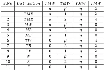
The transmuted modified Weibull distribution is very flexible model that approaches to different distributions when its parameters are changed. The flexibility of the transmuted modified Weibull distribution is explained in Table 1. The subject distribution includes as special cases the transmuted modified Exponential (TME), transmuted Linear Failure Rate (TLFR), transmuted Weibull (TW), transmuted Rayleigh (TR) and transmuted Exponential distributions. Figure 1 shows the transmuted modified Weibull distribution that approaches to eleven different lifetime distributions when its parameters are changed. The cumulative distribution function of the transmuted modified Weibull distribution is denoted byF_{T M W}(t)

and is defined as

Figure 1: Sub Models of Transmuted Modified Weibull Distribution

Table 1: Modified and Transmuted Modified type distributions: T=Transmuted; M=Modified; W=Weibull; E=Exponential; R=Rayleigh

S.N o Dist r i bution T M W T M W T M W T M W

α β η λ

1 T M E α 1 η λ

2 T M R α 2 η λ

3 M W α β η 0

4 M R α 2 η 0

5 M E α 1 η 0

6 T W 0 β η λ

7 T R 0 2 η λ

8 T E 0 1 η λ

9 W 0 β η 0

10 R 0 2 η 0

11 E 0 1 η 0

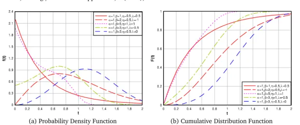
Figure 2a shows the diverse shape of the transmuted modified Weibull PDF with different choice of parameters. The beauty of the subject distribution and its sub models are explained in Table 1.

(a) Probability Density Function (b) Cumulative Distribution Function

Figure 2: Transmuted Modified Weibull PDF & CDF

3. Reliability Analysis

The transmuted modified Weibull distribution can be a useful characterization of life time data analysis. The reliability function (RF) of the transmuted modified Weibull distribution is denoted byR_{T M W}(t)also known as the survivor function and is defined as

RT M W(t) =1−FT M W(t)

RT M W(t) =1−(1−exp(−αt−ηtβ))(1+λexp(−αt−ηtβ)) (4) It is important to note that R_{T M W}(t) +F_{T M W}(t) = 1 . Figure 3a illustrates the reliability pattern of the transmuted modified Weibull distribution with different choice of parameters. One of the characteristic in reliability analysis is the hazard rate function defined by

h_{T M W}(t) = fT M W(t)

1₋FT M W(t)

(5)

The hazard function (HF) of the transmuted modified Weibull distribution also known as instantaneous failure rate denoted byh_{T M W}(t)and is defined as fT M W(t)

RT M W(t)

h_{T M W}(t) = (α+β ηt

β−1_{)exp(−αt−ηt}β_{)(1−λ+2λexp(−αt−ηt}β₎₎

1₋(1₋exp(₋αt₋ηtβ_{))(1+λexp(−αt−ηt}β₎₎ (6) It is important to note that the units forhT M W(t)is the probability of failure per unit of time, distance or cycles.

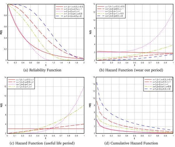
(a) Reliability Function (b) Hazard Function (wear out period)

(c) Hazard Function (useful life period) (d) Cumulative Hazard Function

Figure 3: Transmuted Modified Weibull Reliability and Hazard Functions

In both cases when β = 5 the distribution has the strictly increasing HR. whenβ = 1 , the HR is steadily increasing in Figure 3b which represents failure life between early failures and wear out periods. Whenβ =1 , the HR is constant in Figure 3c which represents failure life in useful life period. When β > 1 , the HF is continually increasing which represents failures occurs after the useful life periods and approaches to the wear-out failures. The HR of the TMWD as given in equation (6) becomes identical with the HR of transmuted modified Rayleigh distribution for β = 2 and for β = 1 it coincides with the transmuted modified Exponential distribution. So the transmuted modified Weibull distribution is a very flexible reliability model.

The Cumulative hazard function of the transmuted modified Weibull distribution is de-noted byH_{T M W}(t)and is defined as

hazard failure rates with different choices of parameters. For all choice of parameters the distribution has the decreasing patterns of cumulative instantaneous failure rates.

Theorem 1. The hazard rate function of the transmuted modified Weibull distribution has the following properties

(i) Ifβ=1the failure rate is same as the T M E D(α,η,λ,t)

(ii) Ifβ=2the failure rate is same as the T LF RD(α,η,λ,t)

(iii) Ifα=0the failure rate is same as the T W D(β,η,λ,t)

(iv) Ifα=0,β=1the failure rate is same as the T E D(η,λ,t)

(v) Ifα=0,β=2the failure rate is same as the T RD(η,λ,t)

(vi) Ifλ=0the failure rate is same as the M W D(α,β,η,t)

(vii) Ifλ=0,β=1the failure rate is same as the M E D(α,η,t)

(viii) Ifλ=0,β=2the failure rate is same as the M RD(α,η,t)

Proof. The hazard function (HF) of the transmuted modified Weibull distribution is given in equation (6) has the special cases with different choice of parameters

(i) Ifβ=1 the failure rate is same as theT M E D(α,η,λ,t)

h_{T M E}(t) =(α+η)exp(−αt−ηt)(1−λ+2λexp(−αt−ηt))

1₋(1₋exp(₋αt−ηt))(1+λexp(₋αt−ηt))

(ii) Ifβ=2 the failure rate is same as theT LF RD(α,η,λ,t)

h_{T L F R}(t) = (α+2ηt)exp(−αt−ηt

2_{)(1−λ+2λexp(−αt−ηt}2₎₎

1−(1−exp(−αt−ηt2_{))(1+λexp(−αt−ηt}2₎₎

(iii) Ifα=0 the failure rate is same as theT W D(β,η,λ,t)

h_{T W}(t) = (β ηt

β−1_)exp(−ηtβ_{)(1−λ+2λexp(−ηt}β₎₎ 1₋(1₋exp(₋ηtβ))(1+λexp(₋ηtβ))

(iv) Ifα=0,β=1 the failure rate is same as theT E D(η,λ,t)

h_{T E}(t) = (η)exp(−ηt)(1−λ+2λexp(−ηt))

1−(1−exp(₋ηt))(1+λexp(₋ηt))

(v) Ifα=0,β=2 the failure rate is same as theT RD(η,λ,t)

h_{T R}(t) = (2ηt)exp(−ηt

2_{)(1−λ+2λexp(−ηt}2₎₎

(vi) Ifλ=0 the failure rate is same as theM W D(α,β,η,t)

hM W(t) =

(α+β ηtβ−1)exp(−αt−ηtβ)

1−(1−exp(−αt−ηtβ₎₎

(vii) Ifλ=0,β=1 the failure rate is same as theM E D(α,η,t)

h_{M E}(t) = (α+η)exp(−αt−ηt)

1−(1−exp(₋αt−ηt))

(viii) Ifλ=0,β=2 the failure rate is same as theM RD(α,η,t)

h_{M R}(t) = (α+2ηt)exp(−αt−ηt

2₎

1−(1−exp(₋αt−ηt2))

4. Statistical Properties

This section explain the statistical properties of the T M W D(α,β,η,λ,t)

4.1. Quantile and Median

The quantile t_qof theT M W D(α,β,η,λ,t)is the real solution of the following equation

ηt_qβ+αtq+ln



1−

(1+λ)₋p(1+λ)2_−4λq

2λ



=0 (8)

The above equation (8) has no closed-form solution in t_q, so we have different cases by sub-stituting the parametric values in the above quantile equation. So the derived special cases are

(1) The q-th quantile of theT LF RD(α,η,λ,t)by substitutingβ=2

tq=

−α+

Ç

α2−4ηln



1−(1+λ)−

p

(1+λ)2_−4λq 2λ

‹

2η

(2) The q-th quantile of theT W D(β,η,λ,t)by substitutingα=0

t_q=



−

1

ηln



1−

(1+λ)₋p(1+λ)2_−4λq

2λ



 

 1

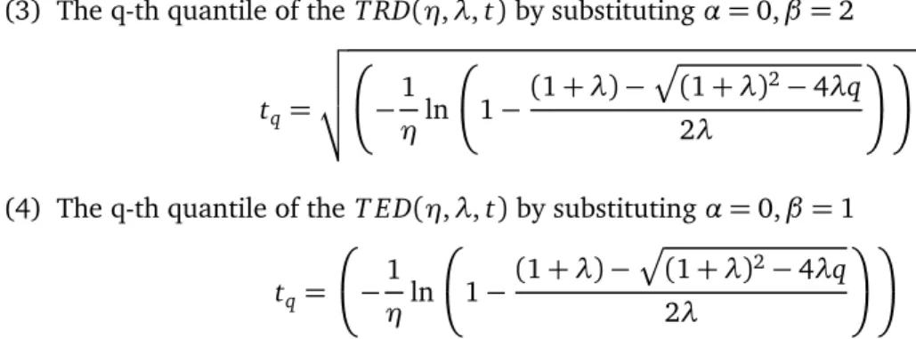
(3) The q-th quantile of theT RD(η,λ,t)by substitutingα=0,β=2

tq=

v u u t



−

1

ηln



1−

(1+λ)₋p(1+λ)2_−4λq

2λ



 



(4) The q-th quantile of theT E D(η,λ,t)by substitutingα=0,β=1

t_q=



−

1

ηln



1−

(1+λ)−p(1+λ)2_−4λq

2λ



 



By puttingq=0.5 in equation (8) we can get the median ofT M W D(α,β,η,λ,t).

The median life of the subject distribution is the 50th percentile. In practice, this is the life by which 50 percent of the units will be expected to have failed and so it is the life at which 50 percent of the units would be expected to still survive. Figure 4a shows the trans-muted modified Weibull median life with different choice of parameters are 0.1 ≤ β ≤ 5,

λ = 0.3, 0.5, 0.7, 1 and the value of η = 2. It is important to note that as the λ increases the pattern of the median life increases. Figure 4b shows the multiple patterns of the sub-ject distribution for B-life with different choice of parameters. Here the B−0.1 life shows the maximum values of percentiles life and B−0.00001 life shows the minimum values of percentiles life. So as the percentile decreases the pattern of B-lives decreases. All of these B-lives are of increasing patterns. Here asβ→ ∞then these B-lives are also increasing. The subject distribution for percentile life is applying in those situations where the B-lives are of increasing order.

(a) Median (b) B-lives

Figure 4: Transmuted Modified Weibull Quantiles

4.2. Random Number Generation

The random number ast of the T M W D(α,β,η,λ,t)is defined by the following equation

ηtβ +αt+ln



1−

(1+λ)−p(1+λ)2_−4λξ

2λ



=0 (9)

The above equation is not in closed form solution in t, Usingξa random number uni-formly distributed from zero to one, we have solved the above equationF(t) =ξto obtain a random number int.

4.3. Moments

The following theorem gives the kthmoment of theT M W D(α,β,η,λ,t)

Theorem 2. If T has the T M W D(α,β,η,λ,t) with|λ_{| ≥}1, then the kthmoment of T sayµ_k

is given as follows

µ_k=

         P∞

i=0

(−1)i_ηi

i! h

(1−λ)Γ(iβ+k+1)

αiβ+k +

βηΓ(β(i+1)+k) αβ(i+1)+k

i

ifα,β,η >0

+2λP∞_i=0(−1)i(2η)i

i!

h_{αΓ(iβ+k+1)}

(2α)iβ+k+1 +

βηΓ(β(i+1)+k) (2α)β(i+1)+k

i

η− k β _Γ

1+_βk (1−λ) +λ2−

k β

‹

ifα=0

α−kΓ(1+k)((1−λ) +λ2−k) ifβ=0

(10)

Based on the above results given in Theorem 2, the coefficient of variation, coefficient of skewness and coefficient of kurtosis of T M W D can be obtained according to the following relation

C V_{T M W} =

r

µ₂

µ₁−1 (11)

C S_{T M W} =µ3−3µ2µ1+2µ

3 1

(µ₂−µ2₁)32

(12)

C K_{T M W} =µ4−4µ3µ1+6µ2µ

2 1−3µ41

(µ₂₋µ2₁)2 (13)

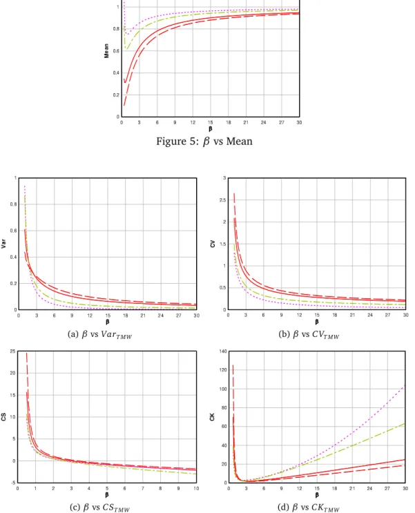
Figure 5:β vs Mean

(a)βvsVarT M W (b)βvsC VT M W

(c)βvsC ST M W (d)βvsC KT M W

Figure 6: Transmuted Modified Weibullβvs. Coefficients

measure the skewness of the distribution. The relationship betweenβandC.S_{T M W} is shown in Figure 6c. From our calculations it is clear thatC.S_{T M W} becomes asymptotically decreasing as β _{→ ∞} . Here C.K_{T M W} is the quantity used to measure the kurtosis of the distribution. The relationship betweenβ and C.K_{T M W} is shown in Figure 6d. From our calculations it is clear that asβ→ ∞the value ofC.K_{T M W} becomes asymptotically decreasing.

4.4. Moment Generating Function

The following theorem gives the moment generating function (mgf) ofT M W D(α,β,η,λ,t)

Theorem 3. If T has the T M W D(α,β,η,λ,t) with |λ| ≥ 1 , then the moment generating function of T say M_x(t)is given as follows

Mx(t) =

           P∞

i=0

(−1)i_ηi

i! h

(1−λ)₍αΓ(iβ+1)

α−t)iβ+1+

βηΓ(β(i+1)) (α−t)β(i+1)

i

ifα,β,η >0

+2λP∞_i=0 (−1)i(2η)i

i!

h _αΓ(iβ+1)

(2α−t)iβ+1+

βηΓ(β(i+1)+k) (2α−t)β(i+1)

i

P∞

i=0

ti

i!η

−i β _Γ

1+_βi (1−λ) +λ2−

i β

‹

ifα=0

α1_α−₋λ_t +₂2αλ−t

ifβ=0

(14)

The proof of this theorem is provided in Appendix. Based on the above results given in Theorem 3, the measure of central tendency, measure of dispersion, coefficient of variation, coefficient of skewness and coefficient of kurtosis of T M W D(α,β,η,λ,t) can be obtained according to the above relation in Theorem 2.

5. Least Square Estimation

LetT₁,T₂, . . . ,T_nbe a random sample ofT M W D(α,β,η,λ,t)transmuted modified Weibull distribution with cdf FT M W(t), and suppose that T(i),i=1, 2, . . . ,ndenote the ordered

sam-ple. For sample of size n, we have

E(F(T(i))) =

i n+1 The least square estimators (LSES) are obtained by minimizing

Q(α,β,η,λ) =

n

X

i=0

F(T_(i))− i

n+1

2

(15)

By using (3) and (15) we have the following equation

Q(α,β,η,λ) =

n

X

i=0

(1−exp(−αt−ηtβ))(1+λexp(−αt−ηtβ))− i

n+1

2

To minimize equation (16) with respect toα,β,ηandλ, we differentiate with respect to these parameters, which leads to the following equations

n

X

i=0

((1−exp(−αt−ηtβ))

1+λexp(−αt−ηtβ))− i

n+1

(t)

×((1+λ)exp(₋αt₋ηtβ))₋2λ(1₋exp(₋αt₋ηtβ)) =0

n

X

i=0

((1−exp(−αt−ηtβ))

1+λexp(−αt−ηtβ))− i

n+1

ηtβln(t)

×((1+λ)exp(₋αt−ηtβ))₋2λ(1₋exp(₋αt−ηtβ)) =0

n

X

i=0

((1₋exp(₋αt₋ηtβ))

1+λexp(₋αt₋ηtβ))₋ i

n+1

tβ

×((1+λ)exp(₋αt−ηtβ))₋2λ(1−exp(₋αt−ηtβ)) =0

n

X

i=0

((1−exp(₋αt−ηtβ))

1+λexp(₋αt−ηtβ))₋ i

n+1

×(exp(−αt−ηtβ))−2(1−exp(−αt−ηtβ)) =0

6. Order Statistics

Let T_1:n ≤T_2:n ≤. . .≤ T_n:n be the order statistics from the continuous distribution, then the pdf ofT_r:n 1≤r≤nis given by

f_r:n(t) =C_r:n(F(t))r−1(1−F(t))n−rf(t), t>0 (17) The joint pdf ofT_r:nandTs:n1≤r≤s≤n, is given by

fr:s:n(t,u) =Cr:s:n(F(t))r−1(F(u)−F(t))s−r−1(1−F(t))n−sf(t)f(u), (18) for 0_≤t_≤u_{≤ ∞}and whereC_r:n=₍ n!

r−1)!(n−r)! andCr:s:n=

n!

(r−1)!(s−r−1)!(n−s)!

6.1. Distribution of Minimum and Maximum

Theorem 4. Let t1,t2, . . .tnare independently identically distributed ordered random variables from the transmuted modified Weibull distribution having Ist order and nth order probability density function is given by

f1:n(t) =n(1−(1−exp(−αt−ηtβ))(1+λexp(−αt−ηtβ)))n−1(α

+β ηtβ−1)×exp(−αt−ηtβ)(1−λ+2λexp(−αt−ηtβ)) (19)

f_n:n(t) =n((1−exp(₋αt−ηtβ))(1+λexp(₋αt−ηtβ)))n−1(α+β ηtβ−1)

×exp(−αt−ηtβ)(1−λ+2λexp(−αt−ηtβ)) (20)

Proof. For the minimum and maximum order statistic of the four parameters transmuted modified Weibull distribution have different life time distributions when its parameters are changed.

Case A: Minimum order statistic

1. The minimum order statistic of theT LF RD(α,η,λ,t)by substitutingβ=2 f_1:n(t) =n(1₋(1₋exp(₋αt₋ηt2))(1+λexp(₋αt₋ηt2)))n−1(α+2ηt)

×exp(−αt−ηt2)(1−λ+2λexp(−αt−ηt2))

2. The minimum order statistic of theT M E D(α,η,λ,t)by substitutingβ=1 f1:n(t) =n(1−(1−exp(−αt−ηt))(1+λexp(−αt−ηt)))n−1(α+η)

×exp(−αt−ηt)(1−λ+2λexp(−αt−ηt))

3. The minimum order statistic of theT W D(β,η,λ,t)by substitutingα=0 f1:n(t) =n(1−(1−exp(−ηtβ))(1+λexp(−ηtβ)))n−1(β ηtβ−1)

×exp(₋ηtβ)(1−λ+2λexp(₋ηtβ))

4. The minimum order statistic of theT RD(η,λ,t)by substitutingα=0,β=2 f_1:n(t) =n(1₋(1₋exp(₋ηt2))(1+λexp(₋ηt2)))n−1(2ηt)

×exp(−ηt2)(1−λ+2λexp(−ηt2))

5. The minimum order statistic of theT E D(η,λ,t)by substitutingα=0,β=1

f_1:n(t) =n(1₋(1₋exp(₋ηt))(1+λexp(₋ηt)))n−1(η)_×exp(₋ηt)(1₋λ+2λexp(₋ηt))

7. The minimum order statistic of theM RD(α,η,t)by substitutingβ=2,λ=0, f1:n(t) =n(1−(1−exp(−αt−ηt2)))n−1(α+2ηt)exp(−αt−ηt2)

8. The minimum order statistic of theM E D(α,η,t) by substitutingβ=1,λ=0, f_1:n(t) =n(1−(1−exp(−αt−ηt)))n−1(α+η)exp(−αt−ηt)

Case B: Maximum order statistic

1. The maximum order statistic of theT LF RD(α,η,λ,t)by substitutingβ=2 f_n:n(t) =n((1₋exp(₋αt₋ηt2))(1+λexp(₋αt₋ηt2)))n−1(α+2ηt)

×exp(−αt−ηt2)(1−λ+2λexp(−αt−ηt2))

2. The maximum order statistic of theT M E D(α,η,λ,t) by substitutingβ=1 f_n:n(t) =n((1−exp(−αt−ηt))(1+λexp(−αt−ηt)))n−1(α+η)

×exp(−αt−ηt)(1−λ+2λexp(−αt−ηt))

3. The maximum order statistic of theT W D(β,η,λ,t)by substitutingα=0 f_n:n(t) =n((1−exp(−ηtβ))(1+λexp(−ηtβ)))n−1(β ηtβ−1)

×exp(₋ηtβ)(1₋λ+2λexp(₋ηtβ))

4. The maximum order statistic of theT RD(η,λ,t)by substitutingα=0,β=2 fn:n(t) =n((1−exp(−ηt2))(1+λexp(−ηt2)))n−1(2ηt)

×exp(−ηt2)(1−λ+2λexp(−ηt2))

5. The maximum order statistic of theT E D(η,λ,t)by substitutingα=0,β=1

fn:n(t) =n((1−exp(−ηt))(1+λexp(−ηt)))n−1(η)×exp(−ηt)(1−λ+2λexp(−ηt))

6. The maximum order statistic of theM W D(α,β,η,t)by substitutingλ=0, fn:n(t) =n((1−exp(−αt−ηtβ)))n−1(α+β ηtβ−1)exp(−αt−ηtβ)

8. The maximum order statistic of theM E D(α,η,t)by substitutingβ=1,λ=0, fn:n(t) =n((1−exp(−αt−ηt)))n−1(α+η)exp(−αt−ηt)

Theorem 5. Let t1,t2, . . .tnare independently identically distributed ordered random variables from the transmuted modified Weibull distribution having median order T_m+1probability density

function is given by

g(˜t) = (2m+1)!

m!m! (F(˜t))

m_(1−F(˜t))m_{f(˜t), 0≤˜t ≤ ∞ (21)}

Proof. Using (21) the median order statistic of the four parameters transmuted modified Weibull distribution is given below

g(˜t) =(2m+1)!

m!m! ((1−exp(−α˜t−η˜t

β_{))(1+λexp(−α˜t−η˜t}β₎₎₎m_{(α+β η˜t}β−1₎

×(1−(1−exp(₋α˜t−η˜tβ))(1+λexp(₋α˜t−η˜tβ)))m

×exp(−α˜t−η˜tβ)(1−λ+2λexp(−α˜t−η˜tβ)) (22)

Using (22) we have different life time distributions of median order statistic when its param-eters are changed

1. The median order statistic of theT LF RD(α,η,λ,t) by substitutingβ=2

g(˜t) =(2m+1)!

m!m! ((1−exp(−α˜t−η˜t

2_{))(1+λexp(−α˜t−η˜t}2₎₎₎m_(α+2η˜t)

×(1−(1−exp(−α˜t−η˜t2))(1+λexp(−α˜t−η˜t2)))m

×exp(₋α˜t−η˜t2)(1−λ+2λexp(₋α˜t−η˜t2))

2. The median order statistic of theT M E D(α,η,λ,t) by substitutingβ=1

g(˜t) =(2m+1)!

m!m! ((1−exp(−α˜t−η˜t))(1+λexp(−α˜t−η˜t)))

m_(α+η)

×(1−(1−exp(−α˜t−η˜t))(1+λexp(−α˜t−η˜t)))m

×exp(₋α˜t−η˜t)(1−λ+2λexp(₋α˜t−η˜t))

3. The median order statistic of theT W D(β,η,λ,t)by substitutingα=0

g(˜t) =(2m+1)!

m!m! ((1−exp(−η˜t

β_{))(1+λexp(−η˜t}β₎₎₎m_{(β η˜t}β−1₎

×(1−(1−exp(−η˜tβ))(1+λexp(−η˜tβ)))m

4. The median order statistic of theT RD(η,λ,t)by substitutingα=0,β=2

g(˜t) =(2m+1)!

m!m! ((1−exp(−η˜t

2_{))(1+λexp(−η˜t}2₎₎₎m_(2η˜t)

×(1₋(1₋exp(₋η˜t2))(1+λexp(₋η˜t2)))m

×exp(−η˜t2)(1−λ+2λexp(−η˜t2))

5. The median order statistic of theT E D(η,λ,t)by substitutingα=0,β=1

g(˜t) =(2m+1)!

m!m! ((1−exp(−η˜t))(1+λexp(−η˜t))) m_(η˜t)

×(1₋(1₋exp(₋η˜t))(1+λexp(₋η˜t)))m

×exp(₋η˜t)(1₋λ+2λexp(₋η˜t))

6. The median order statistic of theM W D(α,β,η,t)by substitutingλ=0,

g(˜t) =(2m+1)!

m!m! ((1−exp(−α˜t−η˜t

β₎₎m_{(α+β η˜t}β−1₎

×(1−(1−exp(₋α˜t−ηt˜β))m_×exp(₋α˜t−η˜tβ)

7. The median order statistic of theM RD(α,η,t) by substitutingβ=2,λ=0,

g(˜t) =(2m+1)!

m!m! ((1−exp(−α˜t−η˜t

2₎₎m_(α+2η˜t)

×(1−(1−exp(₋α˜t−η˜t2))m_×exp(₋α˜t−η˜t2)

8. The median order statistic of theM E D(α,η,t)by substitutingβ=1,λ=0,

g(˜t) =(2m+1)!

m!m! ((1−exp(−α˜t−η˜t))

m_(α+η)

×(1−(1−exp(−α˜t−η˜t))m×exp(−α˜t−η˜t)

6.2. Joint Distribution of rth Order Statistic

T

and sth Order Statistic

T

The joint pdf ofTr andTs with Tr=t andTs=u, (1≤r≤s≤n) in (18) by taking r=1 ands=nin (17) the minimum and maximum joint density can be written as

g(t₁,t_n) =n(n−1)(F(t_n)−F(t₁))n−2f(t₁)f(t₂) (23) Theorem 6. Let t₁,t₂, . . . ,t_n be independently identically distributed ordered random variables from the transmuted modified Weibull distribution having joint probability density function using (2)and(3)in(23)is given by

g(t1,tn) =n(n−1)(α+β ηt β−1

1 )exp(−αt1−ηt

β

1)(1−λ+2λexp(−αt1−ηt

β

×(α+β ηtβ_n−1)exp(−αt_n−ηt_nβ)(1−λ+2λexp(−αt_n−ηtβ_n))

×[(1−exp(−αt_n−ηtβ_n))(1+λexp(−αt_n−ηtβ_n))

−(1−exp(−αt₁−ηtβ₁))(1+λexp(−αt₁−ηtβ₁))]n−2 (24)

Proof. Using (24), the joint probability density functiong(t₁,t_n)of the subject distribution has different joint distributions when its parameters are changed

1. The min and max order statistic of theT LF RD(α,η,λ,t) by substitutingβ=2 g(t1,tn) =n(n−1)(α+2ηt1)exp(−αt1−ηt12)(1−λ+2λexp(−αt1−ηt21))

×(α+2ηt_n)exp(₋αt_n−ηt2_n)(1₋λ+2λexp(₋αt_n−ηt2_n))

×[(1−exp(−αt_n−ηt2_n))(1+λexp(−αt_n−ηt2_n))

−(1−exp(₋αt1−ηt21))(1+λexp(−αt1−ηt12))]

n−2

2. The min and max order statistic of theT M E D(α,η,λ,t) by substitutingβ=1 g(t1,tn) =n(n−1)(α+η)exp(−αt1−ηt1)(1−λ+2λexp(−αt1−ηt1))

×(α+η)exp(₋αtn−ηtn)(1−λ+2λexp(−αtn−ηtn))

×[(1₋exp(₋αtn−ηtn))(1+λexp(−αtn−ηtn))

−(1−exp(−αt₁−ηt₁))(1+λexp(−αt₁−ηt₁))]n−2

3. The min and mix order statistic of theT W D(β,η,λ,t)by substitutingα=0

g(t₁,t_n) =n(n−1)(β ηt₁β−1)exp(−ηtβ₁)(1−λ+2λexp(−ηt₁β))

×(β ηtβ_n−1)exp(−ηtβ_n)(1−λ+2λexp(−ηtβ_n))

×[(1−ηtβ_n))(1+λexp(−ηtβ_n))

−(1₋exp(₋ηtβ₁))(1+λexp(₋ηt₁β))]n−2

4. The min and max order statistic of theT RD(η,λ,t)by substitutingα=0,β=2 g(t1,tn) =n(n−1)(2ηt1)exp(−ηt21)(1−λ+2λexp(−ηt

2 1))

×(2ηt_n)exp(−ηt2_n)(1−λ+2λexp(−ηt2_n))×[(1−ηt2_n))(1+λexp(−ηt2_n))

−(1−exp(−ηt2₁))(1+λexp(−ηt2₁))]n−2

5. The min and max order statistic of theT E D(η,λ,t)by substitutingα=0,β=1 g(t₁,t_n) =n(n−1)(η)exp(−ηt₁)(1−λ+2λexp(−ηt₁))

×(η)exp(₋ηt_n)(1−λ+2λexp(₋ηt_n))_×[(1−ηt_n))(1+λexp(₋ηt_n))

6. The min and max order statistic of theM W D(α,β,η,t)by substitutingλ=0,

g(t1,tn) =n(n−1)(β2η2t β−1

1 t

β−1

n )exp(−ηt β

1 −ηt

β n)

[(1−exp(₋ηtβ_n))₋(1−exp(₋ηtβ₁))]n−2

7. The min and max order statistic of theM RD(α,η,t) by substitutingβ=2,λ=0, g(t₁,t_n) =n(n−1)(4η2t₁t_n)exp(−ηt₁2−ηt2_n)

[(1−exp(₋ηt2_n))₋(1−exp(₋ηt2₁))]n−2

8. The min and max order statistic of theM E D(α,η,t)by substitutingβ=1,λ=0, g(t1,tn) =n(n−1)(η2)exp(−ηt1−ηtn)

[(1−exp(₋ηtn))−(1−exp(−ηt1))]n−2

7. Maximum Likelihood Estimation

Consider the random samplest₁,t₂, . . .t_nconsisting ofnobservations from the transmuted modified Weibull distribution T M W D(α,β,η,λ,t) having probability density function. The likelihood function of equation (2) is given by

L(t₁, . . .t_n,α,β,η,λ,) =Y(α+β ηtβ−1)exp(₋αt₋ηtβ)(1₋λ+2λexp(₋αt₋ηtβ))

(25) By accumulation taking logarithm of equation (25), we find the log-likelihood function Ł=lnL , differentiating equation (26) with respect toα,β,ηandλthen equating it to zero, we obtain the estimating equations are

L(t1,t2, . . .tn,α,β,η,λ,) = n

X

i=0

ln(α+β ηtβ_i−1)₋α

n

X

i=0

ti−η n

X

i=0

tβ_i

+

n

X

i=0

ln(1−λ+2λexp(−αt_i−ηtβ_i )) (26)

∂Ł

∂ α=

n

X

i=0

1

(α+β ηtβ_i−1)−

n

X

i=0

t_i− n

X

i=0

2λtiexp(−αti−ηt β i )

(1−λ+2λexp(₋αti−ηt β i ))

(27)

∂Ł

∂ β =

n

X

i=0

tβ_i −1(1+βln(t_i)) (α+β ηtβ_i−1) −

n

X

i=0

tβ_i ln(ti)− n

X

i=0

2λexp(−αt_i−ηtβ_i )tβ_i ln(t_i) (1₋λ+2λexp(₋αti−ηt

β i ))

=0 (28)

∂Ł

∂ η =

n

X

i=0

βtβ_i−1

(α+β ηtβ_i−1)−

n

X

i=0

tβ_i − n

X

i=0

2λexp(−αt_i−ηtβ_i )tβ_i

(1−λ+2λexp(−αt_i−ηtβ_i ))

∂Ł

∂ λ=

n

X

i=0

2 exp(−αt_i−ηtβ_i )−1

(1−λ+2λexp(−αt_i−ηtβ_i ))

=0 (30)

By solving this nonlinear system of equations (27) -(30), these solutions will yield the ML estimatorsαˆ, βˆ,ηˆandλˆ. For the four parameters transmuted modified Weibull distribution T M W D(α,β,η,λ,t) pdf all the second order derivatives exist. Thus we have the inverse dispersion matrix is

     ˆ α ˆ β ˆ η ˆ λ      ∼N           α β η λ      ,      ˆ

V₁₁ Vˆ₁₂ Vˆ₁₃ Vˆ₁₄

ˆ

V21 Vˆ22 Vˆ23 Vˆ24

ˆ

V31 Vˆ32 Vˆ33 Vˆ34

ˆ

V₄₁ Vˆ₄₂ Vˆ₄₃ Vˆ₄₄

         

V−1=−E

      

V11 ... V14

... ... ... V₄₁ ... V₄₄



 =−E



  

∂2_Ł

∂ α2 ...

∂2_Ł

∂ α∂ λ ... ... ... ∂2Ł

∂ α∂ λ ... ∂2Ł

∂ λ2         (31)

Equation (31) is the variance covariance matrix of the T M W D(α,β,η,λ,t)

V₁₁= ∂

2_Ł

∂ α2 V12=

∂2Ł

∂ α∂ β

V₂₂= ∂

2_Ł

∂ β2 V13=

∂2Ł

∂ α∂ η

V₃₃= ∂

2_Ł

∂ η2 V14=

∂2Ł

∂ α∂ λ

V₄₄= ∂

2_Ł

∂ λ2 V23=

∂2Ł

∂ β ∂ η

V24=

∂2Ł

∂ β ∂ λ V34= ∂2Ł

∂ η∂ λ

By solving this inverse dispersion matrix, these solutions will yield the asymptotic variance and co-variances of these ML estimators for αˆ, βˆ, ηˆand λˆ. By using (31), approximately 100(1₋α)% confidence intervals forα,β,ηandλcan be determined as

ˆ α±Zα

2 p

ˆ

V11 βˆ±Zα 2

p

ˆ

V22 ηˆ±Zα 2

p

ˆ

V33 λˆ±Zα 2

p

ˆ

V44

WhereZα

2 is the upperαth percentile of the standard normal distribution.

8. Numerical Example

data have been obtained from Dumonceaux and Antle[3].

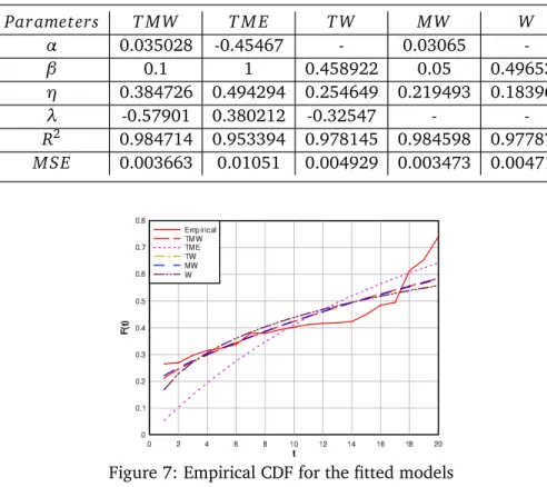
The analysis of least square estimates for the unknown parameters in these distributions namely: Transmuted Modified Weibull (TMW), Transmuted Weibull (TW), Transmuted Mod-ified exponential (TME), ModMod-ified Weibull (MW) and Weibull (W) distributions by using the method of least squares are defined. The LSE(s) of the unknown parameter(s), coefficient of determination(R2)and the corresponding Mean square error for transmuted modified Weibull families of distributions are given in Table 2.

We have provided the parametric estimate of the cumulative distribution function and the fitted functions in Figure 7. It is clear that the transmuted modified Weibull (TMW) distribution provides better fit than the other distributions. In this analysis some estimated values are negative which is not good in the LSE. Another check is to compare the respective coefficients of determination for these regression lines. We have supporting evidence that the coefficient of determination of (TMW) is 0.984714, which is higher than the coefficient of determination of (TME), (TW), (MW) and (W) distributions. Hence the data point from the transmuted modified Weibull (TMW) has better relationship and hence this distribution is good model for life time data.

Table 2: Estimated parameters of TMW, TME, TW, MW and W Distributions

Par ameters T M W T M E T W M W W

α 0.035028 -0.45467 - 0.03065

-β 0.1 1 0.458922 0.05 0.496531

η 0.384726 0.494294 0.254649 0.219493 0.183961

λ -0.57901 0.380212 -0.32547 -

-R2 0.984714 0.953394 0.978145 0.984598 0.977871 M SE 0.003663 0.01051 0.004929 0.003473 0.004713

9. Concluding Remarks

In this paper we introduce a new generalization of the Weibull distribution called trans-muted modified Weibull distribution and presented its theoretical properties. The new dis-tribution is very flexible model that approaches to different life time disdis-tributions when its parameters are changed. From the instantaneous failure rate analysis it is observed that it has increasing and decreasing failure rate pattern for life time data. This model has the capability to provide consistent results from all estimation methods.

References

[1] G. R. Aryall and C. P. Tsokos. Transmuted Weibull distribution: A Generalization of the Weibull Probability Distribution.European Journal of Pure and Applied Mathematics, Vol. 4, No. 2, 89-102. 2011.

[2] G. R. Aryall and C. P. Tsokos. On the transmuted extreme value distribution with ap-plications. Nonlinear Analysis: Theory, Methods and applications, Vol. 71, 1401-1407. 2009.

[3] R. Dumonceaux and C. Antle. Discrimination between the log-normal and the Weibull distributions,Technometrics, 15(4), 923-926. 1973.

[4] C.-C. Liu. A Comparison between the Weibull and Lognormal Models used to Analyze Reliability Data. PhD thesisUniversity of Nottingham, UK. 1997.

[5] G. Mudholkar, D. Srivastava, and G. Kollia. A generalization of the Weibull distribu-tion with applicadistribu-tion to the analysis of survival data.Journal of the American Statistical Association, 91(436):1575-1583, 1996.

[6] M. M. Nassar and F. H. Eissa. On the Exponentiated Weibull Distribution. Communica-tions in Statistics - Theory and Methods, 32(7):1317-1336, 2003.

[7] M. Pal, M. M. Ali, and J. Woo. On the exponentiated Weibull distribution. Statistica. (2):139-147, 2006.

[8] H. Pham and C.-D. Lai. On Recent Generalizations of the Weibull Distribution. IEEE Transactions on Reliability, 56(3):454-458, 2007.

[9] M. Z. Raqab. Inferences for generalized exponential distribution based on record Statis-tics.Journal of Statistical Planning and Inference. Vol. 104, 2, pp. 339-350. 2002.

[10] A. M. Sarhan and M. Zaindin. Modified Weibull distribution, Applied Sciences, Vol.11, 2009, pp. 123-136. 2009.

[12] W. Shaw and I. Buckley. The alchemy of probability distributions: beyond Gram-Charlier expansions and a skew-kurtotic-normal distribution from a rank transmutation map. Research report, 2007.

[13] M. Zaindin and A. M. Sarhan. Parameters Estimation of the Modified Weibull Distribu-tion,Applied Mathematical Sciences,Vol. 3, no. 11, 541-550. 2009.

Appendix

Proof of Theorem 2

µ_k=

Z ∞

0

tkf(α,β,η,λ,t)d t By substituting (2) into the above relation we have

µ_k=

Z ∞

0

tk(α+β ηtβ−1)exp(₋αt−ηtβ)(1₋λ+2λexp(₋αt−ηtβ))d t (A1)

Case A:In this caseα,β,η >0 and|λ| ≥1. The exponent quantity isE x p(−ηtβ)

E x p(−ηtβ) =

∞

X

i=0

(₋1)iηi(t)iβ

i! (A2)

Here equation (A1) takes the following form

µ_k=

∞

X

i=0

(₋1)i_ηi i!

(1₋λ)

_Γ(iβ+k+1)

αiβ+k +

β ηΓ(β(i+1) +k) αβ(i+1)+k

+2λ

∞

X

i=0

(₋1)i(2η)i

i!

_{αΓ(iβ+k+1)}

2αiβ+k+1 +

β ηΓ(β(i+1) +k)

2αβ(i+1)+k

(A3)

Case B:In this caseα=0,β,η >0 and_|λ_{| ≥}1.

µ_k=

Z ∞

0

tk(β ηtβ−1)exp(−ηtβ)(1−λ+2λexp(−ηtβ))d t

By substitutingw=ηt(β)then we get

µk=η −k

β _Γ

1+ k β



(1−λ) +λ2−

k β

‹

(A4)

Case C:In this caseα >0,β=0,η=0 and|λ| ≥1.

µ_k=

Z ∞

0

tkαexp(−αt)(1−λ+2λexp(−αt))d t

Proof of Theorem 3

M_x(t) =

Z ∞

0

et xf(α,β,η,λ,t)d t

By substituting (2) into the above relation we have

M_x(t) =

Z ∞

0

et x(α+β ηtβ−1)exp(−αt−ηtβ)(1−λ+2λexp(−αt−ηtβ))d t (A6)

Case A: In this caseα,β,η > 0 and _|λ_{| ≥} 1. The exponent quantity is E x p(₋ηtβ). Here equation (A6) takes the following form

Mx(t) = ∞

X

i=0

(−1)iηi

i!

–

(1−λ)

‚

αΓ(iβ+1) (α−t)iβ+1 +

β ηΓ(β(i+1)) (α₋t)β(i+1)

Ϊ

+2λ

∞

X

i=0

(₋1)i_(2η)i i!

–‚

αΓ(iβ+1) (2α−t)iβ+1 +

β ηΓ(β(i+1) +k) (2α−t)β(i+1)

Ϊ

(A7)

Case B:In this caseα=0,β,η >0 and_|λ_{| ≥}1.

M_x(t) =

Z ∞

0

et x(β ηtβ−1)exp(₋ηtβ)(1−λ+2λexp(₋ηtβ))d t

By substitutingw=ηt(β)then we get

M_x(t) =

∞

X

i=0

ti i!η

−k β _Γ

1+ i β



(1−λ) +λ2−

i β

‹