Extending the calibration of C IV-based single-epoch black hole mass estimators for active galactic nuclei

Park, et al. Published in Astrophyscial Journal, 839(2); 20 April, 2017 : 93-(1-21)

Extending

the

Calibration

of

C

IV-based

Single-epoch

Black

Hole

Mass

Estimators

for

Active

Galactic

Nuclei

DaeseongPark(박대성)1,2,3,10,AaronJ.Barth3,

Jong-HakWoo(우종학)4,MatthewA.Malkan5,TommasoTreu5,6,VardhaN.Bennert7,RobertoJ.Assef8,andAnnaPancoast9,11 1

KoreaAstronomyandSpaceScienceInstitute,Daejeon,34055,Korea; [email protected]

2

NationalAstronomicalObservatories,ChineseAcademyofSciences,Beijing100012,China

3

DepartmentofPhysicsandAstronomy,UniversityofCalifornia,Irvine,CA92697,USA; [email protected]

4

AstronomyProgram,DepartmentofPhysicsandAstronomy,SeoulNationalUniversity,Seoul,151-742,Korea; [email protected]

5

DepartmentofPhysicsandAstronomy,UniversityofCalifornia,LosAngeles,CA90095,USA; [email protected], [email protected]

6

DepartmentofPhysics,UniversityofCalifornia,SantaBarbara,CA93106,USA

7

PhysicsDepartment,CaliforniaPolytechnicStateUniversity,SanLuisObispo,CA93407,USA; [email protected]

8

NúcleodeAstronomíadelaFacultaddeIngeniería,UniversidadDiegoPortales,Av.EjércitoLibertador441,Santiago,Chile; [email protected]

9

Harvard-SmithsonianCenterforAstrophysics,60GardenStreet,Cambridge,MA02138,USA; [email protected]

Abstract

Weprovideanupdatedcalibrationof CIV l1549 broademissionline–basedsingle-epoch(SE)blackhole(BH) massestimators foractivegalacticnuclei(AGNs)usingnewdataforsixreverberation-mappedAGNsatredshift

6.5 7.5 41.7 43.8 −1_).

= 0.005 – 0.028with BH masses (bolometric luminosities) in the range 10 –10 M (10 –10 ergs

ew rest-frame UV-to-opticalspectra covering 1150–5700Åforthe six AGNs wereobtained with the Hubble Space Telescope (HST).Multicomponent spectraldecompositionsof the HST spectrawereused tomeasureSE emission-line widths for theCIV, MgII,andHβ lines,as wellas continuum luminositiesinthe spectralregion aroundeachline.Wecombinethenewdatawithsimilarmeasurementsforapreviousarchivalsampleof25AGNs toderivethemostconsistentandaccuratecalibrationsof theCIV-basedSE BHmassestimatorsagainsttheHβ reverberation-based masses,using three different measures of broad-line width: fullwidth at half maximum N

z

(FWHM), line dispersion(sline), and mean absolute deviation (MAD). Thenewly expandedsample at redshift

= 0.005 – 0.234 covers a dynamic range in BH mass (bolometric luminosity) of log M M☉ = 6.5 – 9.1

(

z

log L ergs−1 = 41.7 46.9), and derive the new CIV-based mass estimators using a Bayesian linear

BH –

regressio

bol

n analysis over this range. We ge we

nerallyrecommendtheuseofslineorMADratherthanFWHMtoobtain

alessbiasedvelocitymeasurementof theCIV emissionline,becauseitsnarrow-linecomponentcontribution is difficulttodecomposefromthebroad-lineprofile.

Keywords:galaxies: active– galaxies:nuclei–methods: statistical

1. Introduction BH estimators using the most reliable AGN BH mass

obtainedfromRMisthusimportantforimprovingthe estimates

mass

Understanding the cosmic growth of the supermassive black

precisionandaccuracyofSEmassestimatesforAGNs.Duetoa hole(BH)populationandthecoevolutionofBHswiththeirhost

lack of direct CIV RM measurements, however,CIV SE galaxiesis nowrecognizedtobeoneoftheessentialingredients

calibration has been performed against the Hβ RM-based BH for a complete picture of galaxy formation and evolution (see

masses, which is the best practical approach at present. Note Ferrarese&Ford2005andKormendy&Ho2013). To probe the

thatHβis,sofar,themoststudiedandunderstoodemissionline high-redshift BH populationand the evolution ofBH-galaxy

in RMstudies, with manyreliable Hβ-basedRM results;itcan scalingrelationsover cosmictime,itisessentialtohavereliable

thusbearguablyregardedasthemostreliablelineforAGNBH methodstodetermineBHmassesindistantactivegalacticnuclei

massmeasurements(seeShen2013forarelateddiscussion).

(AGNs;Shen2013).

Previously, Vestergaard & Peterson (2006, hereafter VP06) The rest-frame UV CIV l1549 broad emission line is

providedacalibration ofCIV-basedBHmassestimatorsusinga commonly used for BH mass estimates in high-redshift AGNs

sample oflow-redshift AGNsfor whichboth Hβ RMmeasure­

(i.e., 2  5) when single-epoch (SE) optical spectra are

mentsandrest-frameUVspectrawereavailable.Sincethen,the available. T

z

he method ofderiving SE mass estimates basedon

numberofAGNswithBHmassestimatesfromRMhasincreased, broad-line widths and continuum luminosities in quasar spectra

as has the number of AGNs for whichUV spectra have been relies onreverberation-mapped (RM)AGNsforits fundamental

obtainedbytheHubbleSpaceTelescope(HST). Park et al.(2013, calibration.12AchievinganaccuratecalibrationofCIV-basedSE

hereafter P13)revisited the calibrations of CIV-based BH mass estimatorsbytakingadvantageofhigh-qualityHSTUVspectrafor

*BasedonobservationsmadewiththeNASA/ESA Hubble Space Telescope,

theRMAGNsampleandusingimprovedmeasurementmethods.

obtainedat theSpaceTelescopeScienceInstitute,whichisoperatedbythe

Association ofUniversities forResearch in Astronomy, Inc., under NASA TheP13sampleincluded25AGNs,ofwhichsixhaveestimated

contract NAS 5-26555. These observations are associated with program _{M < 10} 7.5_M 7.0

andonlyonehasMBH< 10 M. In orderto

GO-12922. _imprBH_{ovethe calibrationofSE BHmasses atthe lowendofthe}

10

EACOAfellow.

11 AGN mass range (M_BH 107.5 M_), it is importantto further

NASAEinsteinfellow.

expand the sample of AGNs withboth RM measurements and 12

See a recent review by Bentz (2016) ofthe current status and future

basedonthebroadMgII l2798 emissionline,anothercommonly used rest-frame UV line atintermediate redshifts, has alsobeen performed(see,e.g.,McLure&Jarvis2002; Wang et al.2009). As with CIV, there is also much room for improvement in the calibration of MgII-based BH masses, and extending the calibration to a larger sample of AGNs over a wider dynamic rangeinBHmassisahighpriority.

Therehavebeenseveraleffortsintheliteraturetoimprovethe calibrationofCIV-basedSEBHmassestimators,e.g.,bytaking advantageof the ratio of UV to optical continuum luminosities

(color dependence; Assef et al. 2011), the ratio of fullwidth at half maximum (FWHM) to sline of CIV (line shape;

Denney2012),the peakfluxratioofthel1400 featureto CIV

(Eigenvector1;Runnoeetal.2013a;Brothertonetal.2015), and the CIV blueshift(Shen&Liu2012;Coatmanetal.2017).

Asanextensionofourpreviouswork(P13),thispaperpresents new HST UV and optical spectra of six RMAGNs with BH masses of 106.5_–107.5 _M

. High-quality spectra, quasi-simulta­

neouslycoveringtheCIV toHβspectralregionswithaconsistent aperture size and slit width, were obtained with the Space Telescope ImagingSpectrograph (STIS).The newdataenablea consistent comparison between the broad emission lines while minimizing measurement systematics due to time variability or apertureeffects.

Usingthenewspectra,weprovideupdatedcalibrationsofC IV-based SE BH mass estimators for three different measures of broad-linewidth:theFWHMandthelinedispersion(sline), which

have been commonly used in previous work on SE mass estimates, and the mean absolute deviation(MAD), which was recently suggested by Denney et al. (2016b) to be a useful linewidthmeasureforvirialmassestimation.

We use a Bayesian linear regression method, which is independently implemented for this work, to carry out the calibrationoftheCIV virialmassrelation.Ourmethodfollows thework ofKellyetal.(2012;seealsoKelly2007)usingthe

Stanprobabilisticprogramminglanguage(StanDevelopment Team2015a).TheBayesianmethodologyandmodelspecifica­ tions for the linear regression analysis will be described in detailinaforthcomingpaper(D.Park2017,inpreparation).

Thispaperisorganizedasfollows.InSection2,thecalibration sample, HST observations, and data reduction procedures are described. In Section 3, we present measurements of the CIV, MgII, and Hβ emission lines and comparisons oftheir profiles. ThenewcalibrationoftheSEvirialmassestimatorsbasedonthe FWHM,sline,andMADoftheCIV lineprofilearepresentedin

Section4withacomparisontopreviouscalibrationsandatestof methodological differencesin the linearregressionanalysis. We also systematically compare our updated calibration with the corrected prescriptions in the literature for the CIV BH mass calibrationdescribedabove.Wesummarizethisworkandprovide discussionin Section 5. The following standard cosmological parameters were adopted to calculate distances: H0=70

kms−1Mpc−1,W =m 0.30, andW =L 0.70, whichisthe same asusedbyP13.

2. Sample, HST Observations, and Data Reduction

Thesampleforthisworkisbasedonthesampleof25AGNs

(BH mass log MBH M =7.0 9.1, bolometric luminosity13 log Lbol

 –

ergs−1 =43.2 –46.9 , redshift z=0.009 – 0.234)

13_{ThebolometricluminosityiscomputedasL}

bol=3.81´lL1350(seeShen

etal. 2008andreferencestherein).

from P13, supplemented by six new AGNs at redshift

– thathavelow-massBHs(i.e.,

z=0.005 0.028 log MBH M=

6.5 – 7.5) from Hβ-basedRM measurements andlow bolometric luminosities(i.e., log Lbol ergs−1=41.7 – 43.8 ). TheP13sample

containsRMAGNswith availablearchivalHSTspectraselected by taking into account data quality, spectral coverage, and contamination of CIV by absorption features. The enlarged dynamic range in mass for the expanded sample enables us to calibratetheCIV SEvirialrelationshipoveralmostthreeordersof magnitudeinBHmass.Thenewtargetshavebeenselectedfrom recent RM programs. These include Arp 151, Mrk 1310, NGC 6814, and SBS 1116+583A from the Lick AGN Monitoring Project2008campaign(Bentzetal.2009b; Park et al.2012b), Mrk 50fromtheLickAGNMonitoringProject2011campaign(Barth etal.2011b), and theKepler-fieldAGNZw229-015(Barthetal. 2011a). Table1summarizesthepropertiesoftheP13AGNsample andthesixnewobjectspresentedinthiswork.Notethatthevirial factorfwithitsuncertaintyisadoptedfromParketal.(2012a)and Wooetal.(2010;seealsoWooetal.2013,2015)andappliedtoall RMBH masses (i.e., log f=0.71 0.31 ),which is consistent withpreviousmeasurementsanddirectmeasurementsbyPancoast etal.(2012,2014). Thefrepresentsthedimensionlessscalefactor oforderunitythatdepends onthedetailedgeometry,kinematics, andinclinationofthebroad-lineregion(BLR),whichisthusused to convert themeasured virial product into actual BHmass

(MBH = ´f VPBH). The adopted uncertainty (0.31dex) for the

virial factor is derived from the scatter of the AGN MBH -s_*

relation(0.43dex),whichgivesanupperlimitofrandomscatterof the virialfactor itselfafter subtractinginquadraturethe assumed intrinsic scatter (0.3dex) of the relation (see also the related discussion in Park et al. 2012b). Note that the virial factor uncertaintyisthedominantportionoftheerrorbudgetfortheRM masses, since the measurement uncertainty propagated from the reverberationlagsandHβlinewidthsissubstantiallysmallerthan this0.31dexuncertaintyforindividualAGNs(seeTable1).

For the six new AGNs, we obtained UV spectra with theSTIS as part of HST program GO-12922 (PI: Woo). In additiontothe UV data, optical spectrawereobtained quasi-simultaneously(during the same HST visit) with aconsistent slit width and aperture size. Note that thetemporal gaps between the end of the optical exposures and the start of theUV exposures were less than ∼6 minutes. Individual exposuresinandbetweenUVgratingswereobtainedwithina maximumtemporalgap of∼50minutes.Theabilitytoobtain nearly simultaneous UV and optical spectra through a consistent aperture is a unique capability of the STIS instrumentand is essential in order to minimize possible systematicbiasesfromAGNvariabilityand differentamounts ofhostgalaxyand narrow-lineregioncontributions.

Weusedthe G140L,G230L,and G430L gratingswiththe

Table1

OpticalSpectralPropertiesfromHβReverberationMapping

Object z tcent srms log(MBH/M) References

(Hβ) (Hβ) (RM)

(days) (kms−1)

(1) (2) (3) (4) (5) (6)

SamplePresentedin P13a

+1.1

3C120 0.03301 27.2-1.1 1514±65 7.80±0.31 6

+6.45

3C390.3 0.05610 23.60-6.45 3105±81 8.43±0.33 1

+4.57

Ark120 0.03230 39.05-4.57 1896±44 8.14±0.32 1

+3.75

Fairall9 0.04702 17.40-3.75 3787±197 8.38±0.32 1

+3.90

Mrk279 0.03045 16.70-3.90 1420±96 7.51±0.33 1

+1.21

Mrk290 0.02958 8.72-1.02 1609±47 7.36±0.32 4

+0.4

Mrk335 0.02578 14.1-0.4 1293±64 7.37±0.31 6

+5.75

Mrk509 0.03440 79.60-5.75 1276±28 8.12±0.31 1

+2.11

Mrk590 0.02638 24.23-2.11 1653±40 7.65±0.32 1

+2.45

Mrk817 0.03145 19.05-2.45 1636±57 7.66±0.32 1

+1.02

NGC3516 0.00884 11.68-1.53 1591±10 7.47±0.31 4

+2.80

NGC3783 0.00973 10.20-2.80 1753±141 7.44±0.32 1

+0.75

NGC4593 0.00900 3.73-0.75 1561±55 6.96±0.32 2

+0.86

NGC5548 0.01717 4.18-1.30 3900±266 7.80±0.34 3,5

+0.75

NGC7469 0.01632 4.50-0.75 1456±207 7.05±0.31 1

+26.20

PG0026+129 0.14200 111.00-26.20 1773±285 8.56±0.33 1

+24.30

PG0052+251 0.15500 89.80-24.30 1783±86 8.54±0.32 1

+18.85

PG0804+761 0.10000 146.90-18.85 1971±105 8.81±0.31 1

+22.10

PG0953+414 0.23410 150.10-22.10 1306±144 8.41±0.32 1

+79.70

PG1226+023 0.15830 306.80-79.70 1777±150 8.92±0.32 1

+21.45

PG1229+204 0.06301 37.80-21.45 1385±111 7.83±0.38 1

+41.30

PG1307+085 0.15500 105.60-41.30 1820±122 8.61±0.33 1

+33.50

PG1426+015 0.08647 95.00_-33.50 3442±308 9.08±0.34 1

+15.10

PG1613+658 0.12900 40.10-15.10 2547±342 8.42±0.38 1

+1.2

PG2130+099 0.06298 12.8-0.9 1825±65 7.63±0.31 6

NewSamplePresentedHere

+0.49

Arp151 0.02109 3.99-0.68 1295±37 6.83±0.32 3,5

+0.59

Mrk1310 0.01956 3.66-0.61 921±135 6.50±0.34 3,5

+0.82

Mrk50 0.02343 10.64-0.93 1740±101 7.50±0.32 7

+0.87

NGC6814 0.00521 6.64-0.90 1697±224 7.28±0.34 3,5

+0.62

SBS1116+583A 0.02787 2.31-0.49 1550±310 6.74±0.38 3,5

+0.69

Zw229-015 0.02788 3.86-0.90 1590±47 6.99±0.32 8

Note.Col.(1)Name.Col.(2)RedshiftsarefromtheNASA/IPACExtragalacticDatabase(NED).Col.(3)Rest-frameHβtimelagmeasurements.Col.(4)Line

2

dispersion(sline)measuredfromrmsspectra.Col.(5)TheMBHestimatesfromreverberationmapping:MBH(RM) =fVPBH=fctcentsrms G,wherethevirialfactor f

withitsuncertaintyisadoptedfromParketal.(2012a)andWooetal.(2010;i.e.,logf=0.710.31).Col.(6)References:1.Petersonetal.(2004);2.Denneyetal.

(2006);3.Bentzetal.(2009b);4.Denneyetal.(2010);5.Parketal.(2012b);6.Grieretal.(2012);7.Barthetal.(2011b);8.Barthetal.(2011a).

a

Notethatthesampleandmeasurementsarefrom P13.Onedifferencehereisthattheadopteduncertaintyforthevirialfactor(i.e.,0.31dex)hasbeenaddedin

quadraturetothefinalRMBHmassuncertainties,althoughthishomoscedasticuncertaintyadditiontothedependentvariablesdoesnotalteranyofthecalibration

resultsinthiswork,exceptforthevaluesofintrinsicscattertermandslightchangesintheconstraineduncertaintyrangesofregressioncoefficients.

Note thatthe slit positionangle (PA) wasnot constrained,in order tomaximize the HST scheduling opportunities. But the threegratingdataforeachobjectwereobtainedinasingleHST

visit withthesameorientation.

Whilewe used thefully reduced data providedbythe HST

STIS pipeline for the UV gratings, we performed a custom reductionfortheoptical gratingdatafromtherawscienceand reference files inorder toimprove the cleaning of cosmic-ray chargetransfertrailsintherawimagesfromthebadlydegraded STIS CCD. Based on the standard reduction of the STIS pipeline,anadditionalcosmic-rayremovalstepwasaddedtothe

processes employing the LA_COSMIC (van Dokkum 2001) routinefollowingtheapproachdescribedbyWalshetal.(2013). TherawdatafortheopticalG430Lgratingwerefirstcalibrated with the BASIC2D task, including trimming the overscan region,biasanddarksubtraction,andflat-fielding.Cosmicrays and hot pixels were then cleaned with LA_COSMIC, and wavelengthcalibrationwasperformed.

Table2

Summaryof HST/STISObservationsfortheSixNewAGNs

Observation

TotalExposureTime

Date SlitPA

G140L G230L G430L

(deg) (s) (s) (s)

Object

Arp151 2013Apr29 97.7 3801 2639 495

Mrk1310 2013Jun07 70.8 2624 1255 360

Mrk50 2012Dec12 −110.8 2624 1255 360

NGC6814 2013May07 −149.6 2848 1299 540

SBS 2013Jul12 28.9 3714 2648 600

1116

+583A

Zw229-015 2013Jul23 117.6 4302 2942 600

produceafinalsinglespectrumbytakingintoaccounttheflux and noise levels in overlapping regions around ∼1700and

∼3100Å.FollowingP13,wecorrectedthespectraforGalactic extinction using the values of E(B-V) from Schlafly & Finkbeiner (2011),as listedintheNASA/IPACExtragalactic Database (NED), and the reddening curve of Fitzpatrick

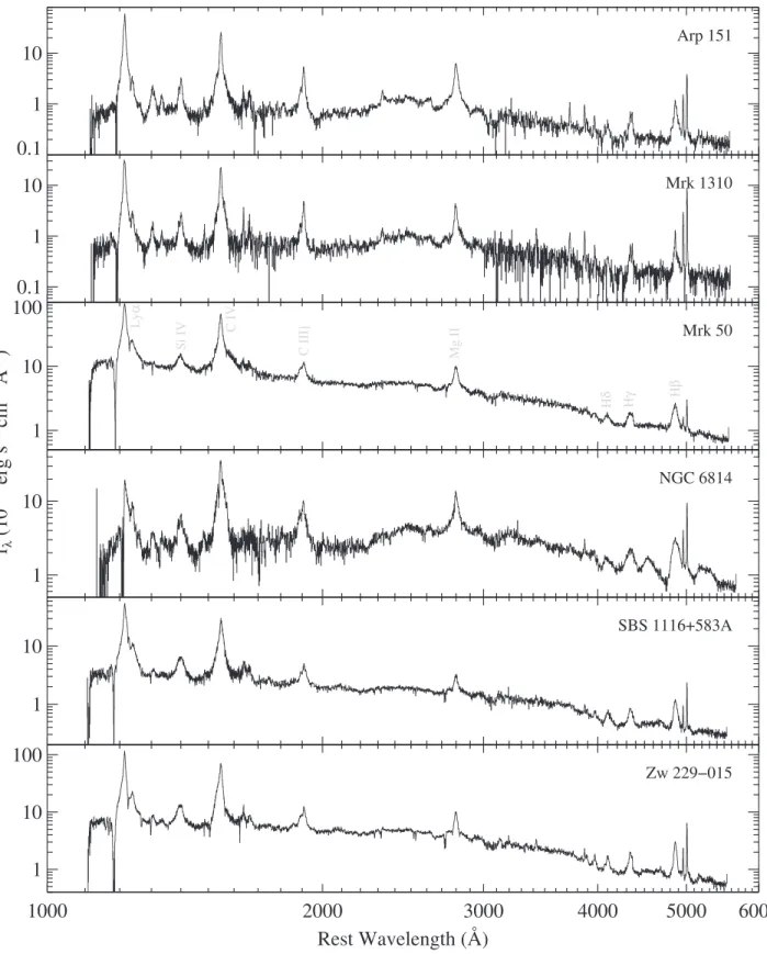
(1999).Figure 1 shows the fullyreduced and calibrated rest-frame spectraof thesixAGNs.

3. Spectral Measurements

To measure the broad emission-line widths and the continuum luminosity adjacent toeach broadline,we carried out a multicomponent spectral decomposition analysis ofthe spectralregionsurroundingCIV l1549, MgII l2798,and Hβ

l4861.Acombinationofthesetwoobservables,linewidthand continuum luminosity measured from anSEspectrum, is commonly used to estimate BH masses viaSE BH mass estimators because theycanbe adoptedas reasonableproxies for thevelocity of the broad-line gas clouds and the size of theBLR (Kaspi etal. 2000, 2005; Bentzet al. 2006, 2009a, 2013),respectively. Followingthestandard approach thathas beenadoptedinpreviousworks(e.g.,Shenetal.2008,2011), we measuredmonochromaticcontinuum luminositiesat1350, 3000,and5100ÅtocomputetheSEvirialmassesfromCIV, MgII,andHβ,respectively.

Our fitsare basedon alocaldecomposition of thespectral region around each broad line, rather than a global decom­ position of the entire UV-optical spectrum. Owing to the complexityofthespectraandthelargenumberofemission-line and continuum components that are present, we found that localdecompositions areabletoachieveamore precisefit to the data around each line than would be possible in a simultaneous,globalfittothefullSTISspectrum(seeSection 3.5 foradiscussion oftheglobal versuslocal fits). Thelocal spectral decomposition technique employed here is based on those byP13 and Park etal.(2015)and slightly updatedand modifiedfortheSTISdataandthespectralregioninquestion. Ourspectral-modelingmethod consistsofseparateprocedures for continuum fitting and line emission fittingapplied inde­ pendently to the CIV, MgII, and Hβ regions of the data. During fitting, model parameters are optimized using mpfit

(Markwardt 2009) in Interactive Data Language. The model components and fitting details for each of the Hβ, MgII,

andCIV line regions are described in the following subsec­ tions,and thedecompositionresults aregiven inFigure2.

3.1.Hβ

We used the multicomponent spectral decomposition code developedbyParketal.(2015)formodelingtheHβregionofour STISdata.Inbrief,thecodeworksbyfirstsimultaneouslyfittinga pseudocontinuum that consists of a single powerlaw, an FeII template,andahost-galaxytemplateinthesurroundingcontinuum regionsof4430–4770and 5080 – 5450 ÅandthenfittingtheHβ emissionlinecomplexwithGauss–Hermiteseriesfunctions(van der Marel&Franx 1993; Cappellari etal. 2002)for onebroad emissioncomponent(Hβ)andthreenarrowemissioncomponents

(Hβand[OIII]ll4959, 5007 )and two Gaussian functions for thenearbyblendedHeII l4686 emissionlineaftersubtractingthe best-fit pseudocontinuum model (see Park et al. 2015 and references thereinfor details of the measurement procedure;see alsoWooetal.2006;Bennertetal.2015; Runco et al.2016). The Hβlinewidths, FWHMHbandsHb,aremeasuredfromthebest-fit

broad-linemodel(i.e.,theGauss–Hermiteseriesfunction), andthe continuumluminosityat5100Å,lL5100Å,ismeasuredfromthe

best-fitpower-lawmodel.

Note that there are two differences between the method adopted here and the approach given by Park et al. (2015), specifically in the model components used for the FeII emission and host-galaxy starlight. The template for host-galaxy starlight is excluded in this work because stellar absorption features, which are critical to achievingreliable host-galaxy template fits, are not observable in the small-apertureSTISspectra.Theminimalcontributionofhost-galaxy light and the relatively low signal-to-noise ratio(S/N)and spectralresolutionoftheSTISopticaldatamakeitdifficultto detect any host-galaxy features. Moreover, the fits did not converge when we included the host-galaxy starlight comp­ onent in the model. As a rough check, we provided a crude estimateofanupperlimitforhost-galaxystarlightcontribution totheSTIS spectrausingthe objectSBS 1116+583A,which shows the highest host-galaxy fraction in the ground-based spectroscopic observations(seePark etal. 2012b;Barthetal. 2015)fromourSTISsample.Thehost-galaxyfluxintheSTIS spectrum can be roughly estimated by subtracting the AGN

flux at 5100Å, which is obtained by subtractingthe HST

imaging-basedgalaxyfluxat5100 Å(Bentzetal.2013)from the ground-based spectroscopic total flux at 5100 Å(Park et al. 2012b), from the total flux at 5100Å of the STIS spectrum. The resulting host-galaxy fraction in the STIS spectrumisfoundtobe∼31%.NotethattheotherAGNswill have much lower contributions due to the lower host-galaxy fractionsshownbyParketal.(2012b)andBarthetal.(2015). Available FeII templates for the Hβ region include empirically constructed monolithic templates by Boroson & Green (1992) and Véron-Cetty et al. (2004), a theoretical templatebyBruhweiler&Verner(2008),andasemi-empirical multicomponent template by Kovačević et al. (2010). After performing extensive tests using each of the templates and a linearcombinationofthemforourSTISdata,weoptedtouse the template ofKovačević et al. (2010) based on its overall performanceas quantifiedbythec2_{-statisticsand residualsof}

Figure1.FinalfullyreducedandcombinedSTISspectraforoursampleofthesixlow-massAGNs.

strong FeII emission. The Kovačević et al. (2010) template emission, and we omitted the host-galaxy starlight template appearstobethebestcurrentlyavailableforaccurately fitting fromthe fits.

diverseFeII emissionblendsinAGNsbyallowingfordifferent relative intensities between five FeII multiplet subgroups. To

3.2.MgII

sum up, we followed the method described by Park et al.

(2015), exceptthat we used the template of Kovačevićet al. FortheMgII spectralregion,wefirstfitapseudocontinuum

Figure2.Multicomponentspectraldecompositionsinthespectralregionsofthreemajorbroademissionlines—CIV l1549, MgII l2798,andHβ l4861—forour

sixAGNs.Ineachpanel,theobservedspectrum(black)isdecomposedintovariouscomponents.Leftpanels(CIV):power-lawcontinuum(green), CIV l1549

(magenta), and other nearby blendedlines, includingNIV]l1486 (orange), HeII l1640 (blue),andOIII]l1663(brown).Middle panels (MgII):power-law

continuum(green), FeIItemplate(orange),Balmercontinuum(blue),andMgII l2798(magenta).Rightpanels(Hβ):power-lawcontinuum(green), FeIItemplate

(orange),threenarrowemissionlines (Hβand[OIII] ll4959,5007blue),broadHβ(magenta),andbroadandnarrowHeIIl4686components (brown;only

includedifblendedwithHβ).Theredlinesineachpanelindicatethefullmodelcombiningallthebest-fitmodelcomponents.Thegraylinesatthebottomofeach

2850–3100Å.The pseudocontinuummodeliscomposed ofa single power-law function representing the AGN featureless continuum,anFeII emissiontemplate,andanempiricalmodel fortheBalmercontinuum. WeadoptedtheUVFeII template, whichismadefromobservationsofIZw1,fromTsuzukietal.

(2006).UsingthetemplateofTsuzukietal.(2006)isarguably better for modeling the MgII line region than using that of Vestergaard & Wilkes (2001)because it contains semi-empiricallyconstrainedFeII contributionunderneaththeMgII line,whilethetemplatebyVestergaard&Wilkes(2001)hasno FeII flux at all under the MgII line due to the difficulty of decomposing thisspectralregion.

BasedontheinvestigationsofGrandi(1982)andWillsetal.

(1985; seealsoMalkan &Sargent 1982for thefirstpractical measurement of theBalmer continuum shape), Dietrichet al.

(2002, 2003) described a practical procedure forBalmer continuum modelinginhigh-zquasarspectrathathasbecome a standard practice for fitting the Balmer continuum. This empirical model assumes that the Balmer continuum is generated from partially optically thick gas clouds with auniformeffective temperature(Te= 15, 000 K )as

BaC -tBE (l lBE )

F_l (A T, e,tBE)=ABl( )(Te 1 -e

3

) , l  lBE, ( )1

where A and tBE are thenormalized flux density and optical

depth at the Balmer edge (lBE = 3646 Å), respectively,and

Bl( )Te isthePlanckfunctionattheelectrontemperatureTe. At l>lBE,higher-orderBalmerlinesusingtherelativeintensity

calculations from Storey & Hummer (1995) are used to represent the smooth rise to the Balmer edge. Many studies

(e.g., Kurketal.2007;Wang etal.2009;Greeneetal.2010; De Rosaetal.2011,2014;Hoetal. 2012;Shen&Liu2012; Kokubo et al. 2014) have used variants of this method with slightly different ways of constraining the model parameter ranges based on the available data quality and spectral coverage. Wefound thatif wetreated allthree parametersin the model (A,Te,tBE) as free parameters during fitting, as

wasdonebyWangetal. (2009)andShen&Liu(2012),they were very poorlyconstrained due tothe degeneracy with the power-law continuumand FeII emissionblends.

Recently, Kovačević et al. (2014) suggested an improved way toconstrain the normalization A:by taking into account thefact that A can be obtained by calculatingthe sum of all intensitiesofhigher-orderBalmerlinesattheBalmeredge.We followedthisprocedurewithslightmodifications.Thevalueof

A was separately determined from the intensity calculation usinghigh-orderBalmerlines(upto400)withthetemplateline profile adopted from the best-fit Hβ emission-line model obtained above. The other parameters, Te andtBE, werethen fitted simultaneously with the FeII template and power-law function during pseudocontinuum modeling. However, it should be notedthat,following the Dietrich approach, the temperature was finallyfixed tobe 15,000K, and theoptical depth was allowed to vary between 0.1 and 2. We also independentlycheckedthattheconstrainedBalmercontinuum componentonlyexhibitedmarginalchangesovertemperatures ranging from 10,000to 30,000K and optical depths varying from 0.1 to 2. Note that the resulting continuum luminosity estimates are consistent with each other within ∼0.04dex scatter.

After subtracting the best-fit pseudocontinuum model, the MgII emissionlinewas fittedusingalinear combinationofa

sixth-order Gauss–Hermite series and a single Gaussian function toaccount for itsfull lineprofile, typicallyshowing amore peaky core (i.e.,narrower and sharper linepeak) and more extended wings thana Gaussian profile, in the spectral region ∼2700–2900Å. We usethe full lineprofile without a decomposition of narrow and broad components for theline width measurements for UV lines in this work (the same approach adoptedbyP13),incontrasttoHβ.This isbecause no reliable and clear distinction between broad and narrow componentsintheUVlinesisusuallypossible,andsometimes no narrow components of the UV lines are seen at all;their presenceisstilluncertainandunderdebate.Thus,theMgII line widths, FWHMMgII andsMgII, are measuredfrom thebest-fit

fulllineprofile,andcontinuumluminosityat3000Å,lL3000Å,

is measured from the best-fit power-law function. During

fitting, Galactic absorption lines such as FeII ll2586, 2600 , MgII ll2796, 2803,andMgI l2852 (cf.Savaglioetal.2004) aremaskedoutwithexclusionwindows.

3.3. CIV

Spectralmeasurements for theCIV lineregioninthearch­ ivalsampleofthelocal25RMAGNsweredescribedbyP13. Here, we focus on analysis of the sixobjects with newly obtainedSTISdata. Weusedthesame methodsasinP13for consistency and to avoid additional systematic biases. Wefit the AGN featureless continuum with a single power-law function, and we chose to omit a UV iron template (e.g., Vestergaard & Wilkes 2001) from the fits because no clear contribution of iron emission over the CIV region wasob­ served.AlthoughweperformedatestbyincludingtheUViron templateinthemodelasinP13,itscontributionwastoosmall tobeconstrained accurately with thetemplate, atleast inour sample(seealsoShenetal. 2008,2011).

Afterthebest-fitcontinuummodelwassubtracted, theCIV emissionline wasfittedwith alinear combination of a sixth-order Gauss–Hermite series and a single Gaussian function. The contaminatingnearby blendedemission lines(e.g., NIV]

l1486, SiII l1531, HeII l1640, andOIII]l1663) werefitted simultaneouslyaswellusinguptotwoGaussianfunctionsfor eachline.Again,weusedthecombinedmodelofone Gauss– Hermitefunctionandone Gaussianfunctiontofitthefullline profileofCIV without decomposingit intobroadand narrow components.TheCIV linewidths,FWHMCIVandσCIV,were measured from the best-fit full line profile, and continuum luminosityat1350Å,lL1350Å,wasmeasuredfromthebest-fit

power-law function. Narrow absorption spikes were masked out using a 3s clipping threshold during fitting, and broad absorption features around the line center were masked out manually with exclusion windows (see P13 and references thereinfor moredetails of the CIV measurementmethod and resultsforthearchival sample).

3.4.MeasurementUncertaintyEstimation

Uncertainties for the above spectral measurements are estimated with the Monte Carlo method used by Park et al.

Table3

UltravioletSpectralPropertiesfromCIVSEEstimates

Object Telescope/Instrument Date Observed S/N

(1450 or 1700 Å)

(pix−1)

E B( -V)

(mag)

L log( ll erg s−1₎

(1350 Å)

FWHMSE

(C IV) (km s−1)

sSE

(C IV) (km s−1)

MADSE

(C IV) (km s−1)

W X,

r( ) r( W Y, ) r( W Z,

(1_{) (}2_{) (}3_{) (}4_{) (}5_{) (}6_{) (}7_{) (}8_{) (}9_{) (}10_{) (}11_{) (}12₎

Sample Presented in P13a

3C 120 3C 390.3 Ark 120 Fairall 9 Mrk 279 Mrk 290 Mrk 335 Mrk 509 Mrk 590 Mrk 817 NGC 3516 NGC 3783 NGC 4593 NGC 5548 NGC 7469 PG 0026+129 PG 0052+251 PG 0804+761 PG 0953+414 PG 1226₊023 PG 1229+204 PG 1307+085 PG 1426+015 PG 1613+658 PG 2130+099

IUE/SWP

HST/FOS

HST_/FOS

HST_/FOS

HST/COS

HST/COS

HST/COS

HST/COS

IUE_/SWP

HST/COS

HST/COS

HST/COS

HST/STIS

HST_/COS

HST_/COS

HST/FOS

HST/FOS

HST/COS

HST/FOS

HST_/FOS

IUE/SWP

HST/FOS

IUE/SWP

HST/COS

HST/COS

1994 Feb 19,27;1994 Mar 11 1996 Mar 31

1995 Jul 29 1993 Jan 22 2011 Jun 27 2009 Oct 28

2009 Oct 31;2010 Feb 08 2009 Dec 10,11 1991 Jan 14

2009 Aug 04;2009 Dec 28 2010 Oct 04;2011 Jan 22 2011 May 26

2002 Jun 23,24 2011 Jun 16,_17 2010 Oct 16 1994 Nov 27 1993 Jul 22 2010 Jun 12 1991 Jun 18 1991 Jan 14,_15 1982 May 01,02 1993 Jul 21 1985 Mar 01,02 2010 Apr 08,09,10 2010 Oct 28

12 18 17 24 9 24 29 107 17 38 20 29 10 36 32 25 21 34 18 93 28 14 45 37 22 0.263 0.063 0.114 0.023 0.014 0.014 0.032 0.051 0.033 0.006 0.038 0.105 0.022 0.018 0.061 0.063 0.042 0.031 0.012 0.018 0.024 0.030 0.028 0.023 0.039

44.399±0.021 43.869±0.003 44.400_±0.005 44.442±0.004 43.082±0.004 43.611±0.002 43.953±0.001 44.675±0.001 44.094_±0.007 44.326±0.001 42.615±0.002 43.400±0.001 43.761±0.005 43.822_±0.001 43.909_±0.001 45.236±0.005 45.292±0.004 45.493±0.001 45.629±0.005 46.309_±0.001 44.609±0.009 45.113±0.006 45.263±0.004 45.488±0.001 44.447_±0.001

3093±291 5645±202 3471_±108 2649±77 4093±388 2052±36 1772±14 3872±18 5362_±266 4580±48 2658±34 2656±444 2952±166 1785_±82 2725_±66 1604±50 5380±87 3429±23 3021±74 3609_±29 4023±163 3604±111 4220±258 6398±51 2147_±18

3106±157 6154±65 3219_±53 2694±20 2973±53 3531±32 1876±12 3568±9 3479±165 3692±23 4006±49 2774±91 2946±162 4772_±80 2849±237 4965±113 4648±50 2585±20 3448±55 3513_±29 2621±90 4237±80 4808±305 4204±17 2225_±47

2280±74 4674±42 2345_±31 1987±13 2202±18 2544±14 1311±7 2601±6 2630±139 2756±14 2864±29 2014±9 2135±33 3528_±102 2060±15 3610±77 3463±30 1932±13 2472±35 2595_±19 1989±62 3010±54 3549±95 3286±13 1554_±21

−0.05 −0.11 0.01 0.04 0.01 −0.00 0.03 0.02 −0.09 −0.01 −0.03 −0.01 −0.01 0.02 −0.02 −0.04 −0.12 0.04 −0.02 −0.18 −0.29 −0.13 −0.10 −0.01 0.02 −0.35 −0.30 −0.30 −0.21 −0.04 −0.13 −0.02 −0.07 −0.12 −0.25 0.07 −0.01 −0.00 −0.11 −0.01 −0.11 −0.54 0.14 −0.43 −0.52 −0.48 −0.57 −0.23 −0.10 −0.06 −0.50 −0.32 −0.37 −0.17 −0.11 −0.20 0.02 −0.03 −0.05 −0.21 0.06 −0.17 −0.02 −0.02 −0.14 −0.22 −0.61 0.17 −0.48 −0.60 −0.49 −0.58 −0.42 −0.04 −0.07

New Sample Presented Here

Arp 151 Mrk 1310 Mrk 50 NGC 6814 SBS 1116+583A Zw 229-015

HST/STIS

HST/STIS

HST/STIS

HST/STIS

HST/STIS

HST_/STIS

2013 Apr 29 2013 Jun 07 2012 Dec 12 2013 May 07 2013 Jul 12 2013 Jul 23

6 5 19 6 13 17 0.012 0.027 0.015 0.164 0.010 0.064

41.791±0.017 41.715±0.025 43.213±0.003 41.105±0.021 42.867±0.005 43.129_±0.007

1489±26 1434±78 2807±63 2651±264 3253±302 2573_±71

2900±61 2447±108 4443±160 2804±103 3315±231 2608_±56

1864±35 1603±54 3140±115 2096±59 2302±121 1891_±33

−0.03 0.00 0.02 0.02 −0.04 −0.05 −0.38 −0.25 −0.13 −0.07 −0.13 −0.20 −0.46 −0.31 −0.10 −0.11 −0.15 −0.18

Note.Col.(1)Name.Col.(2)Telescope/instrumentfromwhicharchivalUVspectrawereobtained.NotethatthenewCOSspectrawereobtainedafter2009.Col.(3)Observationdateforcombinedspectra.Col.(4) S/Nperpixelat1450or1700Åintherestframe.Col.(5)Valueof E(B-V)fromtheNEDbasedontherecalibrationofSchlafly&Finkbeiner(2011).Col.(6)Continuumluminositymeasuredat1350Å.Col.(7) FWHMmeasuredfromSEspectra.Col.(8)Linedispersion(sline)measuredfromSEspectra.Col.(9)MAD(meanabsolutedeviationaroundweightedmedian)measuredfromSEspectra.Col.(10)Correlation

coefficientbetweenmeasurementerrorsof W and X,where W=loglLl at1350Åand X=logFWHMSE.Col.(11)Correlationcoefficientbetweenmeasurementerrorsof W and Y,where Y=logsSE.Col.(12)

Correlationcoefficientbetweenmeasurementerrorsof W and Z,where Z=logMADSE. a

thestandard deviationofthedistributionofthemeasurements as theestimateofthemeasurementuncertainty.

Typical uncertainty levels of line widths for all objects are found to be∼2%–4%withamaximumof∼17%duetothehigh qualityoftheHSTspectra.Forcontinuumluminosity,wederive uncertaintiesof ∼1%–2% with amaximumof ∼6%.These are smallcomparedtotheoverallsystematicmassuncertaintyof∼0.4 dexin the SEvirialmethod. Covariances betweenthemeasure­ ment uncertainties of the line widths and luminositiesfor each objectinalogarithmicscalearealsoestimatedfromtheresulting distributions of the Monte Carlo simulations, which are given as cov ( log lLl, logFWHM )=rs(log lLl) (s logFWHM ) and

cov (log lLl, log sline)=rs(log lLl) (s log sline),where cov,ρ,

andσarethecovariance,correlationcoefficient,andmeasurement uncertaintyofthelogarithmsoftheluminositiesandlinewidths, respectively.Table3liststhelinewidthsandluminositiesforour sample,alongwiththemeasurementuncertaintiesandtheirerror correlationcoefficients.

3.5.ContinuumLuminositiesandEmission-Line Widths

There areseveral issues inregard tomeasuring continuum luminosities andlinewidths accurately.Itisimportanttotake intoaccounttheBalmercontinuumovertheMgII lineregionin orderto accurately decompose the power-law continuum for theluminositymeasurements.Basedonourinvestigationofthe STIS data, the lL3000Å values willbe overestimated by ∼0.14dex,on average, if the Balmer continuum component is not accounted for.Thisisconsistent with the investigation of Shen & Liu (2012), who found a∼0.12dex systematic offset. This bias will then be propagated into the final MBH

estimatesbyasmuchasa∼0.07dex(∼17%)systematicoffset iftheBalmer continuummodelisnotincludedproperly.

IftheoriginalVestergaard&Wilkes(2001)FeII templateis used,theFWHM (sline)estimatesareoverestimatedby∼0.03 (0.07)dex,onaverage,comparedwiththeresultsderivedusing the template of Tsuzuki et al. (2006). This will again be propagatedintotheMBHestimatesbyupto∼0.06(0.14)dexof

systematicoffset,whichisconsistentwiththeresultofNobuta etal.(2012).

Tomakethemaximumuseofthewidespectralcoverageofour STISdata,wealsoperformedextensivetestsofglobalcontinuum

fits coveringCIV to Hβ simultaneously. Using amore flexible double power-law model to represent the AGN featureless continuum, we fit a pseudocontinuum model including the Balmer continuum model and FeII emission to many line-free continuum regions(see also,e.g., Shen&Liu2012and Mejía-Restrepo et al. 2016 for related recent work). The global continuum fits produced results consistent with the local continuumfitsdescribedintheprevioussections,exceptthatthe globalfitsfailedtoconstraintheFeII emissionontheredsideof the MgII regionsfor Arp 151and Mrk1310. This is probably because the double power-law model is not flexibleenough to properly describethesteeplocal slope changesaroundMgII for these two objectsthat are coming from intrinsic changes of spectralshapesand/orfromstronginternalreddening,alongwith the incompleteness of currently available UV FeII templates across the regions. In any case, there is no significant improvementofthe globalfitscomparedtothelocalfits.

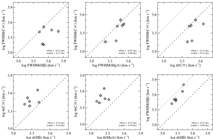
The simultaneous coverage of ourSTIS dataalsomakes it possible to consistently compare the major UV and optical emission lines (CIV, MgII, andHβ) without biases from intrinsic variability (Figure 3). The CIV profile shows, on

average,morepeaky coreswithextendedwingsthanthoseof theMgII andHβ lines(seealsoWillsetal.1993;Brotherton etal.1994).Thereisnosignificantvelocityoffsetbetweenthe line peaks ofthe three emission lines. Figure 4 compares FWHMandslinelinewidthmeasurementsamongtheemission

lines.Althoughitishardtodrawaclearpicturedueto small-numberstatistics,weuseonlyourSTISsampleofsixAGNsin order to perform a consistent comparison between the line widthsinquasi-simultaneouslyobserveddata.Wefindthatthe FWHM of CIV is, on average, smaller than that ofHβ (and MgII), which may indicate that theFWHM ofCIV is not a good proxy for virial BLR velocity, probably due to contamination from a nonreverberating CIV core component

(Denney2012).Thiscontaminationwouldbeoneofthebiases correlatedwithEigenvector1 (EV1;Boroson&Green1992), as discussed by Runnoe et al. (2013a, 2014) and Brotherton etal.(2015).Theyinvestigatedandusedthepeakfluxratioof thel1400 featuretoCIVasaUVindicatorofEV1tocorrect for theCIV-basedBH masses.However, the interpretation is not straightforward. It could also be the case that the BLR geometryisdifferentfortheregionsemittingthesethreelines, resultingindifferentindividualvirial factors(f)foreachline

(see also Runnoe et al. 2013b). By contrast, σC IV is, on average,larger thansHb, which is consistent with the simple

virial expectation of stratified BLR structure and the shorter reverberation lags of CIV (Peterson & Wandel 1999; Kollatschny 2003), thus corroborating the use of sline over

FWHM for CIV-based BH mass estimates. More detailed intercomparisons and systematic investigation of multiline properties including more objects from the literature will be presentedinaforthcomingpaper.

4. Bayesian Calibration of C IV-Based MBH Estimators

Nowthatwehavethecontinuumluminosity andlinewidth measurements from the SEspectra, we can perform a calibration of the CIV-based SE BH mass estimators against the Hβ RM-based BH masses as afiducial baseline. We assume that the BH masses from theHβ RM are the most reliable mass estimates available for these galaxies, and our goalistofindthecombinationofSEmeasurements thatmost closely reproduces the RM mass scaleusing the following equation:

⎛ RM⎞ ⎛ l_LSE ⎞

M_{BH 1350.Å}

log =a + b log

⎝ ⎜

⎠ ⎟

⎝

⎜ _{44 -1} ⎠ ⎟

M 10 erg s

⎛ DVSE ⎞

g log

⎝

⎜ CIV

-1_⎠⎟, ( )

+ 2

1000 km s

SE SE SE

whereDV_CIV= FWHMCIV orsCIV.This equationessentially

expressesthevirial relation MBH ~rBLRV2 G,assumingthat

theBLR radius scales with AGN luminosity according to

rBLRµLbandallowingforthevirialexponentγtodifferfrom

the physically expected value of 2 in order to achieve the bestfit.

Figure3.Comparisonofthemodeledemission-lineprofiles,normalizedbyeachpeak,ofCIV(red), MgII(green),andHβ(black)forourSTISsample.

2014;see also Shen et al. 2016b), most of the available reverberationstudieshave beendonewiththeHβ line,which gives themostreliableAGNBHmassesatpresent.

Toperformthecalibration,weadoptaBayesianapproachto linear regression analysis. An advantage of the Bayesian method over the traditional c2_{-based methodis that, by}

obtaining probabilitydensity functions(PDFs) forparameters of interest instead of just calculating a point estimate, it provides morereliable uncertainty estimates,incorporatingall the error sources modeled and simply marginalizing over nuisance parameters. Itis alsoeasy toexplore thecovariance between parameters from resulting joint probability distribu­ tions. The Bayesian linear regression method outperforms otherclassicalmethods,especiallywhenthemeasurementerror oftheindependentvariablesislargeand/orthesamplesizeis small(seeKelly2007).

ForthefullBayesian inference,weusetheStan probabil­ istic programminglanguage(StanDevelopmentTeam2015a), which contains an adaptiveHamiltonian MonteCarlo(HMC; Neal2012; Betancourt&Girolami 2013)No-U-Turnsampler

(NUTS;Hoffman&Gelman2014)asitssamplingengine.This provides a simple implementation for specifying complex hierarchicalBayesianmodelsandachievesgoodcomputational efficiency. We set up the Bayesian hierarchical model followingKellyetal.(2012)andimplement itbyreferringto Gelman et al. (2013), Kruschke (2014), and theStan Devel­ opmentTeam(2015b).Thepracticaldetailsofthesamplerand the model specification will be described ina separate paper discussingthemethodology (Park2017,inpreparation). As a brief summary, the t-distribution is adopted to obtain anoutlier-robust statistical inference following the invest­ igationofKellyetal.(2012),withanadditionalimprovement of treating degreesoffreedom in the t model as a free parameter, instead of fixing it to be a preselected constant. Thus, the likelihood function, whichspecifiesthe measure­ ment, regression, and covariate distribution models, is built witht-distributions, and the prior distributions are specified based onsuggestions byBarnard etal. (2000), Gelmanet al.

(2013),andKruschke(2014).OurMarkovchainMonteCarlo

(MCMC)simulationshavebeenrunviathePyStanpackage

(v2.9.0; Stan Development Team 2016) with careful assess­ mentof theconvergenceoftheMCMCchains.

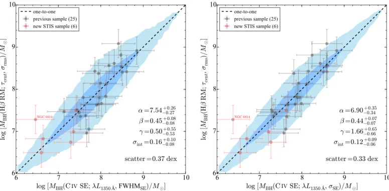
4.1. TheSEMass Calibration

Figure5 shows the results of the calibration of CIV-based SEBHmassestimatorsagainsttheHβ-basedRMmassesusing thefullsampleof31localRMAGNswithEquation(2),while Figure 6 presents thecorresponding marginal projections of each pair of parameters of interest with one-dimensional marginalized distributionsfrom thefull posterior distribution, fromwhich parametercovariancesaresimplyidentifiable.We takethe best-fitvalues and uncertainties of the parametersof interest(a b g, , , andsint)fromposteriormedianestimatesand

68% posterior credible intervals, as recommended by Kelly

(2007)and Hoggetal.(2010).

IneachpanelofFigure5,thetwomassestimates(RMand SE) are fairly consistent. The overall scatter of the SE BH massesbasedonthecalibratedequationusingtheCIV FWHM

(sline) compared to the RM BH masses are at the level of

0.37dex (0.33dex). This indicatesgenerallyquite good con­ sistency, given theunavoidable object-to-object scatter of the virial factor f (0.31dex; Woo et al. 2010), since we are adoptingasingleensembleaveragevalueoftheffactorforall objects.

Toassesstheresultingmodelfittothedata, wepresentthe posteriorpredictivedistribution(blueshadedcontour),whichis generated fromsimulations according tothe fit parametersof themodel,tocheckwhethertheposteriorpredictionreplicates theoriginalobserveddatadistributionreasonablywell.Ascan be seen, the 95% credible region depicted by the light blue shadedcontour describes most of the data distribution well, except for one outlier:NGC 6814. We have also calculated posterior predictive p-values by following the method of Chevallard&Charlot(2016;seealsoGelmanetal. 2013and

2

thePyMCUser’sGuide14).Usingc devianceasadiscrepancy

14

⎞ ⎠ ⎛

⎝ ⎤ ⎦ ⎡

⎣

Figure4.Intercomparisonoflinewidthmeasurements,FWHMand sline, ofCIV, MgII,andHβforourSTISsample.Thedashedlineineachpanelrepresentsaone­

to-onerelation.ThedottedlinesshowtheratioofFWHMto slineforaGaussianprofile.Themeanoffset(i.e.,averageoflinewidthdifferences)and1σscatter(i.e.,

standarddeviationoflinewidthdifferences)aregiveninthelowerrightcornerofeachpanel.

measure, the Bayesian p-value estimates are mostly ∼0.2, affectedbyacontaminatingnonvariableCIV corecomponent ranging from 0.14 to0.26 inthis work, indicating successful (seealsoP13andDenneyetal.2013forrelateddiscussionand modelfitstothedata.Notethatthereisaproblem(e.g.,misfit interpretation).Velocityslopes that areshallower (0.50, 1.66) or inadequacy in the descriptive model) if the p-value is thanthevirial expectation(2)would alsobe expectedinpart extreme, i.e., <0.05 or >0.95. All the calibration results due toan additional dispersion of the measured line-of-sight performed inthiswork forvariouscasesarelistedinTable4. velocitiesstemming fromorientationdependence(seeShen& Notethat thepresenceofthesingle outlier,which isnotvery Ho2014).

extreme,doesnotalteranyoftheconclusions,andvirtuallythe Ourfinalbestfitsareasfollows(seealsoTable4):

⎜ ⎟

⎢ ⎥

⎤ ⎦ ⎡

⎣

⎢ ⎥

FWHM-basedandsline-basedestimators.Thismayalsoimply + 2 log

sameresultisobtainedforthegivenuncertaintiesiftheoutlier

l

MBH(SE) L1350Å

isremoved. +0.07

6.73 0.43 +0.06

log = -0.07 + -0.06 log

1044_{erg s} 1

M

-Theluminosity slope,β,isconsistentwiththephotoioniza­

tion expectation (i.e., 0.5) within theuncertainties for both _{s(C IV)}

, -1 1000 km s

thatthesize–luminosityrelationfortheUV1350Åcontinuum

3 ( )

hasaslopeconsistent withthe relationfortheoptical5100Å

+0.035

continuum(e.g., 0.533 -0.033byBentzetal.2013).Thevelocity

⎞ ⎠ ⎛

⎝ ⎤

⎦ ⎡

⎣

withtheoverallscatteragainstRMmassesof0.33dex,which

RM

⎢ ⎥ ⎜ ⎟

slope, γ, for the sline-based estimator is close to the virial _{is de}fi_{ned by the}_{standard deviation of mass residuals}

expectation (i.e., 2)within theuncertainties, while thisis not the case for the FWHM-based estimator, whose γ value is consistent with zero, given the uncertainty interval. This is generally consistent with the calibration resultbased on CIV

( ) BH(SE)

D = log MBH -logM ,and

l

MBH(SE) +0.26 L1350Å 0.45 +0.08

log =7.54 -0.27 + -0.08 log

1044_{erg s} 1

M

-FWHM by Shen & Liu (2012), who found a much smaller

FWHM (C IV) -1000 km s 1 ,

slope (0.242)than2,althoughtheirluminositydynamicrange probedismuchhigherthanours.Andthesline-basedSEmasses

+0.55

+ 0.50 -0.53log

⎤ ⎦ ⎡

⎣⎢ ⎥

show overall less intrinsic and total scatter thanthe FWHM- _{( )}

based masses. Thus, this indicates that the CIV σ is abetter

withtheoverallscatteragainstRMmassesof0.37dex.Forthe traceroftheBLRvelocityfieldthantheCIV FWHMbecauseit

is closer to the virial relation and shows less scatter inmass caseofthesline-basedestimator,notethatthevalueofγisfixed

estimates. Theseresultsareinoverallagreement withthoseof at 2 (i.e., consistent with the virial expectation) in our final Denney(2012),whofoundthattheCIV FWHMismuchmore analysis because it is consistent with 2 within theuncertainty

Figure5.CalibrationresultsofCIV-basedSEBHmassestimatorsusingFWHM(left)and sline(right).Thenewlyaddedlow-massAGNsample(sixobjects)is

indicatedwithredcircles,whiletheblackcirclesrepresentthepreviousarchivalsampleof25objectsfrom P13.Blueshadedcontours,whosedarkblue(lightblue)

areacorrespondstothe68%(95%)credibleregion,showtheposteriorpredictivedistributionsunderthefittedmodelasaself-consistencycheck(seetext).The

resultingregressionparameterswiththeuncertaintyestimatesandoverallscatteraregiveninthelowerrightcornerofeachpanel.Notethattheerrorbarsinthe y-axis

(RMmass)representthequadraticsumofthepropagatedRMmeasurementuncertaintyforthevirialproduct(VP)andtheadopteduncertaintyforthevirialfactor,and

thoseinthe x-axis(SEmass)representthequadraticsumofthepropagatedSEcalibrationuncertaintyandtheresultingoverallscatter.

estimate when we treat it as afree parameter. Fixing γtothe physically motivated value helps to avoid possible object-by­ objectbiasesandsystematicsduetosmall-numberstatisticsand reduces the uncertainties of the other resulting regression parameters (seealsoP13).Theoverallscatterofthesline-based

calibrationisvirtuallyunchangedifwefixg= 2,whilethatof theFWHM-basedcalibrationincreasesconsiderablyifγisfixed to2(seeTable4).

In Figure 7, we show the calibration results in a three-dimensionalspaceofluminosity,velocity,andmassforclarity. There is a strong dependence of mass on luminosity, while thereisamuchweakerdependenceofmassonvelocity,partly due tothe smalldynamic range of broad-line velocityinour sample. Especially for FWHM, the change of mass as a function of velocity is only marginal. As expected from the verysmallvalueofγfortheFWHM-basedestimator,itseems that theCIV FWHM velocity characterization does not significantly add usefulinformation tomassestimates, which is consistent with the result by Shen & Liu (2012; see also discussions on the importance of line width information by Croom2011andAssefetal.2012).Itwouldthusbepossibleto achieveacomparablelevelofaccuracyinmassestimatesusing theluminosityinformationonly,atleastforthepresentsample. This much-weaker dependence of FWHM on massthan that ofsline canalsobeobservedfromthe projectedRMmass-SE

velocityplaneinFigure8,whichreinforcesthatslineisabetter

velocitywidthmeasurementfortheCIV linethanFWHM.We generally recommendusingthe sline-based CIV SE MBH

estimator instead ofthe FWHM-based estimator,since it is closertovirialrelationandshowsabettercorrelationandless scatter againstthe RMmasses.

In this work (i.e., Equations (3) and(4)and Table 4), we haveusedthevirialfactor, log f= 0.71 ,takenfromParketal.

(2012a)andWooetal.(2010)foraconsistentcomparisonwith theresultofP13.Ifonewantstouseamorerecentvalueofthe virialfactor forBHmassestimates, e.g.,the recentlyupdated virial factor, log f= 0.65, from Woo et al. (2015), one can simplysubtractthedifference(0.06)betweentheadoptedvirial factorsfromthenormalization,α,ofallthecalibrationresults inthiswork.Ourresultscansimilarlyberescaledtoanyother adoptedvalueforvirialfactorf.

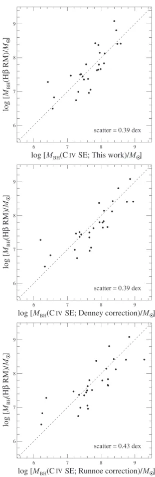
4.2.ComparisonwithP13

Thefinalbest-fitcalibratedequations(Equations(3)and(4)) arevery similartothose ofour previouswork (seeEquations

(2) and (3) of P13). If we compare the two mass estimates basedonboth estimatorsusingthesamemeasurements ofour sample,thereareverysmalloffsets(0.02–0.03dex)withsmall scatters of ∼0.09dex for both FWHM-based and sline-based

masses,whicharemostlycomingfromslightdifferencesinthe slopesbetweenP13andthiswork.Althoughthechangesinthe adoptedvirial relationare modest,it isworthnotingthat this work directlyextendsthe applicabilityoftheCIV-based MBH

estimators toward lower BH masses (~106.5 _M

☉) than were

presentintheP13sample.

4.3.ComparisonwithOtherLinearRegressionMethods

TheadvantagesoftheadoptedstatisticalmodelusingStan inthisworkare(1)usingtheoutlier-robustt-distributionasan alternativetothenormaldistributionforerrordistributionsand

Figure6.PosteriordistributionsoftheresultingparametersofthecalibrationsinFigure 5 forFWHM(left)and sline(right).Theredsolidlinesindicatetheposterior

medianestimate,andthe blackdashedlinesmarkthe uncertaintyranges(i.e., 16%and84%posteriorquantiles).The 2Dmarginaldistributions(black)ofthe

parameterpairsareshownintheoff-diagonalpanels,whilethe1Dmarginalizedhistograms(blue)foreachparameterfromtheposteriorsamplearegiveninthe

diagonalpanels.Thisfigurewasmadeusingthecorner.py(https://github.com/dfm/corner.py).

ourmodel,weprovide acomparison ofresultsby performing the same regression work with other available methods (i.e.,

mlinmix_errandFITEXY).

Figure 9 compares the resulting posterior distributions of parameters obtained from three different regression methods for the same data (i.e., calibration of the FWHM-based estimator using the full sample of 31 local RM AGNs as obtained above).The StanBayesian modelimplemented for this work (Park 2017, in preparation) uses the Student

t-distributions for measurement errors, intrinsic scatter, and thecovariatedistributionmodel.Themlinmix_errmethod, aBayesian linearregressioncodedeveloped byKelly(2007), employsanormalmixturemodelforcovariatedistributionand assumes Gaussian distributions for measurement errors and intrinsic scatter. The FITEXY method, a widely used traditional c2_{-based linear regression method (Tremaine}

etal.2002;seealsoParketal.2012a andreferences therein), also uses Gaussian distributions for measurement errors and intrinsicscatter,butithasnomodelspecifiedforthecovariate distributionand does not take into account possible correla­ tionsbetween measurementerrors.

The left panel in Figure 9 shows an overall consistency ofresults between the Bayesian methods, Stan, and

mlinmix_err,exceptforthedistributionsofintrinsicscatter. Thequitestrongdifferenceofthesintdistributionsisexpected,

because Stan uses t-distributed intrinsic scatter while

mlinmix_errusesnormally distributedintrinsicscatter. By definition,thesintofthet-distributionissmallerthanthatofthe

Gaussian distribution due to the broader tails of the t -distribution (see Kelly et al. 2012 and D. Park 2017, in preparation).Anothernoticeabledifferencebetweentheposter­ ior distributionsis that thewidths of the probability distribu­ tions for theregression parameters obtained from Stan are slightly widerthanthose frommlinmix_err.Although not

significant, this seems toindicatemore reliable uncertainty estimates with Stan, probably due to the flexibility of the adopted t-distributions with degrees-of-freedom parameters. Note that the t-distributionranges widelyfrom the Cauchy distributiontothenormaldistributionwithavarying degrees-of-freedomparameter,butthenumberofGaussiancomponents forthenormalmixturemodelusedinmlinmix_errisfixed asaconstant(e.g.,3bydefault,althoughafewGaussiansare usuallyenough to obtain a reasonable description of theob­ served distributions of many astronomical samples and data, asisthecaseinthis work).

TherightpanelinFigure9alsoshowsaoverallconsistency betweenthe resultingdistributionsofthe BayesianStan and thec2_-basedFITEXY_{method.However,underestimatesofthe}

parameter uncertainties from FITEXY are abit more notice­ able, possibly due to the absence of the covariate model description and not accounting for correlations between measurement errors in FITEXY estimates. The parameter distributionsfromFITEXY areobtainedwith abootstrapping method, soit may not be a consistent comparison with the Bayesian posterior distributions. Manyzero values inthesint

distribution of FITEXY are also noticeable, which indicates that many realizations of bootstrap samples are optimized withouttheadditionofintrinsicscatter.Thisbehaviorisoneof the downsides of the c2_{-based FITEXY estimator, which}

employs asomewhat ad hoc iterative procedure todetermine

sint because it cannot beconstrained simultaneouslywith the

Table4

-1 44 -1

RM M]=a +b log(L1350Å 10 erg s )+g log[DV(CIV ) 1000kms ]

CIVMBHEstimatorCalibrationResultslog[MBH ( )

V IV

D ( ) α β γ sint MeanOffset

(dex)

1σScatter

(dex)

References line s FWHM line s FWHM

6.73±0.01

6.66±0.01

6.71±0.07

7.48±0.24

0.53 0.53

0.50±0.07

0.52±0.09

PreviousCalibrations

2 0.33

2 0.36

2 0.28±0.04

0.56±0.48 0.35±0.05

L L 0.00 0.00 L L 0.295 0.347 VP06 VP06 P13 P13 ThisWork line s FWHM MAD

6.90 _0.340.35 -+

7 54. -+0.270.26

7.15-+0.250.24

0.44 _0.070.07 -+

0 45. -+0.080.08

0.42-+0.070.07

1.66 _0.660.65 -+

0 50. -+0.530.55

1.65-+0.620.61

0.12 _0.060.09 -+

0.16-+0.080.10

0.12-+0.060.09

0.01 0.00 0.00 0.33 0.37 0.33 L

Bestfita

L

ThisWork(Fixingg =2)

line s

FWHM MAD

6.73-+0.070.07

6.84-+0.090.09

7 01. -+0.070.07

0 43. -+0.060.06

0.33-+0.070.07

0 41. -+0.060.06

2

2

2

0.12-+0.060.09

0.22-+0.100.11

0.12-+0.060.09

0.01 −0.01 0.00 0.33 0.43 0.33

Bestfita

L

Bestfita

ThisWork(Fixingb =0.5)

line s

FWHM MAD

6.99-+0.340.34

7.62 _0.230.23 -+

7.23-+0.240.24

0.5 0.5 0.5

1.49-+0.620.63

0.31_0.450.46 -+

1.41-+0.580.57

0.12-+0.060.09

0.16 _0.080.10 -+

0.12-+0.060.09

0.01 0.01 0.01 0.34 0.38 0.34 L L L

ThisWork(Fixingb =0.5andg =2)

line s

FWHM MAD

6.72 _0.070.07 -+

6.82-+0.090.09

7.00-+0.070.07

0.5 0.5 0.5 2 2 2

0.12 _0.060.08 -+

0.26-+0.110.11

0.12-+0.060.09

0.01 0.00 0.01 0.35 0.47 0.35 L L L

Note.Themeanoffsetand1s scatterforourcalibrationsaremeasuredfromtheaverageandstandarddeviationsofmassresidualsbetweentheRMmassesand

calibratedSEmasses,D =logMBH(RM)-logMBH(SE).Notethattheapparentbigdifferencein sintestimatesbetweenthepreviouscalibrationsandthisworkis

mostlyduetothedifferencesintheadoptedRMmasserrorandstatisticalmodel.Theuncertaintyoflogf (i.e.,0.31dex)isaddedinquadraturetotheuncertaintiesof

theRMBHmassesinthiswork.Thestandarddeviation(σ)ofthe t-distributionisbydefinitiondifferent(larger)fromthatoftheGaussiandistributionduetothe

heavytailwhenthedegrees-of-freedomparameterissmall.Inthiscase,the sint

t-distribution.Boldfacefontindicatesbit-fitvalues.

a

WesuggestthesecalibrationsasthebestMBHestimators.

and luminosities)arevery smallinthiswork (i.e.,onlyafew percent, on average, due to high-quality HST spectra). The resulting covariances between measurement errors are conse­ quentlyverysmallaswell,thusleadingtovirtuallynoeffectof error correlations onthe regressionparameter estimates, even thoughtherearecorrelationsbetweenmeasurementerrors(see Table 3). To summarize, all three methods (Stan, mlin­

mix_err, andFITEXY) produce consistent results in this work, exceptforarguablymore reliableparameteruncertainty estimateswhenusingStan,giventhesmallmeasure­

ment errors of the covariates. Although the differenceismarginal inthiswork, moreflexiblet-distributed errors, as well as anexplicit covariate model description, are generally recommended to get a correct central trend against outliers by avoiding theeffects of possible unaccounted systematic errors(seePark 2017,inpreparation,fordetails).

4.4. MAD-BasedCalibration

Although we prefer line dispersion (sline) to FWHM in

measuringCIV linewidth,asinvestigatedabove,onedownside

parameterofthe t-distributionmodelisnotthesameasthedataspread(σ)ofthe

ofusingslineisthatitrequires high-S/Ndatatoaccuratelyfit

the line wings. Noisy data can lead to biases in line width measurements, especially when the line profile has very extended wings, as istypical of CIV lines (Denney et al. 2013;seealsoFine etal. 2010).

Figure 7. Three-dimensional representation of the calibration results of Figure 5 for clarification.Red circlesindicateobserved data.Colored tilted planes

representtheresultingcalibrationwithEquation(2).Blackverticallinesconnectingthedatapointstothefittedplaneshowthemassdeviationbetweentheobserved

RMmassandcalibratedSEmass.

Figure8.ComparisonoftheSECIVvelocitywidthmeasurements,FWHM(left)and sline(right),totheobservedRMmasses.

important when using low-S/N data, which makes accurate characterizationof linewingsvery difficult.

Thus,theMADinheritssomeofthepracticalmeritsofboth

slineandFWHMandpossiblyworksbetterinlow-qualitydata.

WehavecarriedoutMADmeasurementsforthebroadlinesin our sample,and we findgood consistencybetween theMAD andslinemeasurements(Figure10).Thetwomeasurementsare

very nicely correlated with a marginal scatter, while a poor

correlationwithalargescatterisobservedbetweentheFWHM andMAD.Inthisregard,theMADmaybethebestlinewidth measurement method for theCIV emission line when using survey-qualityspectra,asadvocatedbyDenneyetal.(2016b). As it is for the case of sline, the γ of theMAD is also

Figure9.ComparisonsoftheresultingposteriordistributionsusingStantothoseusingmlinmix_err(left)andFITEXY(right).Theone- andtwo-dimensional

⎞ ⎠

distributionsofaparameter(diagonalpanels)andparameterpairs(off-diagonalpanels)areshownwiththekerneldensityestimateusingtheGetDist(https://

github.com/cmbant/getdist)pythonpackage.Notethatsomeamountofsmoothinghasbeenappliedforclarityofcomparisonbetweenthedistributions.

estimatorbasedontheMADasthemeasureofCIV linewidth: andthedifficultyofobtainingspace-basedUVmonitoringdata

⎛ ⎝

⎢ ⎥⎤_⎦ ⎜ ⎟

⎡ ⎣

forlow-zAGNs.

Instead, Coatman etal. (2016, 2017; see also Shen& Liu

SE

( ) l

MBH +0.07 +0.06 L1350Å

7.01 0.41

= +

log -0.07 -0.06 log 2012) recentlyprovided a new empirical correction to

1044_{erg s} 1

M - _{CIV FWHM-basedBH massestimators as afunction of CIV}

⎤ ⎦

⎢ ⎥

5 ( )

⎡ ⎣

Inthiscase,theoverallscatteragainstRMmassesis0.33dex. The resulting MAD-based calibration and posterior distribu­ tions, which are not shown here, are very similar to the

sline-based,exceptforaslightdifferenceintheinterceptα(see

Table4).

4.5.PossibleBiasesDuetoCIVBlueshift

In our calibration sample (i.e., local RM AGNs), CIV blueshifts arebasicallyinsignificant(seeRichardsetal.2011; Shen2013), soourcalibrationbasedonthelocalRMAGNsis relativelyfreeofpossiblebiasesstemmingfromtheeffectofa largeblueshift.However,theapplicabilityofthiscalibrationto high-zquasarsmaybeuncertain,becauselargeCIV blueshifts are known to be common in high-z, high-luminosity quasars

(see, e.g., Richards et al. 2002). Available CIV-based MBH

estimators have been usedfor measuringtheBHmasses ofa statistical sample of such high-z AGNs, simply based on assumption and extrapolation without a direct test. The best way of investigating and possibly correcting for the effect of CIV blueshifts on BHmass estimates would be tousedirect CIV RMdata(seeDenney2012forthecaseof localAGNs). The number of AGNs withdirect CIV RM observations is,

MAD (C IV)

+2 log _-1 .

1000 km s

blueshift by comparing SE CIV measurements to SE Hα measurements.

In Figure 11, we compare the overall distributions of CIV FWHM-basedBHmassestimatesasafunctionofCIV blueshift usingthespectral measurements ofDR9 BOSSquasars.15 The blue shaded contour presents BH masses computed from the blueshift-corrected formula from Coatman et al. (2017), whiletheredand greenshadedcontoursshowthosecalculated with theupdated recipe in this work and the original VP06 equation, respectively. As can be seen, at alarge blueshift

(2000kms−1),ourestimator,whichdoesnottakeintoaccount theCIV blueshift, produces a similar mass distribution to the blueshift-correcteddistribution. Notethat theoverestimated BH massesfromtheVP06estimatorarereducedbycorrectingforthe blueshifteffectontheCIV FWHM(Coatmanetal.2017). Thus, ourlocallycalibratedFWHM-basedMBHestimatorisapplicable

to a sample of high-z, high-luminosity quasars withhigh CIV blueshifts(e.g.,2000kms−1),givingaconsistentmassscaleon average.

At asmall blueshfit range(~0 – 1000 kms−1), where our calibration sample is distributed, the overall massscale from ourestimatorissmallerthanthoseofVP06andCoatmanetal.

108.5

(2017)in the high-mass regime ( M M☉) and larger in

108.5

the low-mass regime ( M M☉). This trend has been described in detail by P13. Arguably, our calibration in this work(andP13)hasresultedinabetteragreement(overallmass scale)withRMmassesthanthatofVP06intermsofintrinsic