Establishment of Preliminary Test Estimators and Preliminary Test Confidence Intervals for Measures of Reliability of an Exponentiated Distribution Based on Type-II Censoring

ESTABLISHMENT OF PRELIMINARY TEST ESTIMATORS AND

PRELIMINARY TEST CONFIDENCE INTERVALS FOR

MEASURES OF RELIABILITY OF AN EXPONENTIATED

DISTRIBUTION BASED ON TYPE-II CENSORING

Ajit Chaturvedi

Department of Statistics, University of Delhi, Delhi 110007, India

Anshika Bhatnagar1

Department of Statistics, University of Delhi, Delhi 110007, India

1. INTRODUCTION

Life testing experiments are usually time consuming and expensive in nature. To reduce the cost and time of experimentation, various types of censoring schemes are used in the life testing experiments. This paper dwells on Type-II censoring scheme for developing preliminary test estimators (PTEs) and preliminary test confidence intervals (PTCIs) for the parameters and measures of reliability with respect to exponentiated distributions.

The reliability functionR(t)is defined as the probability of failure-free operation until timet. Thus, if the random variableX denotes the lifetime of an item or a sys-tem, thenR(t) =P(X >t). Another measure of reliability under stress strength setup is the probabilityP =P(X >Y), which represents the reliability of an item or a sys-tem of random strengthX subject to random stressY. For details of work existing in literature, one may refer to Bartholomew (1957, 1963), Pugh (1963), Basu (1964), Tong (1974, 1975), Johnson (1975), Kellyet al.(1976), Sathe and Shah (1981), Chao (1982), Awad and Gharraf (1986), Tyagi and Bhattacharya (1989), Chaturvedi and Rani (1997, 1998), Chaturvedi and Surinder (1999), Chaturvedi and Tomer (2002, 2003), Chaturvedi and Singh (2006, 2008), Chaturvedi and Pathak (2012, 2013, 2014) and Chaturvedi and Malhotra (2016, 2017, 2018).

Quite often we come across cases in which there exists some prior information in re-spect of parameters, which may ultimately lead to improved inferential results. It is well known that the estimators with the prior information (called the restricted estimators) perform better than the estimators with no prior information (called the unrestricted estimators).

However, when the prior information is doubtful (or not sure), one may combine the restricted and unrestricted estimator to obtain an estimator with better performance, which leads to the PTEs. The preliminary test approach was first discussed by Bancroft (1944) and further advancements were proposed by Sen and Saleh (1978), Saleh and Kib-ria (1993), KibKib-ria (2004), KibKib-ria and Saleh (1993, 2004, 2005, 2006, 2010), Saleh (2006) and Belaghiet al.(2014, 2015).

A lot of research work related with reliability estimation of different distributions has taken place. For a brief review, one may refer to Ljubo (1965), Tadikamalla (1980), Mudholkar and Srivastava (1993), Mudholkaret al.(1995), Mudholkar and Hutson (1996), Guptaet al.(1998), Gupta and Kundu (1999, 2001a,b, 2002, 2003a,b), Jiang and Murthy (1999), Guptaet al.(2002), Xieet al.(2002), Raqab (2002), Nassar and Eissa (2003, 2004), Laiet al.(2003), Kunduet al.(2005), Kundu and Gupta (2005), Kundu and Raqab (2005), Palet al.(2006, 2007), Abdel-Hamid and AL-Hussaini (2009), Shawky and Abu-Zinadah (2009), AL-Hussaini (2010), AL-Hussaini and Hussein (2011), Abdul-Moniem and Abdel-Hameed (2012) and Chaturvedi and Vyas (2017).

In the present paper, we have dealt with an overview of exponentiated distributions in Section 2. The relevant results on the uniformly minimum variance unbiased estima-tors (UMVUEs) and the maximum likelihood estimaestima-tors (MLEs) of parameterσraised to certain power p, the measures of reliability functions, namely, R(t) and P under Type-II censoring, as available in literature are reproduced in Section 3 for quick refer-ence and use by us subsequently. In Section 4, we develop the PTEs for parameterσ raised to certain power p,R(t)andP respectively based on their UMVUEs and MLEs. In Section 5, we derive the PTCIs for the parameterσ,R(t)andPbesides obtaining the expression of coverage probability of the PTCI for the parameter ‘σ’. Finally, Section 6 depicts the supporting numerical results.

2. EXPONENTIATED DISTRIBUTIONS

Let us consider a positive random variable X, with cumulative distribution function (cdf)F(x). Then, forσ >0,

G(x) = [F(x)]σ (1)

is also a cdf. Such distributions are referred to as exponentiated distributions. Denoting by f(x), the probability density function corresponding toF(x), we can write

g(x) =σ[F(x)]σ−1f(x). (2) Let us suppose thatn items are put on life testing and failure of only firstr items are observed. Let us denote the r observed failure times byX₍₁₎ ≤X₍₂₎≤. . .≤X_(r),(0<

r≤n)which implies that(n−r)items have survived untilX_(r).

Using (2), the joint pdf ofnorder statisticsX₍₁₎≤X₍₂₎≤. . .≤X_(n)is given by

g∗(x₍₁₎,x₍₂₎, . . . ,x_(n);σ) =n!σn n

Y

i=1

or

g∗(x₍₁₎,x₍₂₎, . . . ,x_(n);σ) =n!σn n

Y

i=1

exp{−σ(−logF(x_(i)))}

‚_f(_x (i))

F(x_(i))

Œ

. (4)

Considering the transformation,y_(i)=−logF(x_(i)), the joint pdf ofY₍₁₎≤Y₍₂₎≤. . .≤

Y_(n), is given by

h∗(y₍₁₎,y₍₂₎, . . . ,y_(n);σ) =n!σnexp

‚

−σ

n

X

i=1 y_(i)

Œ

(5)

on integrating outY_(r+1)≤Y_(r+2)≤. . .≤Y_(n) from (5), the joint pdf ofY₍₁₎≤Y₍₂₎ ≤

. . .≤Y_(r)is as follows

h∗∗(y₍₁₎,y₍₂₎, . . . ,y_(r);σ) =n(n−1). . .(n−r+1)σnexp

¨

−σ

‚ _r

X

i=1

y_(i)+ (n−r)y_(r)

Œ«

.

SinceF(x_i), being cdf, follows theU(0, 1)distribution,−logF(x_(i))follows the expo-nential distribution with mean life 1/σ.

Consider the transformationZ_i= (n−i+1)(Y_(i)−Y_(i−1)),i=1, 2, . . . ,r

⇒

r

X

i=1 z_i=

‚ _r

X

i=1

y_(i)+ (n−r)y_(r)

Œ

=S_r.

S_r, being the sum of exponential variates, follows the gamma distribution with pdf

t(s_r,σ) = σ r

Γ_r srr−1exp(−σsr). (6)

3. AVAILABLE RESULTS ON CLASSICAL ESTIMATION

In the present paper, we intend to utilize appropriately certain results on UMVUE and MLE forσp_{,R(t)andP, derived by Chaturvedi and Vyas (2017). These are consolidated} and reproduced below for quick reference through Result 1 and Result 2.

RESULT1. The UMVUE and MLE ofσpand R(t)are as follows: (i) For(p6=0), the UMVUE ofσp_{, i.e.}

b

σp U=

Γr

Γ₍r−p)

(ii) For(p6=0), the MLE ofσp_{, i.e.}

b

σp M L=

r S_r

p

.

(iii) The UMVUE of R(t), i.e.

b

R_U(t) =1−

1+logF(t) S_r

r−1

; −logF(t)<S_r.

(iv) The MLE of R(t), i.e.

b

R_{M L}(t) =1−(F(t))Srr _.

SupposeX and Y are two independent random variables following the classes of distributiong₁(x;σ₁)andg₂(y;σ₂), respectively, where

g₁(x;σ₁) =σ₁F₁(x)σ1−1f₁(x), g₂(y;σ2) =σ2F2(y)σ2−1f2(y).

Let us suppose thatnand mitems are put on test corresponding toX andY, respec-tively. Further, the failure times of r andl units are observed fromX andY, respec-tively.

As done earlier,S_r=Pr

j=1

Y_1(j)+ (n−r)Y_1(r)andT_l=Pl

j=1

Y_2(j)+ (m−l)Y_2(l).

RESULT2. The UMVUE and MLE of P are respectively as follows:

(i) The UMVUE, i.e.

b

P_U=



    

    

(l−1)

Z Sr

Tl

0

(1−z)l−2

–

1−

1−Tl

S_rz

r−1™

, S_r <T_l,

(l−1)

Z1

0

(1−z)l−2

–

1−

1−Tl

S_rz

r−1™

, S_r ¾Tl.

(ii) The MLE, i.e.

b

4. PROPOSED PRELIMINARY TEST ESTIMATORS

Let us suppose that the prior information of the parameter can be expressed in the form of following hypothesis

H₀:σ=σ₀ against H₁:σ6=σ0.

From (6), we know that

2σS_r∼χ22r. (7)

Therefore, the critical region is given by

(0<S_r <k₀)∪(k₁<S_r<∞),

where k₀ = ₂1_σ 0χ

2 2r

α 2

,k₁ = ₂1_σ 0χ

2 2r 1−

α 2

and αis the level of significance. Let us suppose

χ2 2r

α

2

=C₂ and χ₂2_r1−α

2

=C₁ (8)

andI(A)be the indicator function of the following set

A={χ22r;C2≤χ22r≤C1}.

The PTEs ofσpbased on UMVUE and MLE are then given respectively by

b

σp P T_U=σb

p U−(σb

p U−σ

p

0)I(A) (9)

and

b

σp

P T_M L=σb

p M L−(σb

p M L−σ

p

0)I(A), (10)

whereσb

p Uandσb

p

M Lare as defined in Result 1(i) and Result 1(ii), respectively.

Next, we find the PTEs ofR(t)andP based on UMVUEs and MLEs. Using Re-sult 1(iii) and ReRe-sult 1(iv) on the UMVUE and MLE ofR(t), the PTEs ofR(t)based on UMVUE and MLE are given respectively by

b

R_{P T_U}(t) =Rb_U(t)−(Rb_U(t)−R₀(t))I(A), (11)

whereR₀(t) =1−F(t)σ0, underH

0and

b

R_{P T_M L}(t) =Rb_{M L}(t)−(Rb_{M L}(t)−R₀(t))I(A). (12)

Let us now derive the PTEs ofP based on UMVUE and MLE. We know that

P= σ1 σ1+σ2

Suppose, we want to test

H₀:P=P₀ against H₁:P6=P₀

P=P₀ gives σ₁=kσ₂ where k= P0 1−P₀.

Therefore,H₀is equivalent to

H₀:σ₁=kσ₂ against H₁:σ₁6=kσ₂. We know that

2σ₁S_r∼χ22r and 2σ2Tl∼χ22l. Therefore,

σ1Srl

σ2Tlr

∼F_2r,2l. (13)

The critical region for testingH₀:P=P₀is given by

S_r T_l <k2

∪

k₃<Sr T_l

,

where

k₂= r k lF2r,2l

α

2

and k₃= r k lF2r,2l

1−α

2

. (14)

LetI(B)be indicator function of the set

B={F_2r,2l;C₄≤F_2r,2l≤C₃},

whereC₃=F_2r,2l 1−α₂

;C₄=F_2r,2l α₂

.

As seen earlier in Result 2(i) and Result 2(ii), the UMVUE and MLE ofPwhenX, Y belong to same family of distribution are respectively given by

b

P_U=



    

    

(l−1)

Z Sr_Tl

0

(1−z)l−2

1−

§

1−Tl

S r z

ªr−1

, S_r<T_l,

(l−1)

Z1

0

(1−z)l−2

–

1−

1−Tl

S_rz

r−1™

, S_r¾T_l

and

b

The PTEs ofPbased on UMVUE and MLE are then obtained respectively by

b

P_{P T_U}=Pb_U−(Pb_U−P₀)I(B) (15)

and

b

P_{P T_M L}=Pb_{M L}−(Pb_{M L}−P₀)I(B), (16)

whereP₀is the assumed value ofPunderH₀.

5. PRELIMINARY TEST CONFIDENCE INTERVALS

In this section, we derive the PTCIs for σ,R(t)andP based on their UMVUEs and MLEs.

From (7), we know that, 2σS_r∼χ2 2r

⇒ P

¨

χ2 2r

α 2

2S_r < σ <

χ2 2r 1−

α 2

2S_r

«

=1−α, (17)

whereαis the significance level.

From Result 1(i) and Result 1(ii), we know thatσbU= r−1

Sr andσbM L= r

Sr, therefore, 100(1−α)% equal tail confidence interval (CI) forσbased on UMVUE and MLE may be written as

I_{ET_σ_U}=

–_χ2

2r

α 2

2(r−1)σbU,

χ2 2r 1−

α 2

2(r−1) σbU ™

(18)

and

I_{ET_σ_M L}=

–_χ2

2r α2

2r σbM L,

χ2 2r 1−α2

2r σbM L ™

. (19)

The proposed PTCI ofσbased on UMVUE and MLE are as follows:

I_{P T_σ_U}=

–_χ2

2r α2

2(r−1)σbP T_U,

χ2 2r 1−α2

2(r−1) σbP T_U ™

(20)

I_{P T_σ_M L}=

–_χ2 2r

α 2

2r σbP T_M L,

χ2 2r 1−

α 2

2r σbP T_M L ™

, (21)

whereσbP T_UandσbP T_M Lare as defined in (9) and (10), respectively. Next we derive the PTCI forR(t). Using (1), we know that

Using (17) and (22), we can write

P

¨

1−exp

‚

χ2 2r

α 2

2S_r logF(t)

Œ

<R(t)<1−exp

‚

χ2 2r 1−

α 2

2S_r logF(t)

Œ«

=1−α.

Therefore, 100(1−α)% equal tail CI forR(t)may be written as

I_{ET_R}=

–

1−exp

‚

χ2 2r

α 2

2S_r logF(t)

Œ

, 1−exp

‚

χ2 2r 1−

α 2

2S_r logF(t)

Ϊ

. (23)

From Result 1(iii), we can write

logF(t)

S_r = (1−RbU(t)) 1

r−1−1. (24)

Using (24) in (23), 100(1−α)% equal tail CI for R(t)based on UMVUE may be written as

I_{ET_R_U}=

–

1−exp

¨_χ2

2r

α 2

2 ((1−RbU(t)) 1 r−1−1)

«

,

1−exp

¨_χ2

2r 1−

α 2

2 ((1−RbU(t)) 1 r−1−1)

«™

From Result 1(iv), we can write

logF(t) =Sr

r log(1−RbM L(t)). (25)

Using (25) in (23), 100(1−α)% equal tail CI forR(t)based on MLE may be written as

I_{ET_R_M L}=

–

1−exp

¨_χ2

2r α2

2r log(1−RbM L(t))

«

,

1−exp

¨_χ2 2r 1−

α 2

2r log(1−RbM L(t))

«™

The proposed PTCIs ofR(t)based on its UMVUE and MLE are as follows:

I_{P T_R_U}=

–

1−exp

¨_χ2

2r α2

2 (1−RbP T_U(t)) 1 r−1−1

«

,

1−exp

¨_χ2

2r 1−

α 2

2 ((1−RbP T_U(t)) 1 r−1−1)

«™

I_{P T_R_M L}=

–

1−exp

¨_χ2

2r

α 2

2r log(1−RbP T_M L(t))

«

,

1−exp

¨_χ2

2r 1−α2

2r log(1−RbP T_M L(t))

«™

.

Now, we derive the CI forP. We know thatP= σ1

σ1+σ2

= 1

1+σ2

σ1

and from (13),

σ₂T_lr

σ1Srl

∼F_2l,2r using the same approach as above, 100(1−α)% equal tail CI forPmay be written as

I_{ET_P}=





1

1+ l Sr

r TlF2l,2r 1−

α 2

,

1

1+ l Sr r TlF2l,2r

α 2



. (26)

From Result 2(i), we can write

S_r T_l =

         b P_U

d1−d2+d3−d4, Sr<Tl,

b

P_U

1−d5, Tl¶Sr,

(27)

where

d1=Tl S_r ,

d2= l−1

X

i=0

(−1)i (l−1)!

i!(l−i−1)!

_S

r T_l

i−1

,

d3= l−2

X

i=0

(−1)i (l−1)!

(i+1)!(l−i−2)!

_S

r T_l

i

,

d4= l−2

X

i=0

(−1)i₍ (l−1)!(r−1)!

i+r)!(l−i−2)!

_S

r T_l

i

,

d5= r−1

X

i=0

(−1)i (l−1)!(r−1)! (r−1−i)!(l+i−1)!

T_l S_r

i+1

Using (27) in (26), we can write 100(1−α)% equal tail CI forPbased on UMVUE as

I_{ET_P_U}

=                    1

1+ l_r Pb_U

(d1−d2+d3−d4)F2l,2r 1−α2

, 1

1+l_r Pb_U

(d1−d2+d3−d4)F2l,2r α2



, S_r<T_l 



1

1+_rl Pb_U

(1−d5)F2l,2r 1−α2

, 1

1+_rl Pb_U

(1−d5)F2l,2r α2



, S_r¾T_l

From Result 2(ii), we can write

l S_r r T_l =

1−Pb_{M L}

b

P_{M L} . (28)

Using (28) in (26), we can write 100(1−α)% equal tail CI forPbased on MLE as

I_{ET_P_M L}=



 

1

1+n1−Pb_{M L} b

PM L

o

F_2l,2r 1−α₂

, 1

1+n1−Pb_{M L} b

PM L

F_2l,2r α₂o 

 .

The proposed PTCIs ofP based on its UMVUE and MLE are then as follows:

I_{P T_P_U}

=                       1

1+ l_r Pb_{P T_U}

(d1−d2+d3−d4)F2l,2r 1−α2

, 1

1+l_r Pb_{P T_U}

(d1−d2+d3−d4)F2l,2r α2





, Sr<Tl 

 

1

1+_rl Pb_{P T_U}

(1−d5)F2l,2r 1−α2

, 1

1+_rl Pb_{P T_U}

(1−d5)F2l,2r α2





, Sr¾Tl

I_{P T_P_M L}=



  

1

1+§1−Pb_{P T_M L} b

PP T_M L

ª

F_2l,2r 1−α₂

, 1

1+§1−Pb_{P T_M L} b

PP T_M L

ª

F_2l,2r α₂ 

  

We know thatT =2σS_r∼χ2 2r

P(σ∈I_{P T_σ_U}) =P

n

σ∈(a₁σ₀,a₂σ₀),χ₂2_r

α

2

<2σ₀S_r < χ₂2_r

1−α

2

o

+Pnσ∈(a₁σ_bU,a2σbU), 2σ0Sr< χ

2 2r

α

2

o

+Pnσ∈(a₁σ_bU,a2σbU), 2σ0Sr> χ

2 2r

1−α

2

o

,

wherea₁= χ2r2(α2)

2(r−1) anda2= χ2r(2 ₁₋α

2)

2(r−1) .

Denotingδ=_σσ

0, we get

P(σ∈I_{P T_σ_U}) =Pna₁< δ <a₂;δχ₂2_rα 2

<T< δχ₂2_r1−α

2

o

+Pnχ₂2_rα 2

<T< χ₂2_r1−α

2

;T < δχ₂2_rα 2

o

+Pnχ₂2_rα 2

<T< χ₂2_r1−α

2

;T > δχ₂2_m1−α

2

o

or

P(σ∈I_{P T_σ_U}) =P

n δχ2 2r α 2

<T < δχ₂2_r

1−α

2

I_a 1a2(δ) +P n χ2 2r α 2

<T <min

χ2 2r

1−α

2

,δχ₂2_r

α

2

o

+Pnmax

χ2 2r α 2

,δχ₂2_r

1−α

2

<T < χ2 2r

1−α

2

o

.

Let us denoteP

δχ2 2r α2

<T < δχ2

2r 1−α2 Ia1a2(δ)byA. Considering all possible cases ofδ, we may write

P(σ∈I_{P T_σ_U}) =

                    

A+1−α, 0< δ≤ χ2r2(

α

2)

χ2 2r(1−

α

2)

A+1−α, δ >χ

2 2r(1−α2)

χ2 2r(

α

2)

A+P

χ2 2r α2

<T < δχ2

2r α2 , 1< δ≤ χ2

2r(1−α2)

χ2 2r(

α

2)

A+P

δχ2 2r 1−α2

<T < χ2

2r 1−α2 , χ2

2r(α2)

χ2 2r(1−α2)

< δ≤1

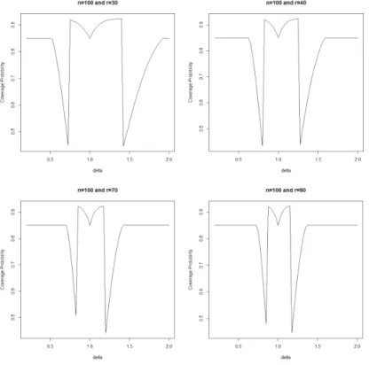
Similarly, coverage probability for other PTCI may be obtained.

6. NUMERICAL FINDINGS

noted here thatG(x), being the cdf, follows the uniform distribution. Further suppose thatX_i’s, the failure times of experimental units, follow the Weibull distribution with shape parameterγ=1.25 and scale parameterλ=10.

Estimates ofσ

For each combination of r and p, the UMVUEs and MLEs ofσare obtained. PTEs ofσ based on UMVUEs and MLEs are further obtained. We replicated this process 1500 times in order to obtain 1500 estimates. Thereafter mean value of estimates and corresponding mean square error (MSE) are obtained using these 1500 estimates. The results are shown in Table 1. From Table 1 it may be observed that PTEs are more close to the actual value of parameter and their MSE is less than the MSE of traditional UMVUEs and MLEs, thereby establishing superiority of PTEs. Also, it is observed that as r increases, PTEs tend to get closer to the true value.

Estimates of R(t)

For each combination of r and t, the UMVUEs, MLEs and PTEs ofR(t)based on UMVUE, MLE are obtained using the similar approach as mentioned above. The MSE for each estimator is further obtained. The results may be seen in Table 2 and it may be observed that PTEs are more close to the actual value ofR(t)and their MSE is less than the MSE of traditional UMVUEs and MLEs ofR(t).

Estimates of P

For each combination of(r,l)and p, the UMVUEs, MLEs and PTEs ofP based on UMVUE, MLE are obtained besides the MSE for each estimator using the similar ap-proach as mentioned above. The results may be seen in Table 3. Similar observations as above may be drawn from Table 3 as well. Therefore, we may conclude that the PTEs perform better than the classical estimators as the MSE of the PTEs is observed to be less than the MSE of the classical estimators under the simulated data set.

TABLE 1

Estimates and corresponding mean square error of the parameterσ. The values are truncated to 4 decimal points, therefore few values in the column of mean square error being very small are

mentioned as 0.0000.

r p Estimates Mean square error

b

σU bσP T_U σbM L σbP T_M L M SE(σbU) M SE(σbP T_U) M SE(σbM L) M SE(σbP T_M L)

2 0.5052 1.4549 0.5340 1.4562 0.0696 0.0020 0.0778 0.0019 55 4 0.2414 1.4361 0.2911 1.4384 0.0140 0.0041 0.0203 0.0038 5 0.1670 1.4427 0.2214 1.4448 0.0096 0.0033 0.0169 0.0030 2 0.6380 1.4641 0.6712 1.4654 0.0107 0.0013 0.0118 0.0011 60 4 0.3926 1.4433 0.4658 1.4471 0.0582 0.0032 0.0819 0.0028 5 0.3118 1.4524 0.4036 1.4558 0.0196 0.0023 0.0328 0.0020 2 1.1625 1.4862 1.2105 1.4883 0.0770 0.0002 0.0835 0.0001 75 4 1.3126 1.4873 1.5039 1.4973 0.0530 0.0002 0.0696 7.5217 5 1.4376 1.4947 1.7648 1.5124 0.3609 0.0000 0.5439 0.0002

TABLE 2

Estimates and corresponding mean square error of R(t). The values are truncated to 4 decimal points, therefore few values in the column of mean square error being very small are mentioned as

0.0000.

r t R(t) Estimates Mean Square Error

b

RU(t) Rb_{P T_U}(t) Rb_{M L}(t) Rb_{P T_M L}(t) M SE(Rb_U(t)) M SE(Rb_{P T_U}(t)) M SE(Rb_{M L}(t)) M SE(Rb_{P T_M L}(t)) 1.5 0.9092 0.8210 0.9044 0.8218 0.9045 0.0008 0.0000 0.0007 0.0000 55 2 0.8729 0.7722 0.8686 0.7737 0.8687 0.0009 0.0000 0.0009 0.0000 3 0.7987 0.6814 0.7924 0.6842 0.7925 0.0069 0.0000 0.0067 0.0000 1.5 0.9092 0.8555 0.9068 0.8557 0.9068 0.0003 0.0000 0.0003 0.0000 60 2 0.8729 0.8108 0.8694 0.8116 0.8694 0.0013 0.0000 0.0013 0.0000 3 0.7987 0.7256 0.7954 0.7277 0.7955 0.0001 0.0000 0.0001 0.0000 1.5 0.9092 0.9259 0.9102 0.9251 0.9101 0.0001 0.0000 0.0001 0.0000 75 2 0.8729 0.8933 0.8740 0.8929 0.8740 0.0000 0.0000 0.0000 0.0000 3 0.7987 0.8239 0.8005 0.8244 0.8005 0.0033 0.0000 0.0032 0.0000

TABLE 3

Estimates and corresponding mean square error of P . The values are truncated to 4 decimal points, therefore few values in the column of mean square error being very small are mentioned as 0.0000.

(r,l) p P Estimates Mean Square Error

b

Figure 1 –Coverage probability of PTCI ofσplotted as a function of delta.

ACKNOWLEDGEMENTS

The authors gratefully acknowledge the suggestions given by the anonymous referee(s), which have immensely helped to improve the presentation of the paper.

REFERENCES

A. H. ABDEL-HAMID, E. K. AL-HUSSAINI(2009). Estimation in step-stress accelerated life tests for the exponentiated exponential distribution with Type I censoring. Compu-tational Statistics and Data Analysis, 53, pp. 1328–1338.

I. B. ABDUL-MONIEM, H. F. ABDEL-HAMEED(2012).On exponentiated Lomax distri-bution. International Journal of Mathematical Archive, 3, no. 5, pp. 2144–2150.

E. K. AL-HUSSAINI(2010).On exponentiated class of distributions. Journal of Statistical

E. K. AL-HUSSAINI, M. HUSSEIN(2011).Bayes prediction of future observables from ex-ponentiated populations with fixed and random sample size. Open Journal of Statistics, 1, pp. 24–32.

A. M. AWAD, M. K. GHARRAF(1986). Estimation of P(Y <X)in the Burr case: A comparative study. Communications in Statistics - Simulation and Computation, 15, no. 2, pp. 389–403.

T. A. BANCROFT(1944). On biases in estimation due to the use of preliminary tests of significance. The Annals of Mathematical Statistics, 15, no. 2, pp. 190–204.

D. J. BARTHOLOMEW(1957). A problem in life testing. Journal of the American Statis-tical Association, 52, pp. 350–355.

D. J. BARTHOLOMEW (1963). The sampling distribution of an estimate arising in life testing. Technometrics, 5, pp. 361–374.

A. P. BASU (1964). Estimates of reliability for some distributions useful in life testing.

Technometrics, 6, pp. 215–219.

R. A. BELAGHI, M. ARASHI, S. M. M. TABATABAEY(2014). Improved confidence in-tervals for the scale parameter of Burr XII model based on record values. Computational Statistics, 29, no. 5, pp. 1153–1173.

R. A. BELAGHI, M. ARASHI, S. M. M. TABATABAEY(2015).On the construction of pre-liminary test estimator based on record values for the Burr XII model. Communications in Statistics - Theory and Methods, 44, no. 1, pp. 1–23.

A. CHAO(1982). On comparing estimators of p r{X>Y}in the exponential case. IEEE Transactions on Reliability, R-26, pp. 389–392.

A. CHATURVEDI, A. MALHOTRA(2016). Estimation and testing procedures for the re-liability functions of a family of lifetime distributions based on records. International Journal of System Assurance Engineering and Management, 8, no. 2, pp. 836–848.

A. CHATURVEDI, A. MALHOTRA(2017). Inference on the parameters and reliability characteristics of three parameter Burr distribution based on records. Applied Mathe-matics and Information Sciences, 11, no. 3, pp. 837–849.

A. CHATURVEDI, A. MALHOTRA(2018). On the construction of preliminary test esti-mators of the reliability characteristics for the exponential distribution based on records. American Journal of Mathematical and Management Sciences, 37, no. 2, pp. 168–187.

A. CHATURVEDI, A. PATHAK(2013).Bayesian estimation procedures for three parameter exponentiated Weibull distribution under entropy loss function and Type II censoring.

URLinterstat.statjournals.net/YEAR/2013/abstracts/1306001.php.

A. CHATURVEDI, A. PATHAK (2014). Estimation of the reliability function for four-parameter exponentiated generalized Lomax distribution. International Journal of Sci-entific & Engineering Research, 5, no. 1, pp. 1171–1180.

A. CHATURVEDI, U. RANI(1997).Estimation procedures for a family of density functions representing various life-testing models. Metrika, 46, pp. 213–219.

A. CHATURVEDI, U. RANI(1998). Classical and Bayesian reliability estimation of the generalized Maxwell failure distribution. Journal of Statistical Research, 32, pp. 113– 120.

A. CHATURVEDI, K. G. SINGH(2006). Bayesian estimation procedures for a family of lifetime distributions under squared-error and entropy losses. Metron, 64, no. 2, pp. 179–198.

A. CHATURVEDI, K. G. SINGH(2008).A family of lifetime distributions and related esti-mation and testing procedures for the reliability function. Journal of Applied Statistical Science, 16, no. 2, pp. 35–50.

A. CHATURVEDI, K. SURINDER(1999). Further remarks on estimating the reliability function of exponential distribution under Type-I and Type II censorings. Brazilian Jour-nal of Probability and Statistics, 13, pp. 29–39.

A. CHATURVEDI, S. K. TOMER(2002). Classical and Bayesian reliability estimation of the negative binomial distribution. Journal of Applied Statistical Science, 11, pp. 33– 43.

A. CHATURVEDI, S. K. TOMER(2003). UMVU estimation of the reliability function of the generalized life distributions. Statistical Papers, 44, no. 3, pp. 301–313.

A. CHATURVEDI, S. VYAS(2017). Estimation and testing procedures for the reliability functions of exponentiated distributions under censorings. Statistica, 77, no. 3, pp. 207– 235.

R. C. GUPTA, R. D. GUPTA, P. L. GUPTA(1998).Modeling failure time data by Lehman alternatives. Communications in Statistics - Theory and Methods, 27, pp. 887–904.

R. D. GUPTA, D. KUNDU(1999).Generalized exponential distributions. Australian and New Zealand Journal of Statistics, 41, pp. 173–188.

R. D. GUPTA, D. KUNDU(2001b).Generalized exponential distribution: Different meth-ods of estimation. Journal of Statistical Computation and Simulation, 69, pp. 315–337.

R. D. GUPTA, D. KUNDU(2002).Generalized exponential distributions: statistical infer-ences. Journal of Statistical Theory and Applications, 1, pp. 101–118.

R. D. GUPTA, D. KUNDU(2003a).Closeness of gamma and generalized exponential dis-tribution. Communications in Statistics - Theory and Methods, 32, pp. 705–721.

R. D. GUPTA, D. KUNDU(2003b). Discriminating between the Weibull and the gener-alized exponential distributions. Computational Statistics and Data Analysis, 43, pp. 179–196.

R. D. GUPTA, D. KUNDU, A. MANGLICK(2002). Probability of correct selection of gamma versus GE or Weibull versus GE models based on likelihood ratio test. In Y. P. CHAUBEY(ed.),Recent Advances In Statistical Methods, Imperial College Press, Lon-don, pp. 147–156.

R. JIANG, D. N. P. MURTHY (1999). The exponentiated Weibull family: A graphical approach. IEEE Transactions on Reliability, 48, pp. 68–72.

N. L. JOHNSON(1975).Letter to the editor. Technometrics, 17, p. 393.

G. D. KELLY, J. A. KELLY, W. R. SCHUCANY(1976). Efficient estimation of p(y<x) in the exponential case. Technometrics, 18, pp. 359–360.

B. M. G. KIBRIA(2004). Performance of the shrinkage preliminary tests ridge regression estimators based on the conflicting of W, LR and LM tests. Journal of Statistical Com-putation and Simulation, 74, no. 11, pp. 793–810.

B. M. G. KIBRIA, A. K. M. E. SALEH(1993). Performance of shrinkage preliminary test estimator in regression analysis. Jahangirnagar Review, A17, pp. 133–148.

B. M. G. KIBRIA, A. K. M. E. SALEH(2004). Preliminary test ridge regression estimators with Student’s t errors and conflicting test-statistics. Metrika, 59, no. 2, pp. 105–124.

B. M. G. KIBRIA, A. K. M. E. SALEH(2005). Comparison between Han-Bancroft and Brook method to determine the optimum significance level for pre-test estimator. Journal of Probability and Statistical Science, 3, pp. 293–303.

B. M. G. KIBRIA, A. K. M. E. SALEH(2006). Optimum critical value for pre-test estima-tors. Communications in Statistics-Theory and Methods, 35, no. 2, pp. 309–320.

D. KUNDU, R. GUPTA (2005). Estimation of P(Y < X)for generalized exponential distribution. Metrika, 61, no. 3, pp. 291–308.

D. KUNDU, R. D. GUPTA, A. MANGLICK(2005). Discriminating between the log-normal and generalized exponential distribution. Journal of Statistical Planning and Inference, 127, pp. 213–227.

D. KUNDU, M. Z. RAQAB(2005). Generalized Rayleigh distribution: different methods of estimation. Computational Statistics and Data Analysis, 49, pp. 187–200.

C. LAI, M. XIE, D. MURTHY(2003). Modified Weibull model. IEEE Transactions on Reliability, 52, pp. 33–37.

M. LJUBO(1965). Curves and concentration indices for certain generalized Pareto distri-butions. Statistical Review, 15, pp. 257–260.

G. S. MUDHOLKAR, A. D. HUTSON(1996). The exponentiated Weibull family: Some properties and a flood data application. Communications in Statistics - Theory and Methods, 25, no. 12, pp. 3059–3083.

G. S. MUDHOLKAR, D. K. SRIVASTAVA(1993). Exponentiated Weibull family for ana-lyzing bathtub failure-real data. IEEE Transaction on Reliability, 42, pp. 299–302.

G. S. MUDHOLKAR, D. K. SRIVASTAVA, M. FREIMER (1995). The exponentiated Weibull family: A reanalysis of the bus-motor-failure data. Technometrics, 37, pp. 436– 445.

M. M. NASSAR, F. H. EISSA(2003). On the exponentiated Weibull distributions. Com-munications in Statistics - Theory and Methods, 32, pp. 1317–1333.

M. M. NASSAR, F. H. EISSA(2004). Bayesian estimation for the exponentiated Weibull model. Communications in Statistics - Theory and Methods, 33, pp. 2343–2362.

M. PAL, M. M. ALI, J. WOO(2006). Exponentiated Weibull distribution. Statistica, 66,

no. 2.

M. PAL, M. M. ALI, J. WOO (2007). Some exponentiated distributions. The Korean Communications in Statistics, 14, pp. 93–109.

E. L. PUGH(1963). The best estimate of reliability in the exponential case. Operations Research, 11, pp. 57–61.

M. Z. RAQAB(2002). Inferences for generalized exponential distribution based on record statistics. Journal of Statistical Planning and Inference, 104, pp. 339–350.

A. K. M. E. SALEH, B. M. G. KIBRIA(1993). Performance of some new preliminary test ridge regression estimators and their properties. Communications in Statistics - Theory and Methods, 22, no. 10, pp. 2747–2764.

Y. S. SATHE, S. P. SHAH(1981).On estimating P(X >Y)for the exponential distribution. Communications in Statistics - Theory and Methods, 10, no. 1, pp. 39–47.

P. K. SEN, A. K. M. E. SALEH(1978). Nonparametric estimation of location parameter after a preliminary test on regression in the multivariate case. Journal of Multivariate Analysis, 9, no. 2, pp. 322–331.

A. I. SHAWKY, H. H. ABU-ZINADAH (2009). Exponentiated Pareto distribution: Dif-ferent method of estimations. International Journal of Contemporary Mathematical Sciences, 14, pp. 677–693.

P. TADIKAMALLA (1980). A look at the Burr and related distributions. International Statistical Review, 48, pp. 337–344.

H. TONG(1974). A note on the estimation of P(Y<X)in the exponential case. Techno-metrics, 16, p. 625.

H. TONG(1975).Letter to the editor. Technometrics, 17, p. 393.

R. K. TYAGI, S. K. BHATTACHARYA(1989).A note on the MVU estimation of reliability for the Maxwell failure distribution. Estadistica, 41, pp. 73–79.

M. XIE, Y. TANG, T. GOH (2002). A modified Weibull extension with bathtub shape failure rate function. Reliability Engineering and System Safety, 76, pp. 279–285.

SUMMARY

The present paper has developed the preliminary test estimators (PTEs) of the model parameter raised to certain power,σp_{, and the two measures of reliability, namely, the reliability function,}

R(t)and the reliability of an item or a system,P of an exponentiated distribution, under Type-II censoring, based on their uniformly minimum variance unbiased estimators (UMVUEs) and maximum likelihood estimators (MLEs). The preliminary test confidence intervals (PTCIs) are also developed forσ, R(t)andP based on their UMVUEs and MLEs. Further, the paper has derived expression for coverage probability of the PTCI of the model parameter,σ. Merits of the proposed PTEs are also established through analysis of simulated numerical data.