SPATIO-TEMPORAL DATA ANALYSIS WITH NON-LINEAR FILTERS: BRAIN MAPPING WITH fMRI DATA

SPATIO-TEMPORAL DATA ANALYSIS WITH NON-LINEAR FILTERS:

BRAIN MAPPING WITH fMRI DATA

K

R

, K

H

, G

W

D

P A

1

GSF-National Research Centre for Environment and Health, Institute of Biomathematics and Biometry,

Neu-herberg, Germany, 2Max-Planck-Institute for Psychiatry, NMR, München, Germany

e-mail: [email protected]

(Accepted July 13, 2000)

ABSTRACT

Spatio-temporal digital data from fMRI (functional Magnetic Resonance Imaging) are used to analyse and to model brain activation. To map brain functions, a well-defined sensory activation is offered to a test per-son and the hemodynamic response to neuronal activity is studied. This so-called BOLD effect in fMRI is typically small and characterised by a very low signal to noise ratio. Hence the activation is repeated and the three dimensional signal (multi-slice 2D) is gathered during relatively long time ranges (3-5 min). From the noisy and distorted spatio-temporal signal the expected response has to be filtered out. Presented methods of spatio-temporal signal processing base on non-linear concepts of data reconstruction and filters of mathematical morphology (e.g. alternating sequential morphological filters). Filters applied are com-pared by classifications of activations.

Keywords: brain mapping, functional magnetic resonance imaging, non-linear filtering, mathematical mor-phology, spatio-temporal image analysis.

INTRODUCTION

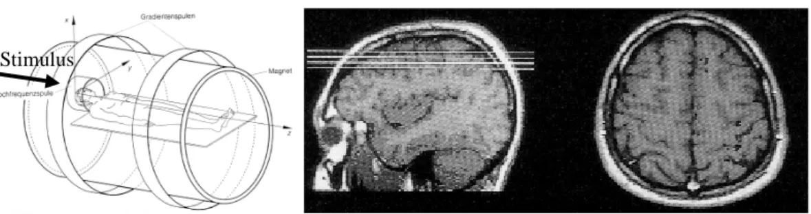
Functional magnetic resonance imaging (fMRI) is a non-invasive method to get insight into the function-ing of the brain. Sensory activation can be traced by the hemodynamic response to neuronal activity. This response, the blood oxygen level dependent effect, is typically very small and strongly distorted by noise in the same order of magnitude as the signal itself. Prob-lems and proceedings of detecting such activated re-gions, hence the reproducible recognition of regions (volumes) with the expected response, are outlined in

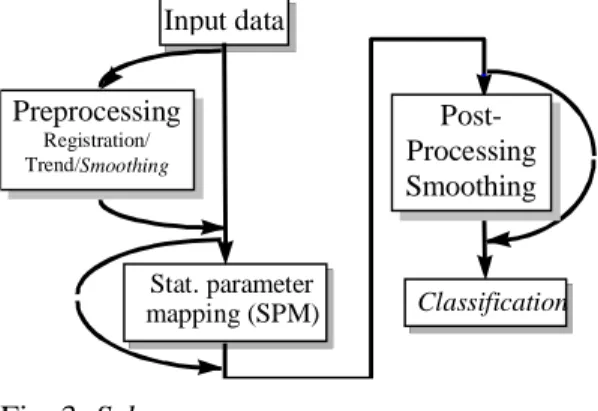
Fig. 1. A sketch of the BOLD-effect related to an activation is shown in Fig. 2. The distortion of the signals is the reason that activation patterns are re-peated to allow a better correlation to the response. From this noisy and distorted spatial-temporal signal the expected response has to be filtered out. Applied methods of signal processing base on non-linear con-cepts of data reconstruction and recently developed filters of mathematical morphology (e.g. alternating sequential morphological filters). The proceeding of data analysis is shown in Fig. 3.

Fig. 1. fMRI from the brain.

response BOLD Activation

time [ 3 sec]

Delay

Intensity

Input data

Stat. parameter

mapping (SPM) Classification Preprocessing Registration/ Trend/Smoothing Post-Processing Smoothing

Fig. 2. BOLD effect. Fig. 3. Scheme.

DATA ACQUISITION AND

MATERIAL

PHYSIOLOGY

Upon neuronal activation, oxygen consumption, blood flow and volume locally increase to meet the higher metabolic demand of neuronal tissue. The rise in blood flow is disproportionally larger than the oxy-gen consumption, probably due to limited oxyoxy-gen transport across capillaries. This results in a net in-crease in capillary and venous blood oxygenation, that can be measured by a special MR method, the so-called BOLD (blood oxygenation level dependent, Ogawa et al., 1990) technique. BOLD contrast is generated by susceptibility or T2* - sensitive sequences that exploit the different magnetic properties of deoxy-hemoglobin (DeoxHb, paramagnetic) and oxyhemo-globin (OxHb, diamagnetic), in that a reciprocal rela-tionship exists between concentration of DeoxHb and observed signal intensity. Local signal increase of BOLD-fMRI in response to a neuronal stimulus there-fore, reflects a rise in the OxHb to DeoxHb ratio and represents a non-invasive, yet indirect measure of neuronal activity.

fMRI was performed on a 1.5T Signa Echospeed (GE Medical Systems, Milwaukee) clinical scanner using the standard quadrature head coil. Multi-slice (7) single-shot gradient-echo echoplanar images (TR = 3000 ms, TE = 60 ms, flip angle = 90°) were acquired from the visual cortex during the visual stimulation period. Three on and four off periods (10 images each) were collected resulting in a time-series of 70 images and a temporal resolution of 3s. Nominal spatial resolution was 2.9×2.9×5 mm.

The visual stimulation was triggered with the MR acquisition and consisted of an 4 Hz alternating

checkerboard projected onto a screen in front of the magnet bore that could be viewed by the subject through a mirror system.

Data processing: To compensate motion artefacts, images were rigidly realigned using the AIR algorithm (Woods et al., 1998, AIR 3.08).

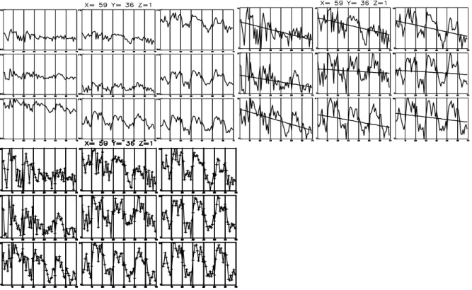
The pattern of stimuli is outlined in Fig. 2. Re-sponse signals in a 3×3×1 neighbourhood are dis-played in Fig. 4 (top left). After subtraction of the estimated linear trend (Fig. 4 top right), the resulting signals are outlined in Fig. 4 (lower left). The pre-sented data stem from a visual experiment, however the method presented is applicable to any activation type.

FUNCTIONAL MAPS

To calculate functional maps, a segmentation of activated from non-activated areas is performed on the basis of the time course of signal intensity, applying various statistical methods. Commonly, split t-test, cross-correlation to an ideal reference waveform or Fourier analysis are used to pixelwise map statistical values. The next step is to define an appropriate cut-off and superimpose only thresholded pixels on a high resolution anatomical MRI, thus producing the ‘func-tional map’.

Fig. 4. Data example, time signals in a 3×3×1 neighbourhood with trend elimination.

METHODS

NON-LINEAR GAUSSIAN FILTER AND

FILTER CHAINS

The filter used is known as sigma filter. The noisy function is convoluted by the product of two Gaussian functions weighting the spatial and intensity spread.

( )

(

)

(

( ) ( )

)

( )

NLG

, f p N_{q p}g q p g f q f p f q

σ ζ = _≈∑ σ − ζ −

1

with _g ( )_t t

λ = − _λ         exp 2 2 2 and

(

)

(

( ) ( )

)

N

g

q

p g

f q

f p

q

=

∑

−

−

normali-sation purposes.

The sequential application of this filter:

( )

faus = NLGσ ζ_k,_k

o o

with increasing spatial width (σ) and decreasing inten-sity width (ζ)

1 1

1 1

voxel width; and

1

3 of intensities e.g. 2

j j

j j

STD ; ;

σ

σ

α σ

ζ

ζ

ζ

α

α

+

= = ⋅

= ⋅ = =

is the so-called Aurich chain, see (Aurich, 1998; Win-kler et al., 1999).

SEQUENTIAL ALTERNATING FILTERS

FROM OPENINGS AND CLOSINGS IN

MATHEMATICAL MORPHOLOGY

With

A B

,

⊂

Ζ

;

0

∈

B

Dilation:

C

A

B

A

A

val B

b B b b B

= ⊕ =

=

+

( )

(

( ))

U

U

C

=

A

=

(

A B

)

⊕

B

Openclose:

C

=

(

A

)

are shortly and not exactly defined (see for complete descriptions Serra, 1986; Sternberg, 1986; Heijmans, 1995). The complementary functions like erosion,

closing and closeopen are defined accordingly. A

separate class of filters are the alternating sequential

morphological filter:

C AB B B B B

B B B B n n n

=(((...( 1) ) ) )...) ) ⊂ ⊂ ⊂...

1 2

2 ; 1 2

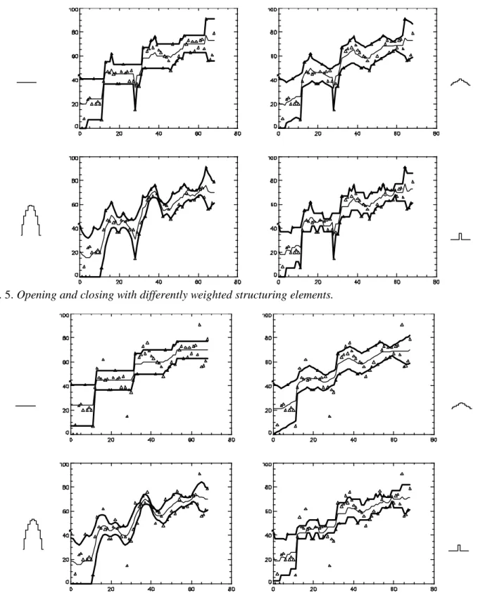
The application of filters from the field of mathe-matical morphology on discrete time functions is shown in Fig. 5, 6 for different structuring elements with differing weighting functions. The structuring elements with their weights in the time domain are displayed beside the graphs. Two thick plotted lines

show the filter results. The thin line represents the mean of the two complementary filters. This illustrates the behaviour of these filters on functions which is not widely used. Fig. 5 shows opening and closing with differently weighted structuring elements and Fig. 6 the results of openclose and closeopen.

Fig. 5. Opening and closing with differently weighted structuring elements.

TEST SCHEME FOR CLASSIFICATION

To evaluate or compare the filter results a classi-fier is implemented to test the existence of the activa-tion pattern by several minimum maximum compari-sons at certain adequate time intervals. This simple classifier does not replace an in-depth analysis using SPM or other tools for statistical analysis and dis-crimination. Its only purpose is to detect possible acti-vation and to illustrate filter results.

EXAMPLES

Several filters and filter configurations are tested with varying parameters. Depending on the models applied (defined by the filter or structuring element sizes and shapes) the results are considerably control-lable. This can be recognised in filter results shown in Fig. 5 and Fig. 6. The actually filtered signals used for classification could not be displayed due to the limited space.

NON-LINEAR GAUSSIAN FILTER AND

FILTER CHAIN

In Fig. 7 one section is shown with classification results for increasing spread of the spatial Gaussian. The increased spread σ of the Gaussian stabilise the

activation and reduces for higher spread the detection of artefacts.

SEQUENTIAL ALTERNATING FILTERS

Fig. 8 shows similar to Fig. 7 the classification re-sults for increasing spatial sizes of the structuring element with flat (unweighted) kernel in temporal di-mension.

SUMMARY AND DISCUSSION

The application and test of spatio-temporal filters is, beside the problems concerning the necessary com-puting time, not trivial. The response as well as the distortions of the data are influenced by many differ-ent sources. The two approaches can roughly be char-acterised like follows:

NON-LINEAR GAUSSIAN FILTER AND

FILTER CHAIN

- Modelling based on assumptions about the noise,

less a priori knowledge for data necessary/ possible

- Model often very simple (e.g. piece-wise constant function for the Aurich chain)

- Scaleability very good

Relatively high amount of computing time

Fig. 7. Classification of Aurich chain transformed sections with σ = 1, 2, 4.

MATHEMATICAL MORPHOLOGY

- Modelling of the data, more a priori knowledge for data necessary

- Modelling by set oriented methods arbitrarily

complicated

- Relatively little amount of computing time

The choice of method depends on the amount of knowledge available. Pre-processing can improve results of elaborated post-processing steps, e.g. SPM (statistical parameter mapping), considerably. However an objective evaluation of the methods is very difficult because of the number of unknown variants, the miss-ing knowledge about the noise function(s), but also by the lack of adequate representation methods for visuali-sation of higher dimensional (> 2) data.

A preliminary report of some of the data was presented at the Xth International Congress for Stereology, Melbourne, Australia, 1-4 November 1999.

REFERENCES

Aurich V, Mühlhaus E, Grundmann S (1998). Kantener-haltende Glättung von Volumendaten bei sehr ger-ingem Signal-Rausch-Verhältnis. 2. Aachener Work-shop über Bildverarbeitung in der Medizin.

Serra J (1982). Image Analysis and Mathematical Mor-phology. London: Academic Press.

Sternberg SR (1986). Grayscale Morphology, Computer Vision. Graphics and Image Processing 33:333-55. Heijmans HJAM (1995). Mathematical Morphology:

Ba-sic Principles. Summer School, Zakopane, Poland. Ogawa S, Lee TM, Kay AR (1990). Tank. Proc Natl Acad

Sci USA 87:9868-72.

Woods RP (1998). JCAT 22:155-65.