HAL Id: hal-01338330
https://hal.archives-ouvertes.fr/hal-01338330v4
Submitted on 8 Aug 2019HAL is a multi-disciplinary open access archive for the deposit and dissemination of sci-entific research documents, whether they are pub-lished or not. The documents may come from teaching and research institutions in France or abroad, or from public or private research centers.
L’archive ouverte pluridisciplinaire HAL, est destinée au dépôt et à la diffusion de documents scientifiques de niveau recherche, publiés ou non, émanant des établissements d’enseignement et de recherche français ou étrangers, des laboratoires publics ou privés.
The Jacobi Stochastic Volatility Model
Damir Filipovic, Damien Ackerer, Sergio Pulido
To cite this version:
Damir Filipovic, Damien Ackerer, Sergio Pulido. The Jacobi Stochastic Volatility Model. Finance and Stochastics, Springer Verlag (Germany), 2018, 22 (3), pp.667-700. �10.1007/s00780-018-0364-8�. �hal-01338330v4�
The Jacobi Stochastic Volatility Model
∗Damien Ackerer† Damir Filipovi´c‡ Sergio Pulido§
February 20, 2018
forthcoming in Finance and Stochastics
Abstract
We introduce a novel stochastic volatility model where the squared volatility of the asset return follows a Jacobi process. It contains the Heston model as a limit case. We show that the joint density of any finite sequence of log returns admits a Gram–Charlier A expansion with closed-form coefficients. We derive closed-form series representations for option prices whose discounted payoffs are functions of the asset price trajectory at finitely many time points. This includes European call, put, and digital options, forward start options, and can be applied to discretely monitored Asian options. In a numerical analysis we show that option prices can be accurately and efficiently approximated by truncating their series representations.
Keywords: Jacobi process, option pricing, polynomial model, stochastic volatility
MSC (2010): 91B25, 91B70, 91G20, 91G60
JEL Classification: C32, G12, G13
∗We thank the participants at the 2014 Stochastic Analysis in Finance and Insurance Conference in Oberwolfach, the
2015 AMaMeF and Swissquote Conference in Lausanne, the 2016 ICMS Workshop in Edinburgh, and the seminar at Mannheim Mathematics Department, as well as Stefano De Marco, Julien Hugonnier, Wahid Khosrawi-Sardroudi, Martin Larsson, and Peter Tankov for their comments. We thank an anonymous referee, an anonymous associate editor, and Chris Rogers (co-editor) for their careful reading of the manuscript and suggestions. The research leading to these results has received funding from the European Research Council under the European Union’s Seventh Framework Programme (FP/2007-2013) ERC Grant Agreement n. 307465-POLYTE. The research of Sergio Pulido benefited from the support of the Chair Markets in Transition (F´ed´eration Bancaire Fran¸caise) and the project ANR 11-LABX-0019.
†Swissquote Bank, Gland, Switzerland. E-mail: [email protected]
‡EPFL and Swiss Finance Institute, Lausanne, Switzerland. E-mail: [email protected]
§Laboratoire de Math´ematiques et Mod´elisation d’ ´Evry (LaMME), Universit´e d’ ´Evry-Val-d’Essonne, ENSIIE,
Uni-versit´e Paris-Saclay, ´Evry, France. E-mail: [email protected]
1
Introduction
Stochastic volatility models for asset returns are popular among practitioners and academics because they can generate implied volatility surfaces that match option price data to a great extent. They resolve the shortcomings of the Black–Scholes model [12], where the return has constant volatility. Among the the most widely used stochastic volatility models is the Heston model [33], where the squared volatility of the return follows an affine square-root diffusion. European call and put option prices in the Heston model can be computed using Fourier transform techniques, which have their numerical strengths and limitations; see for instance Carr and Madan [15], Bakshi and Madan [9], Duffie et al. [23], Fang and Oosterlee [28], and Chen and Joslin [16].
In this paper we introduce a novel stochastic volatility model, henceforth the Jacobi model, where the squared volatility Vt of the log price Xt follows a Jacobi process with values in some compact
interval [vmin, vmax]. As a consequence, Black–Scholes implied volatilities are bounded from below
and above by √vmin and √vmax. The Jacobi model (Vt, Xt) belongs to the class of polynomial
diffusions studied in Eriksson and Pistorius [26], Cuchiero et al. [19], and Filipovi´c and Larsson [30]. It includes the Black–Scholes model as a special case and converges weakly in the path space to the Heston model for vmax→ ∞ and vmin= 0.
We show that the log priceXT has a densitygthat admits a Gram–Charlier A series expansion with
respect to any Gaussian density w with sufficiently large variance. More specifically, the likelihood ratio function `=g/w lies in the weighted spaceL2
w of square-integrable functions with respect tow.
Hence it can be expanded as a generalized Fourier series with respect to the corresponding orthonormal basis of Hermite polynomialsHn(X0), n≥0. Boundedness ofVt is essential, as the Gram–Charlier A
series of gdoes not converge for the Heston model.
The Fourier coefficients `n of `are given by the Hermite moments of XT, `n =E[Hn(XT)]. Due
to the polynomial property of (Vt, Xt) the Hermite moments admit easy to compute closed-form
expressions. This renders the Jacobi model extremely useful for option pricing. Indeed, the price
πf of a European option with discounted payoff f(XT) for some function f in L2w is given by the
L2w-scalar product πf = (f, `)w=Pn≥0fn`n. The Fourier coefficientsfnoff are given in closed-form
for many important examples, including European call, put, and digital options. We approximateπf
by truncating the price series at some finite order N and derive truncation error bounds.
We extend our approach to price exotic options whose discounted payoff f(Y) depends on a fi-nite sequence of log returns Yi = (Xti −Xti−1),1 ≤ i≤ d. As in the univariate case we derive the
Gram–Charlier A series expansion of the densitygofY with respect to a properly chosen multivariate Gaussian densityw. Assuming that f lies in L2w the option price πf is obtained as a series
represen-tation of the L2w-scalar product in terms of the Fourier coefficients of f and of the likelihood ratio function`=g/w given by the corresponding Hermite moments ofY. Due to the polynomial property of (Vt, Xt) the Hermite moments admit closed-form expressions, which can be efficiently computed.
The Fourier coefficients of f are given in closed-form for various examples, including forward start options and forward start options on the underlying return.
Consequently, the pricing of these options is extremely efficient and does not require any numerical integration. Even when the Fourier coefficients of the discounted payoff function f are not available in closed-form, e.g. for Asian options, prices can be approximated by integratingf with respect to the Gram–Charlier A density approximation of g. This boils down to a numerically feasible integration with respect to the underlying Gaussian density w. In a numerical analysis we find that the price approximations become accurate within short CPU time. This is in contrast to the Heston model, for which the pricing of exotic options using Fourier transform techniques is cumbersome and creates numerical difficulties as reported in Kruse and N¨ogel [42], Kahl and J¨ackel [39], and Albrecher et al. [6]. In view of this, the Jacobi model also provides a viable alternative to approximate option prices in the Heston model.
The Jacobi process, also known as Wright–Fisher diffusion, was originally used to model gene frequencies; see for instance Karlin and Taylor [41] and Ethier and Kurtz [27]. More recently, the Jacobi process has also been used to model financial factors. For example, Delbaen and Shirakawa [20] model interest rates by the Jacobi process and study moment-based techniques for pricing bonds. In their framework, bond prices admit a series representation in terms of Jacobi polynomials. These
polynomials constitute an orthonormal basis of eigenfunctions of the infinitesimal generator and the stationary beta distribution of the Jacobi process; additional properties of the Jacobi process can be found in Mazet [47] and Demni and Zani [21]. The multivariate Jacobi process has been studied in Gourieroux and Jasiak [32] where the authors suggest it to model smooth regime shifts and give an example of stochastic volatility model without leverage effect. The Jacobi process has been also applied recently to model stochastic correlation matrices in Ahdida and Alfonsi [3] and credit default swap indexes in Bernis and Scotti [10].
Density series expansion approaches to option pricing were pioneered by Jarrow and Rudd [38]. They propose expansions of option prices that can be interpreted as corrections to the pricing biases of the Black–Scholes formula. They study density expansions for the law of underlying prices, not the log returns, and express them in terms of cumulants. Evidently, since convergence cannot be guaranteed in general, their study is based on strong assumptions that imply convergence. In subsequent work, Corrado and Su [17] and Corrado and Su [18] study Gram–Charlier A expansions of 4th order for options on the S&P 500 index. These expansions contain skewness and kurtosis adjustments to option prices and implied volatility with respect to the Black–Scholes formula. The skewness and kurtosis correction terms, which depend on the cumulants of 3rd and 4th order, are estimated from data. Due to the instability of the estimation procedure, higher order expansions are not studied. Similar studies on the biases of the Black–Scholes formula using Gram–Charlier A expansions include Backus et al. [8] and Li and Melnikov [44]. More recently, Drimus et al. [22] and Necula et al. [48] study related expansions with Hermite polynomials. In order to guarantee the convergence of the Gram– Charlier A expansion for a general class of diffusions, Ait-Sahalia [4] develop a technique based on a suitable change of measure. As pointed out in Filipovi´c et al. [31], in the affine and polynomial settings this change of measure usually destroys the polynomial property and the ability to calculate moments efficiently. More recently a similar study has been carried out by Xiu [53]. Gram–Charlier A expansions, under a change of measure, are also mentioned in the work of Madan and Milne [46], and the subsequent studies of Longstaff [45], Abken et al. [1] and Brenner and Eom [13], where they use these moment expansions to test the martingale property with financial data and hence the validity of a given model.
Our paper is similar to Filipovi´c et al. [31] in that it provides a generic framework to perform density expansions using orthonormal polynomial basis in weightedL2 spaces for affine models. They show that a bilateral Gamma density weight works for the Heston model. However, that expansion is numerically more cumbersome than the Gram–Charlier A expansion because the orthonormal basis of polynomials has to be constructed using Gram–Schmidt orthogonalization. In a related paper Heston and Rossi [34] study polynomial expansions of prices in the Heston, Hull-White and Variance Gamma models using logistic weight functions.
The remainder of the paper is as follows. In Section 2we introduce the Jacobi stochastic volatility model. In Section3we derive European option prices based on the Gram–Charlier A series expansion. In Section 4 we extend this to the multivariate case, which forms the basis for exotic option pricing and contains the European options as special case. In Section5 we give some numerical examples. In Section 6 we conclude. In Appendix A we explain how to efficiently compute the Hermite moments. All proofs are collected in Appendix B.
2
Model specification
We study a stochastic volatility model where the squared volatility follows a Jacobi process. Fix some real parameters 0≤vmin< vmax, and define the quadratic function
Q(v) = (v−vmin)(vmax−v) (√vmax−√vmin)2
.
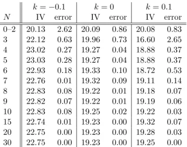
Inspection shows that v ≥ Q(v), with equality if and only if v = √vminvmax, and Q(v) ≥ 0 for all
v∈[vmin, vmax], see Figure 1for an illustration.
We consider the diffusion process (Vt, Xt) given by dVt=κ(θ−Vt)dt+σ p Q(Vt)dW1t dXt= (r−δ−Vt/2)dt+ρ p Q(Vt)dW1t+ p Vt−ρ2Q(Vt)dW2t (1)
for real parameters κ >0, θ ∈(vmin, vmax], σ >0, interest rate r, dividend yield δ, and ρ ∈[−1,1],
and where W1t and W2t are independent standard Brownian motions on some filtered probability
space (Ω,F,Ft,Q). The following theorem shows that (Vt, Xt) is well defined.
Theorem 2.1. For any deterministic initial state (V0, X0) ∈ [vmin, vmax]×R there exists a unique
solution (Vt, Xt) of (1) taking values in [vmin, vmax]×R and satisfying
Z ∞ 0
1{Vt=v}dt= 0 for all v∈[vmin, vmax). (2)
Moreover, Vt takes values in(vmin, vmax) if and only if V0 ∈(vmin, vmax) and
σ2(vmax−vmin)
(√vmax−√vmin)2 ≤
2κmin{vmax−θ, θ−vmin}. (3)
Remark 2.2. Property (2) implies that no state v ∈ [vmin, vmax) is absorbing. It also implies that conditional on{Vt, t∈[0, T]}, the incrementsXti−Xti−1 are non-degenerate Gaussian for anyti−1<
ti ≤T as will be shown in the proof of Theorem 4.1. Taking vmin = 0 and the limit as vmax → ∞, condition (3) coincides with the known condition that precludes the zero lower bound for the CIR process,σ2 ≤2κθ.
We specify the price of a traded asset bySt= eXt. Then√Vtis the stochastic volatility of the asset
return,dhX, Xit=Vtdt. The cumulative dividend discounted price process e−(r−δ)tStis a martingale.
In other words, Q is a risk-neutral measure. The parameter ρ tunes the instantaneous correlation
between the asset return and the squared volatility,
dhV, Xit p dhV, Vit p dhX, Xit =ρpQ(Vt)/Vt.
This correlation is equal to ρ if Vt =√vminvmax, see Figure1. In general, we have p
Q(Vt)/Vt ≤1.
Empirical evidences suggest that ρ is negative when St is a stock price or index. This is commonly
referred as the leverage effect, that is, an increase in volatility often goes along with a decrease in asset value.
Since the instantaneous squared volatility Vt follows a bounded Jacobi process on the interval
[vmin, vmax], we refer to (1) as the Jacobi model. For V0 = θ = vmax we have constant volatility
Vt=V0 for all t≥0 and we obtain the Black–Scholes model
dXt= (r−δ−V0/2)dt+ p
V0dW2t. (4)
For vmin = 0 and the limit vmax → ∞ we haveQ(v) →v, and we formally obtain the Heston model
as limit case of (1), dVt=κ(θ−Vt)dt+σ p VtdW1t dXt= (r−δ−Vt/2)dt+ p Vt ρ dW1t+ p (1−ρ2)dW 2t . (5)
In fact, the Jacobi model (1) is robust with respect to perturbations, or mis-specifications, of the model parametersvmin,vmax and initial state (V0, X0). Specifically, the following theorem shows that the diffusion (1) is weakly continuous in the space of continuous paths with respect tovmin,vmax and
(V0, X0). In particular, the Heston model (5) is indeed a limit case of our model (1).
Consider a sequence of parameters 0≤vmin(n) < vmax(n) and deterministic initial states (V0(n), X (n)
0 )∈
[v(minn) , vmax(n) ]×Rconverging to 0≤vmin < vmax≤ ∞and (V0, X0)∈[0,∞)×Rasn→ ∞, respectively.
We denote by (Vt(n), Xt(n)) and (Vt, Xt) the respective solutions of (1), or (5) ifvmax=∞. Here is our
Theorem 2.3. The sequence of diffusions (Vt(n), Xt(n)) converges weakly in the path space to (Vt, Xt) as n→ ∞.
As the discounted put option payoff functionfput(x) = e−rT(ek−ex)+ is bounded and continuous
on R, it follows from the weak continuity stated in Theorem 2.3that the put option prices based on
(Vt(n), Xt(n)) converge to the put option price based on the limiting model (Vt, Xt) as n → ∞. The
put-call parity, πcall−πput = e−δTS0−e−rT+k, then implies that also call option prices converge as
n→ ∞. This carries over to more complex path-dependent options with bounded continuous payoff functional.
Polynomial property
Moments in the Jacobi model (1) are given in closed-form. Indeed, let
Gf(v, x) =b(v)>∇f(v, x) +1
2Tr a(v)∇
2f(v, x)
denote the generator of (Vt, Xt) with drift vectorb(v) and the diffusion matrixa(v) given by
b(v) = κ(θ−v) r−δ−v/2 , a(v) = σ2Q(v) ρσQ(v) ρσQ(v) v . (6)
Observe that a(v) is continuous in the parametersvmin,vmax, so that forvmin = 0 andvmax→ ∞we
obtain a(v)→ σ2v ρσv ρσv v ,
which corresponds to the generator of the Heston model (5). Let Poln be the vector space of
polyno-mials in (v, x) of degree less than or equal to n. It then follows by inspection that the components of
b(v) and a(v) lie in Pol1 and Pol2, respectively. As a consequence, G maps any polynomial of degree
n onto a polynomial of degree n or less, GPoln ⊂ Poln, so that (Vt, Xt) is a polynomial diffusion,
see Filipovi´c and Larsson [30, Lemma 2.2]. From this we can easily calculate the conditional moments of (VT, XT) as follows. For N ∈ N, let M = (N + 2)(N + 1)/2 denote the dimension of PolN. Let
h1(v, x), . . . , hM(v, x) be a basis of polynomials of PolN and denote byGthe matrix representation of
the linear mapG restricted to PolN with respect to this basis.
Theorem 2.4. For any polynomial p∈PolN and0≤t≤T we have
Ep(VT, XT)
Ft= h1(Vt, Xt) · · · hM(Vt, Xt)e(T−t)G#»p
where #»p ∈ RM is the coordinate representation of the polynomial p(v, x) with respect to the basis h1(v, x), . . . , hM(v, x).
Proof. See Filipovi´c and Larsson [30, Theorem 3.1].
The moment formula in Theorem 2.4 is crucial in order to efficiently implement the numerical schemes described below.
3
European option pricing
Henceforth we assume that (V0, X0)∈[vmin, vmax]×R is a deterministic initial state and fix a finite
time horizon T > 0. We first establish some key properties of the distribution of XT. Denote the
quadratic variation of the second martingale component of Xt in (1) by
Ct= Z t 0 Vs−ρ2Q(Vs) ds. (7)
Theorem 3.1. Let <1/(2vmaxT). The distribution ofXT admits a densitygT(x)onRthat satisfies Z R ex2gT(x)dx <∞. (8) If E h CT−1/2−k i <∞ (9)
for some k∈ N0 then gT(x) and ex
2
gT(x) are uniformly bounded and gT(x) is k-times continuously differentiable on R. A sufficient condition for (9) to hold for any k≥0 is
vmin >0 and ρ2<1.1 (10)
The condition that < 1/(2vmaxT) is sharp for (8) to hold. Indeed, consider the Black–Scholes
model (4) whereVt=θ=vmax for allt≥0. ThenXT is Gaussian with varianceCT =vmaxT. Hence
the integral in (8) is infinite for any ≥1/(2vmaxT).
Since any uniformly bounded and integrable function onRis square integrable on R, as an
imme-diate consequence of Theorem3.1we have the following corollary. Corollary 3.2. Assume (9) holds for k= 0. Then
Z
R
gT(x)2
w(x) dx <∞ (11)
for any Gaussian density w(x) with variance σ2w satisfying
σw2 > vmaxT
2 . (12)
Remark 3.3. It follows from the proof that the statements of Theorem 3.1 also hold for the Heston model (5) with Q(v) = v and = 0. However, the Heston model does not satisfy (8) for any > 0. Indeed, otherwise its moment generating function
c
gT(z) = Z
R
ezxgT(x)dx (13)
would extend to an entire function in z ∈ C. But it is well known that gcT(z) becomes infinite for large enough z ∈ R, see Andersen and Piterbarg [7]. As a consequence, the Heston model does not
satisfy (11) for any finite σw. Indeed, by the Cauchy-Schwarz inequality, (11) implies (8) for any
<1/(4σ2w).
We now compute the price at time t = 0 of a European claim with discounted payoff f(XT) at
expiry date T >0. We henceforth assume that (9) holds with k= 0, and we let w(x) be a Gaussian density with meanµw and varianceσw2 satisfying (12). We define the weighted Lebesgue space
L2w= f(x) :kfk2w= Z R f(x)2w(x)dx <∞ ,
which is a Hilbert space with scalar product
(f, g)w= Z
R
f(x)g(x)w(x)dx.
The space L2w admits the orthonormal basis of generalized Hermite polynomialsHn(x), n≥0, given
by Hn(x) = 1 √ n!Hn x−µw σw (14) 1
We conjecture that (9) holds for anyk≥0 also whenvmin= 0 (andκθ >0) orρ2 = 1. For the Heston model (5)
whereHn(x) are the standard Hermite polynomials defined by Hn(x) = (−1)ne x2 2 d n dxne −x2 2 , (15)
see Feller [29, Section XVI.1]. In particular, the degree of Hn(x) is n, and (Hm, Hn)w = 1 if m =n
and zero otherwise.
Corollary 3.2implies that the likelihood ratio function `(x) =gT(x)/w(x) of the densitygT(x) of
the log priceXT with respect tow(x) belongs toL2w. We henceforth assume that also the discounted
payoff function f(x) is in L2
w. This hypothesis is satisfied for instance in the case of European call
and put options. It implies that the price, denoted by πf, is well defined and equals
πf = Z R f(x)gT(x)dx= (f, `)w = X n≥0 fn`n, (16)
for theFourier coefficients of f(x)
fn= (f, Hn)w, (17)
and the Fourier coefficients of`(x) that we refer to asHermite moments
`n= (`, Hn)w = Z
R
Hn(x)gT(x)dx. (18)
We approximate the priceπf by truncating the series in (16) at some order N ≥1 and write
πf(N) =
N X n=0
fn`n, (19)
so that πf(N) → πf as N → ∞. Due to the polynomial property of the Jacobi model, (19) induces
an efficient price approximation scheme because the Hermite moments `n are linear combinations of
moments of XT and thus given in closed-form, see Theorem 2.4. In particular, sinceH0(x) = 1, we have `0= 1. More details on the computation of `nare given in Appendix A.
With the Hermite moments `n available, the computation of the approximation (19) boils down
to a numerical integration, πf(N)= N X n=0 (f, `nHn)w= Z R f(x)`(N)(x)w(x)dx, (20)
of f(x)`(N)(x) with respect to the Gaussian distribution w(x)dx, where the polynomial `(N)(x) =
PN
n=0`nHn(x) is in closed-form. The integral (20) can be computed by quadrature or Monte-Carlo
simulation. In specific cases, we find closed-form formulas for the Fourier coefficients fn and no
numerical integration is needed. This includes European call, put, and digital options, as shown below.
Remark 3.4. Formula (20) shows that gT(N)(x) = `(N)(x)w(x) serves as an approximation for the density gT(x). In fact, we readily see that gT(N)(x) integrates to one and converges to gT(x) in L21/w as N → ∞. Hence, we have convergence of the Gram–Charlier A series expansion of the density of the log price XT in L21/w.2 In view of Remark 3.3, this does not hold for the Heston model.
Matching the first moment or the first two moments ofw(x) and gT(x), we further obtain
`1 = Z
R
H1(x)gT(x)dx= (H0, H1)w = 0 ifµw =E[XT],
2A Gram–Charlier A series expansion of a density functiong(x) is formally defined asg(x) =P
n≥0cnHn(x)w(x) for
and similarly,
`1 =`2= 0 ifµw =E[XT] and σw2 = var[XT]. (21)
Matching the first moment or the first two moments of w(x) and gT(x) can improve the convergence
of the approximation (19). Note however that (12) and (21) imply var[XT]> vmaxT /2, so that second
moment matching is not always feasible in empirical applications.
Remark 3.5. Ifµw =X0+(r−δ)T−σw2/2, thenf0=RRf(x)w(x)dxis the Black–Scholes option price
with volatility parameter σBS = σw/
√
T. Because E[XT] =X0+ (r−δ)T −var[XT]/2, this holds in particular if the first two moments of w(x) and gT(x) match, see (21). In this case, the higher order terms in π(fN)=f0+PNn=3fn`n can be thought of as corrections to the corresponding Black–Scholes pricef0 due to stochastic volatility.
The following result, which is a special case of Theorem 4.4 below, provides universal upper and lower bounds on the implied volatility of a European option with discounted payoff f(XT) at
T and price πf. The implied volatility σIV is defined as the volatility parameter that renders the corresponding Black–Scholes option price equal toπf.
Theorem 3.6. Assume that the discounted payoff function f(log(s)) is convex in s >0. Then the implied volatility satisfies √vmin ≤σIV ≤√vmax.
Examples
We now present examples of discounted payoff functions f(x) for which closed-form formulas for the Fourier coefficients fnexist. The first example is a call option.3
Theorem 3.7. Consider the discounted payoff function for a call option with log strikek,
f(x) = e−rTex−ek+. (22)
Its Fourier coefficients fn in (17) are given by
f0 = e−rT+µwI0 k−µw σw ;σw −e−rT+kΦ µw−k σw ; fn= e−rT+µw 1 √ n!σwIn−1 k−µw σw ;σw , n≥1. (23)
The functions In(µ;ν) are defined recursively by
I0(µ;ν) = e
ν2
2 Φ(ν−µ);
In(µ;ν) =Hn−1(µ)eνµφ(µ) +νIn−1(µ;ν), n≥1,
(24)
where Φ(x) denotes the standard Gaussian distribution function and φ(x) its density.
The Fourier coefficients of a put option can be obtained from the put-call parity. For digital options, the Fourier coefficients fn are as follows.
Theorem 3.8. Consider the discounted payoff function for a digital option of the form
f(x) = e−rT1[k,∞)(x).
Its Fourier coefficients fn are given by
f0= e−rTΦ µw−k σw ; fn= e−rT √ n!Hn−1 k−µw σw φ k−µw σw , n≥1, (25)
where Φ(x) denotes the standard Gaussian distribution function and φ(x) its density.
3
Similar recursive relations of the Fourier coefficients for the physicist Hermite polynomial basis can be found in Drimus et al. [22]. The physicist Hermite polynomial basis is the orthogonal polynomial basis of theL2
w space equipped
with the weight functionw(x) = e−x2 so that (Hn, Hn)w=
√
For a digital option with generic payoff 1[k1,k2)(x) the Fourier coefficients can be derived using Theorem3.8 and1[k1,k2)(x) =1[k1,∞)(x)−1[k2,∞)(x).
Error bounds and asymptotics
We first discuss an error bound of the price approximation scheme (19). The error of the approximation is(N) =π
f −π(fN)=P∞n=N+1fn`n for a fixed order N ≥1. The Cauchy–Schwarz inequality implies
the following error bound
|(N)| ≤ kfk2w− N X n=0 fn2 !1 2 k`k2w− N X n=0 `2n !1 2 . (26)
The L2w-norm of f(x) has an explicit expression, kfk2 w =
R
Rf(x)
2w(x)dx, that can be computed by quadrature or Monte–Carlo simulation. The Fourier coefficients fn can be computed similarly. The
Hermite moments`nare given in closed-form. It remains to compute theL2w-norm of`(x). For further
use we define Mt=X0+ Z t 0 (r−δ−Vs/2)ds+ ρ σ Vt−V0− Z t 0 κ(θ−Vs)ds , (27)
so that, in view of (1), the log priceXt=Mt+ Rt
0 p
Vs−ρ2Q(Vs)dW2s. Recall alsoCt given in (7).
Lemma 3.9. TheL2w-norm of `(x) is given by
k`k2w = Z R gT(x)2 w(x) dx=E gT(XT) w(XT) =E φ XT,MfT,CeT φ(XT, µw, σ2w) (28)
where φ(x, µ, σ2) is the normal density function in x with mean µ and variance σ2, and the pair of
random variables (MfT,CeT) is independent from XT and has the same distribution as (MT, CT).
In applications, we compute the right hand side of (28) by Monte–Carlo simulation of (XT,MfT,CeT)
and thus obtain the error bound (26).
We next show that the Hermite moments `n decay at an exponential rate under some technical
assumptions.
Lemma 3.10. Suppose that (10) holds and σw2 > vmaxT. Then there exist finite constantsC >0 and
0< q <1 such that`2n≤Cqn for alln≥0.
Comparison to Fourier transform
An alternative dual expression of the price πf in (16) is given by the Fourier integral
πf = 1 2π Z R ˆ f(−µ−iλ)ˆgT(µ+ iλ)dλ, (29)
where fb(z) and gcT(z) denote the moment generating functions given by (13), respectively. Here
µ ∈ R is some appropriate dampening parameter such that e−µxf(x) and eµxgT(x) are Lebesgue
integrable and square integrable on R. Indeed, Lebesgue integrability implies that fb(z) and gcT(z)
are well defined for z ∈ µ+ iR through (13). Square integrability and the Plancherel Theorem
then yield the representation (29). For example, for the European call option (22) we have fb(z) = e−rT+k(1+z)/(z(z+ 1)) for Re(z)<−1
Option pricing via (29) is the approach taken in the Heston model (5), for which there exists a closed-form expression for gcT(z). It is given in terms of the solution of a Riccati equation. The
computation ofπf boils down to the numerical integration of (29) along with the numerical solution
model (which entails vmax → ∞) does not adhere to the series representation (16) that is based on
condition (11), see Remark3.3.
The Jacobi model, on the other hand, does not admit a closed-form expression for gcT(z). But
the Hermite moments `n are readily available in closed-form. In conjunction with Theorem 3.7,
the (truncated) series representation (16) thus provides a valuable alternative to the (numerical) Fourier integral approach (29) for option pricing. Moreover, the approximation (20) can be applied to any discounted payoff function f(x) ∈ L2
w. This includes functions f(x) that do not necessarily
admit closed-form moment generating function fb(z) as is required in the Heston model approach. In Section 4, we further develop our approach to price path dependent options, which could be a cumbersome task using Fourier transform techniques in the Heston model.
4
Exotic option pricing
Pricing exotic options with stochastic volatility models is a challenging task. We show that the price of an exotic option whose payoff is a function of a finite sequence of log returns admits a polynomial series representation in the Jacobi model.
Henceforth we assume that (V0, X0) ∈ [vmin, vmax]×R is a deterministic initial state. Consider
time points 0 =t0 < t1 < t2 <· · ·< td and denote the log returns Yti =Xti −Xti−1 fori= 1, . . . , d.
The following theorem contains Theorem 3.1as special case whered= 1.
Theorem 4.1. Let 1, . . . , d∈R be such thati <1/(2vmax(ti−ti−1)) for i= 1, . . . , d. The random
vector (Yt1, . . . , Ytd) admits a densitygt1,...,td(y) on R
d satisfying Z Rd ePdi=1iyi2gt 1,...,td(y)dy <∞. If E " d Y i=1 (Cti−Cti−1) −1/2−ni # <∞ (30)
for all(n1. . . , nd)∈Nd0with Pd
i=1ni ≤k∈N0, for somek∈N0, thengt1,...,td(y)ande
Pd
i=1iy2igt
1,...,td(y)
are uniformly bounded and gt1,...,td(y) isk-times continuously differentiable on R
d. Property (10) im-plies (30) for anyk≥0.
Since any uniformly bounded and integrable function on Rd is square integrable on Rd, as an
immediate consequence of Theorem4.1 we have the following corollary. Corollary 4.2. Assume (30) holds for k= 0. Then
Z Rd gt1,...,td(y)2 Qd i=1wi(yi) dy <∞
for all Gaussian densities wi(yi) with variances σw2i satisfying
σw2i > vmax(ti−ti−1)
2 , i= 1, . . . , d. (31) Remark 4.3. There is a one-to-one correspondence between the vector of log returns (Yt1, . . . , Ytd)
and the vector of log prices (Xt1, . . . , Xtd). Indeed,
Xti =X0+
i X j=1
Ytj.
Hence, a crucial consequence of Theorem 4.1 is that the finite-dimensional distributions of the pro-cess Xt admit densities with nice decay properties. More precisely, the density of (Xt1, . . . , Xtd) is
Suppose that the discounted payoff of an exotic option is of the form f(Xt1, ..., Xtd). Assume
that (30) holds with k = 0. Set the weight function w(y) =Qdi=1wi(yi), where wi(y) is a Gaussian
density with meanµwi and varianceσ2wi satisfying (31). Define
e
f(y) =f(X0+y1, X0+y1+y2, . . . , X0+y1+· · ·+yd).
Then by similar arguments as in Section3 the price of the option is
πf =E[f(Xt1, ..., Xtd)] =
X n1,...,nd≥0
e
fn1,...,nd`n1,...,nd
where the Fourier coefficientsfen1,...,nd and the Hermite moments `n1,...,nd are given by
e fn1,...,nd = (f , He n1,...,nd)w = Z Rd e f(y)Hn1,...,nd(y)w(y)dy and `n1,...,nd =E Hn1,...,nd(Yt1, . . . , Ytd) (32) with Hn1,...,nd(y1, . . . , yd) = Qd i=1H (i) ni(yi), where H (i)
ni(yi) is the generalized Hermite polynomial of
degree ni associated to parameters µwi and σwi, see (14). The price approximation at truncation
order N ≥1 is given, in analogy to (19), by
πf(N)= N X n1+···+nd=0 e fn1,...,nd`n1,...,nd, (33) so that π(fN)→πf asN → ∞.
We now derive universal upper and lower bounds on the implied volatility for the exotic option with discounted payoff functionf(Xt1, ..., Xtd) and price πf. We denote by
dStBS=StBS(r−δ)dt+StBSσBSdBt (34)
the Black–Scholes price process with volatility σBS > 0 where Bt is some Brownian motion. The
Black–Scholes price is defined by
πσIV
f =E
h
f logStBS1 , . . . ,logStBSd i.
The implied volatilityσIV is the volatility parameterσBS that renders the Black–Scholes option price
πσIV
f =πf. The following theorem provides bounds on the values that σIV may take.
Theorem 4.4. Assume that the payoff functionf(log(s1), . . . ,log(sd))is convex in the prices(s1, . . . , sd)∈
(0,∞)d. Then the implied volatility satisfies √vmin ≤σIV≤√vmax.
Examples
We provide some examples of exotic options on the asset with price St = eXt for which our method
applies.
The payoff of aforward start call option on the underlying returnbetween datestandT, and with strike K is (ST/St−K)+ and its discounted payoff function is given by
e
f(y) = e−rT(ey2 −K)+
with the times t1 =t and t2 =T. Note that fe(y) = fe(y2) only depends on y2, so that this example reduces to the univariate case. In particular, the Fourier coefficients ˜fn coincide with those of a call
option and, as we shall see in Theroem A.3, the forward Hermite moments `∗n = E[Hn(Xt2 −Xt1)]
can be computed efficiently. Theorem4.4applies in particular to the forward start call option on the underlying return, so that its implied volatility is uniformly bounded for all maturities T > t. On
the other hand, we know from Jacquier and Roome [37] that in the Heston model the same implied volatility explodes (except at the money) when T →t.
The payoff of a forward start call option with maturity T, strike fixing date t and proportional strike K is (ST −KSt)+ and its discounted payoff function is given by
e
f(y) = e−rT eX0+y1+y2 −KeX0+y1+
with the timest1 =tand t2 =T. In this case the Fourier coefficients have the form ˜ fn1,n2 = e X0−rT Z R2 ey1H n1(y1)w1(y1)(e y2 −K)+H n2(y2)w2(y2)dy1dy2 = eX0−rTf(0,−∞) n1 f (0,logK) n2 =f (0,logK) n2 σn1 w √ n1! eX0−rT+µw1+σ2w1/2,
wherefn(r,k)denotes the Fourier coefficient of a call option for interest raterand log strikekas in (23).
Here we have used (23)–(24) to deduce that fn(01,−∞) =
σn1 w
√
n1!e
µw1+σ2w1/2. In particular no numerical
integration is needed. Additionally, the Hermite moments
`n1,n2 =E
Hn1(Yt1)Hn2(Yt2)
can be calculated efficiently as explained in Theorem A.3. The pricing of forward start call options (on the underlying return) in the Black–Scholes model is straightforward. Analytical expressions for forward start call options (on the underlying return) have been provided in the Heston model by Kruse and N¨ogel [42]. However, these integral expressions involve the Bessel function of first kind and are therefore rather difficult to implement numerically.
The payoff of an Asian call option with maturity T, discrete monitoring dates t1 <· · ·< td=T,
and fixed strikeK is (Pdi=1Sti/d−K)+ and its discounted payoff function is given by
e f(y) = e−rT 1 d d X i=1 eX0+Pij=1yi−K !+ .
The payoff of an Asian call option with floating strike is (ST −KPdi=1Sti/d)
+ and its discounted payoff function is given by
e f(y) = e−rT eX0+Pdj=1yj −K d d X i=1 eX0+Pij=1yj !+ .
The valuation of Asian options with continuously monitoring in the Black–Scholes model has been studied in Rogers and Shi [51] and Yor [55] among others.
Remark 4.5. The Fourier coefficients may not be available in closed-form for some exotic options, such as the Asian options. In this case, we compute the multi-dimensional version of the approximation
(19) via numerical integration of (20) with respect to a Gaussian density w(x) in Rd. This can be
efficiently implemented using Gauss-Hermite quadrature, see for example J¨ackel [36]. Specifically, denote zm ∈ Rd and wm ∈ (0,1) the m-th point and weight of an d-dimensional standard Gaussian cubature rule with M points. The price approximation can then be computed as follows
πf(N)= Z Rd ˜ f µ+ Σz`(N) µ+ Σz 1 (2π)d2 e−kzk 2 2 dz ≈ M X m=1 wmf˜m X n1+···+nd≤N `n1,...,nd d Y i=1 1 √ ni!Hni (zm,i) (35) where µ = (µw1, . . . , µwd) >, Σ = diag(σ
w1, . . . , σwd), f˜m = ˜f(µ+ Σzm), and Hn denotes the
stan-dard Hermite polynomial (15). We emphasize that many elements in the above expression can be precomputed. A numerical example is given for the Asian option in Section 5.2 below.
5
Numerical analysis
We analyse the performance of the price approximation (19) with closed-form Fourier coefficients and numerical integration of (20) for European call options, forward start and Asian options. This includes price approximation error, model implied volatility, and computational time. The model parameters are fixed as: r=δ =X0= 0,κ= 0.5,θ=V0 = 0.04,vmin= 10−4,vmax= 0.08,ρ=−0.5, andσ = 1.
The parameter values are in line with what could be obtained from a calibration to market prices, such as S&P500 option prices, with the exception of vmax that is set smaller than the typical fitted
value. The choice vmax = 0.08 permits to match the first two moments of w(x) and g(x) as in (21),
which improves the convergence of the approximation (19). We refer to Ackerer and Filipovi´c [2] for an extension of the polynomial option pricing method, which works well for arbitrary parameter values.
5.1 European call option
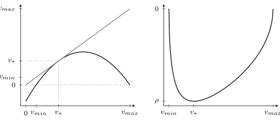
Figure 2displays Hermite moments `n, Fourier coefficients fn, and approximation option prices πf(N)
for a European call option with maturity T = 1/12 and log strike k = 0 (ATM) as functions of the truncation order N. The first two moments of the Gaussian density w(x) match the first two moments of XT, see (21).4 We observe that the `n and fn sequences oscillate and converge toward
zero. The amplitudes of these oscillations negatively impact the speed at which the approximation price sequence converges. The gray lines surrounding the price sequence are the upper and lower price error bounds computed as in (26) and Lemma 3.9, using 105 Monte-Carlo samples. The price approximation converges rapidly.
Table 1 reports the implied volatility values and absolute errors in percentage points for the log strikes k = {−0.1,0,0.1} and for various truncation orders. The reference option prices have been computed at truncation order N = 50. For all strikes the truncation order N = 10 is sufficient to be within 10 basis points of the reference implied volatility.
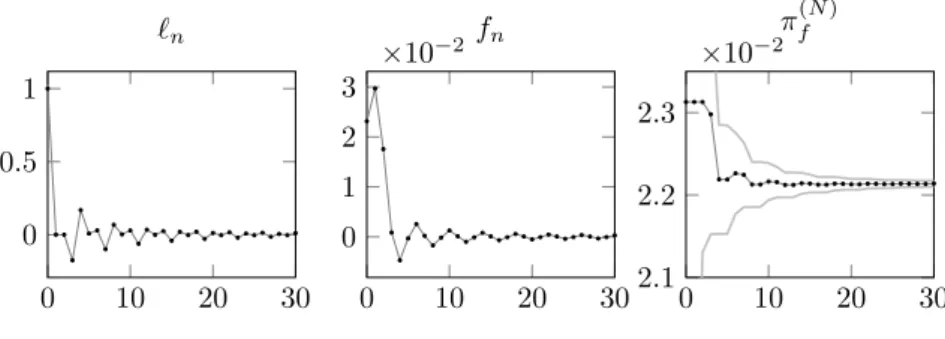
Figure 3displays the implied volatility smile for variousvmin and vmax such that√vminvmax =θ,
and for the Heston model (5). We observe that the smile of the Jacobi model approaches the Heston smile whenvmin is small and vmax is large. Somewhat surprisingly, a relatively small value for vmax
seems to be sufficient for the two smiles to coincide for options around the money. Indeed, although the variance process has an unbounded support in the Heston model, the probability that it will visit values beyond some large threshold can be extremely small. Figure3 also illustrates how the implied volatility smile flattens when the variance support shrinks,vmax↓θ. In the limitvmax =θ, we obtain
the flat implied volatility smile of the Black–Scholes model. This shows that the Jacobi model lies between the Black–Scholes model and the Heston model and that the parametersvmin and vmaxoffer
additional degrees of flexibility to model the volatility surface.
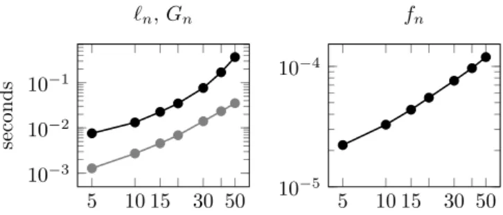
As reported in Figure 4, the Fourier coefficients can be computed in less than a millisecond thanks to the recursive scheme (23)-(24). Computing the Hermite moments is more costly, however they can be used to price all options with the same maturity. The most expensive task appears to be the construction of the matrix G, which however is a one-off. The Hermite moment `n in turn derives
from the vectorvn,T = eGTeπ(0,n) which can be used for any initial state (V0, X0). Note that specific numerical methods have been developed to compute the action of the matrix exponential eGT on the basis vector eπ(0,n), see for example Al-Mohy and Higham [5], Hochbruck and Lubich [35], and references therein. The running times were realized with a standard desktop computer using a single 3.5 Ghz 64 bits CPU and theRprogramming language.
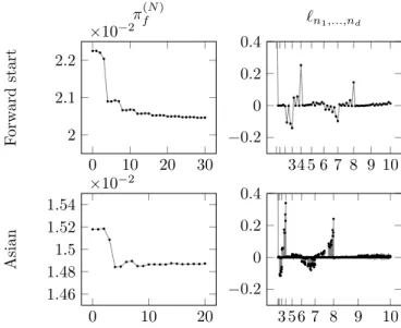
5.2 Forward start and Asian options
The left panels of Figure5 display the approximation prices of a forward start call option with strike fixing time t1 = 1/52 and maturity t2 = 5/52, so that d = 2, and of an Asian call option with weekly discrete monitoring and maturity four weeks, ti =i/52 for i≤d= 4. Both options have log
strike k= 0. The price approximations at orderN have been computed using (33). For the forward
4
In practice, depending on the model parameters, this may not always be feasible, in which case the truncation order N should be increased.
start call option, we match the first two moments of wi(yi) and Yti. For the Asian call option, we
chose σwi =
p
vmax/104 + 10−4 and µwi = E[X1/52], which is in line with (31) but does not match
the first two moments of Yti. The Fourier coefficients are not available in closed-form for the Asian
call option, therefore we integrated its payoff function with respect to the density approximation using Gaussian cubature as described in Remark 4.5. We observe that with exotic payoffs the price approximation sequence may require a larger order before stabilizing. For example, for the forward start price approximation it seems necessary to truncate beyondN = 15 in order to obtain a accurate price approximation.
The Asian option price is approximated by (35) whose computational cost depends on the number of elements in the double summation. Therefore, in order to efficiently approximate the price, we used a truncation of the 4-dimensional product of the one-dimensional Gaussian quadrature with 20 points. More precisely, we selected the quadrature points having a weight larger than the 90% quantile of all the weights. This means that, out of the 204 initial points, M = 16 000 points were selected and their weights normalized. Note that the 144 000 removed points had a total weight of 7.2×10⁻⁴ percent which is extremely small. Hence, the selected points cover most of the non-negligible part of the multivariate Gaussian density support. An alternative approach would be to use optimal Gaussian quantizers, see Pag`es and Printems [49].
The right panels of Figure 5 display the multi-index Hermite moments `n1,...,nd with multi-orders
n1+· · ·+nd= 1, . . . ,10. Note that there are NN+d
Hermite moments`n1,...,nd of total ordern1+· · ·+
nd ≤ N. In practice, we observe that a significant proportion of the Hermite moments is negligible
so that they may simply be set to zero if they are smaller than a certain threshold to be computed online. As for the quadrature points, doing so reduces the computational cost of approximating the option price. Therefore, when approximating the Asian option price, we removed the Hermite moments having an absolute value smaller than the correspondning 10% quantile. For example, when
N = 20, this implies removing all the Hermite moments with an absolute value|`n1,...,nd|smaller than
2.35×10⁻⁶.
6
Conclusion
The Jacobi model is a highly tractable and versatile stochastic volatility model. It contains the Heston stochastic volatility model as a limit case. The moments of the finite dimensional distributions of the log prices can be calculated explicitly thanks to the polynomial property of the model. As a result, the series approximation techniques based on the Gram–Charlier A expansions of the joint distributions of finite sequences of log returns allow us to efficiently compute prices of options whose payoff depends on the underlying asset price at finitely many time points. Compared to the Heston model, the Jacobi model offers additional flexibility to fit a large range of Black–Scholes implied volatility surfaces. Our numerical analysis shows that the series approximations of European call, put and digital option prices in the Jacobi model are computationally comparable to the widely used Fourier transform techniques for option pricing in the Heston model. The truncated series of prices, whose computations do not require any numerical integration, can be implemented efficiently and reliably up to orders that guarantee accurate approximations as shown by our numerical analysis. The pricing of forward start options, which does not involve any numerical integration, is significantly simpler and faster than the iterative numerical integration method used in the Heston model. The minimal and maximal volatility parameters are universal bounds for Black–Scholes implied volatilities and provide additional stability to the model. In particular, Black–Scholes implied volatilities of forward start options in the Jacobi model do not experience the explosions observed in the Heston model. Furthermore, our density approximation technique in the Jacobi model circumvents some limitations of the Fourier transform techniques in affine models and allows us to price discretely monitored Asian options.
A
Hermite moments
We apply Theorem 2.4 to describe more explicitly how the Hermite moments `0, . . . , `N in (18) can
{1, . . . , M} be an enumeration of the set of exponents
E ={(m, n) :m, n≥0;m+n≤N}.
The polynomials
hπ(m,n)(v, x) =vmHn(x), (m, n)∈ E (36)
then form a basis of PolN. In view of the elementary property
Hn0(x) = √
n σw
Hn−1(x), n≥1,
we obtain that theM×M–matrixGrepresentingGon PolN has at most 7 nonzero elements in column
π(m, n) with (m, n)∈ E given by Gπ(m−2,n),π(m,n)=− σ2m(m−1)vmaxvmin 2(√vmax−√vmin)2 , m≥2; Gπ(m−1,n−1),π(m,n)=− σρm√nvmaxvmin σw(√vmax−√vmin)2 , m, n≥1; Gπ(m−1,n),π(m,n)=κθm+ σ2m(m−1)(vmax+vmin) 2(√vmax−√vmin)2 , m≥1; Gπ(m,n−1),π(m,n)= (r−δ)√n σw +σρm √ n(vmax+vmin) σw(√vmax−√vmin)2 , n≥1; Gπ(m+1,n−2),π(m,n)= p n(n−1) 2σ2 w , n≥2; Gπ(m,n),π(m,n)=−κm− σ 2m(m−1) 2(√vmax−√vmin)2 Gπ(m+1,n−1),π(m,n)=− √ n 2σw − σρm√n σw(√vmax−√vmin)2 , n≥1.
Theorem 2.4now implies the following result. Theorem A.1. The coefficients`n are given by
`n= h1(V0, X0) · · · hM(V0, X0) eT Geπ(0,n), 0≤n≤N, (37)
where ei is the i–th standard basis vector inRM.
Remark A.2. The choice of the basis polynomials hπ(m,n) in (36) is convenient for our purposes because: 1) each column of theM×M-matrixGhas at most seven nonzero entries. 2) The coefficients
`nin the expansion of prices (16), can be obtained directly from the action ofeGT oneπ(0,n) as specified
in (37). In practice, it is more efficient to compute directly this action, rather than computing the matrix exponential eGT and then selecting the π(0,n)-column.
We now extend Theorem A.1 to a multi-dimensional setting. The following theorem provides an efficient way to compute the multi-dimensional Hermite moments defined in (32). Before stating the theorem we fix some notation. Set N = Pdi=1ni and M = dim PolN. Let G(i) be the matrix
representation of the linear map G restricted to PolN with respect to the basis, in row vector form,
h(i)(v, x) =h1(i)(v, x) · · · h(Mi)(v, x)
,
withh(πi()m,n)(v, x) =vmHn(i)(x) as in (36) whereHn(i) is the generalized Hermite polynomial of degree
nassociated to the parameters µwi and σwi, see (14). Define theM×M-matrix A
(k,l) by
A(i,jk,l)=
(
Hn(l)(0) ifi=π(m, k) andj =π(m, n) for some m, n∈N
Theorem A.3. For any n1, . . . , nd ∈ N0, the multi-dimensional Hermite moment in (32) can be computed through `n1,...,nd =h (1)(V 0,0) dY−1 i=1 eG(i)∆tiA(ni,i+1) ! eG(d)∆tde π(0,nd), where ∆ti=ti−ti−1.
Proof. By an inductive argument it is sufficient to illustrate the case n = 2. Applying the law of iterated expectation we obtain
`n1,n2 =E h Hn(1)1 (Yt1)H (2) n2 (Yt2) i =E h Hn(1)1(Xt1 −X0)Et1 Hn(2)2 (Xt2−Xt1) i .
Since the increment Xt2 −Xt1 does not depend onXt1 we can rewrite, using Theorem2.4,
Et1 h Hn(2)2 (Xt2−Xt1) i =E h Hn(2)2 (X∆t2) X0= 0, V0=Vt1 i =h(2)(Vt1,0)v (n2,2) wherev(n2,2) =eG(2)∆t2e
π(0,n2). Note that this last expression is a polynomial solely inVt1
h(2)(Vt1,0)v (n2,2)= n2 X n=0 anVtn1, with an= X n+j≤n2 Hj(2)(0)v(n2,2) π(n,j).
Theorem2.4 now implies that the Hermite coefficient is given by
`n1,n2 =E p(Vt1, Xt1) X0 = 0 =h(1)(V0,0)eG (1)∆t 1p~
where~p is the vector representation in the basish(1)(v, x) of the polynomial
p(v, x) = n2 X n=0 anvnHn1(x) =h (1)(v, x)~p.
We conclude by observing that the coordinates of the vector ~p are given by e>
i ~p=an ifi=π(n, n1) for some integern≤n2 and equal to zero otherwise, which in turn shows that ~p=A(n1,2)v(n2,2).
B
Proofs
This appendix contains the proofs of all theorems and propositions in the main text.
Proof of Theorem 2.1
For strong existence and uniqueness of (1), it is enough to show strong existence and uniqueness for the SDE forVt,
dVt=κ(θ−Vt)dt+σ p
Q(Vt)dW1t. (38)
Since the interval [0,1] is an affine transformation of the unit ball inR, weak existence of a [vmin, vmax
]-valued solution can be deduced from Larsson and Pulido [43, Theorem 2.1]. Path-wise uniqueness of solutions follows from Yamada and Watanabe [54, Theorem 1]. Strong existence of solutions for the SDE (38) is a consequence of path-wise uniqueness and weak existence of solutions, see for instance Yamada and Watanabe [54, Corollary 1].
Now let v ∈ [vmin, vmax). The occupation times formula Revuz and Yor [50, Corollary VI.1.6]
implies Z ∞ 0 1{Vt=v}σ 2Q(v)dt= 0, v > v min.
Since σ2Q(v)>0 this proves (2) forv > v
min. We can show that the local time atvmin of Vt is zero
as in Filipovi´c and Larsson [30, Theorem 5.3] which in turn proves (2) forv =vmin by applying [30,
Lemma A.1].
To conclude, Proposition 2.2 in Larsson and Pulido [43] shows that Vt∈(vmin, vmax) if and only
Proof of Theorem 2.3
The proof of Theorem2.3 builds on the following four lemmas.
Lemma B.1. Suppose that Y and Y(n), n ≥ 1, are random variables in Rd for which all moments
exist. Assume further that
lim
n E
p(Y(n))=Ep(Y), (39)
for any polynomialp(y)and that the distribution ofY is determined by its moments. Then the sequence
Y(n) converges weakly to Y as n→ ∞.
Proof. Theorem 30.2 in Billingsley [11] proves this result for the case d = 1. Inspection shows that the proof is still valid for the general case.
Lemma B.2. The moments of the finite-dimensional distributions of the diffusions(Vt(n), Xt(n)) con-verge to the respective moments of the finite-dimensional distributions of (Vt, Xt). That is, for any
0≤t1 <· · ·< td<∞ and for any polynomials p1(v, x), . . . , pd(v, x) we have
lim n E " d Y i=1 pi(Vt(in), X (n) ti ) # =E " d Y i=1 pi(Vti, Xti) # . (40)
Proof. LetN =Pdi=1degpi. Throughout the proof we fix a basis of PolN,hj(v, x) where 1≤j ≤M =
dim PolN, and for any polynomialp(v, x) we denote by #»p its coordinates with respect to this basis.
We denote by G and G(n) the respective M×M-matrix representations of the generators restricted to PolN of (Vt, Xt) and (Vt(n), X
(n)
t ), respectively. We then define recursively the polynomials qi(v, x)
and qi(n)(v, x) for 1≤i≤dby qd(v, x) =qd(n)(v, x) =pd(v, x), qi(v, x) =pi(v, x) h1(v, x) · · · hM(v, x)e(ti+1−ti)Gq# »i+1, 1≤i < d, qi(n)(v, x) =pi(v, x) h1(v, x) · · · hM(v, x)e(ti+1−ti)G (n)# » q(i+1n), 1≤i < d.
As in the proof of Theorem A.3, a successive application of Theorem 2.4 and the law of iterated expectation implies that
E " d Y i=1 pi(Vti, Xti) # =E "d−1 Y i=1 pi(Vti, Xti)E pd(Vtd, Xtd) Ftd−1 # =· · ·= h1(V0, X0) · · · hM(V0, X0) et1Gq#» 1. and similarly, E " d Y i=1 pi(Vt(in), X (n) ti ) # =h1(V0(n), X (n) 0 ) · · · hM(V0(n), X (n) 0 ) et1G(n)q# »(n) 1 .
We deduce from (6) that
lim
n G
(n)=G. (41)
This is valid also for the limit case vmax = ∞, that is Q(v) =v−vmin. This fact together with an
inductive argument shows that limn
# »
q(1n)=q#»1. This combined with (41) proves (40).
Lemma B.3. The finite-dimensional distributions of (Vt, Xt) are determined by their moments. Proof. The proof of this result is contained in the proof of Filipovi´c and Larsson [30, Lemma 4.1].
Proof. Fix a time horizonN ∈N. We first observe that by Karatzas and Shreve [40, Problem V.3.15]
there is a constant K independent ofnsuch that
E
h
k(Vt(n), Xt(n))−(Vs(n), Xs(n))k4i≤K|t−s|2, 0≤s < t≤N. (42) Now fix any positive α < 1/4. Kolmogorov’s continuity theorem (see Revuz and Yor [50, Theorem I.2.1]) implies that
E sup 0≤s<t≤N k(Vt(n), Xt(n))−(Vs(n), Xs(n))k |t−s|α !4 ≤J
for a finite constant J that is independent ofn. The modulus of continuity
∆(δ, n) = supnk(Vt(n), Xt(n))−(Vs(n), Xs(n))k: 0≤s < t≤N,|t−s|< δo
thus satisfies
E∆(δ, n)4≤δαJ.
Using Chebyshev’s inequality we conclude that, for every >0,
Q[∆(δ, n)> ]≤ E[∆(δ, n)
4]
4 ≤
δαJ
4 ,
and thus supnQ[∆(δ, n) > ]→ 0 as δ → 0. This together with the property that the initial states
(V0(n), X0(n)) converge to (V0, X0) asn→ ∞proves the lemma, see Rogers and Williams [52, Theorem II.85.3].5
Remark B.5. Kolmogorov’s continuity theorem (see Revuz and Yor [50, Theorem I.2.1]) and (42)
imply that the paths of (Vt, Xt) areα-H¨older continuous for any α <1/4.
Lemmas B.1–B.3imply that the finite-dimensional distributions of the diffusions (Vt(n), Xt(n)) con-verge weakly to those of (Vt, Xt) as n→ ∞. Theorem 2.3thus follows from Lemma B.4 and Rogers
and Williams [52, Lemma II.87.3].
Proof of Theorem 3.7
We claim that the solution of the recursion (24) is given by
In(µ;ν) = Z ∞
µ H
n(x)eνxφ(x)dx, n≥0. (43)
Indeed, for n= 0 the right hand side of (43) equals
Z ∞ µ H 0(x)eνxφ(x)dx= e ν2 2 Z ∞ µ−ν φ(x)dx,
which isI0(µ;ν). For n≥1, we recall that the standard Hermite polynomials Hn(x) satisfy
Hn(x) =xHn−1(x)− H0n−1(x). (44) Integration by parts and (44) then show that
Z ∞ µ Hn (x)eνxφ(x)dx= Z ∞ µ Hn −1(x)eνxxφ(x)dx− Z ∞ µ H 0 n−1(x)eνxφ(x)dx =−Hn−1(x)eνxφ(x) ∞ µ + Z ∞ µ Hn −1(x)νeνxφ(x)dx. =Hn−1(µ)eνµφ(µ) +ν Z ∞ µ H n−1(x)eνxφ(x)dx, 5
The derivation of the tightness of (Vt(n), Xt(n)) from (42) is also stated without proof in Rogers and Williams [52, Theorem II.85.5]. For the sake of completeness we give a short self-contained argument here.
which proves (43).
A change of variables, using (14) and (43), shows
fn= e−rT Z ∞ k ex−ekHn(x)w(x)dx = e−rT Z ∞ k−µw σw eµw+σwz−ekH n(µw+σwz)w(µw+σwz)σwdz = e−rT√1 n! Z ∞ k−µw σw eµw+σwz−ekH n(z)φ(z)dz = e−rT+µw√1 n!In k−µw σw ;σw −e−rT+k√1 n!In k−µw σw ; 0 .
Formulas (23) follow from the recursion formula (24).
Proof of Theorem 3.8
As before, a change of variables, using (14) and (43), shows
fn= e−rT Z ∞ k Hn(x)w(x)dx= e−rT √ n! Z ∞ k−µw σw Hn(z)φ(z)dz = e −rT √ n!In k−µw σw ; 0 .
Formulas (25) follow directly from (24).
Proof of Lemma 3.9
We use similar notation as in the proof of Theorem4.1. In particular, with CT as in (7) and MT as
in (27), we denote by GT(x) = (2πCT)− 1 2 exp −(x−MT) 2 2CT (45)
the conditional density of XT given {Vt :t ∈ [0, T]}, so that gT(x) =E[GT(x)] is the unconditional
density of XT. Lemma 3.9 now follows from observing that GT(x) = φ(x, MT, CT) and w(x) =
φ(x, µw, σw2).
Proof of Lemma 3.10
We first recall that by Cram´er’s inequality (see for instance Erd´elyi et al. [25, Section 10.18]) there exists a constant K >0 such that for all n≥0
e−(x−µw)2/4σ2w|H n(x)|= (n!)−1/2e−(x−µw) 2/4σ2 w Hn x−µw σw ≤K. (46)
Additionally, as in the proof Theorem4.1, since 1/4σw2 <1/(2vmaxT),
E Z R e(x−µw)2/4σw2G T(x)dx <∞,
whereGT(x) is given in (45). This implies
E Z R| Hn(x)|GT(x)dx =E Z R| Hn(x)|e−(x−µw) 2/4σ2 we(x−µw)2/4σw2G T(x)dx ≤KE Z R e(x−µw)2/4σw2G T(x)dx <∞.
We can therefore use Fubini’s theorem to deduce `n= Z R Hn(x)gT(x)dx=E Z R Hn(x)GT(x)dx =E[Yn]. (47)
We now analyze the term inside the expectation in (47). A change of variables shows
Yn= Z R Hn(x)GT(x)dx= (2πn!)−1/2 Z R Hn(αy+β)e−y 2/2 dy, where we define α= √ CT σw andβ = MT−µw σw . We recall that 0<(1−ρ2)vminT ≤CT ≤vmaxT < σw. (48)
The inequalities in (48) together with the fact thatVtis a bounded process yield the following uniform
bounds forα, β, 1−q= (1−ρ 2)v minT σ2 w ≤ α2≤vmaxT /σw2 <1, |β| ≤R, (49)
with constants 0< q <1 and R >0. Define
xn= (2π)−1/2 Z R Hn(αy+β)e−y 2/2 dy, so that Yn= Z R Hn(x)GT(x)dx= (n!)−1/2xn.
An integration by parts argument using (44) and the identity H0n(x) =nHn−1(x) shows the following recursion formula
xn=βxn−1−(n−1)(1−α2)xn−2,
with x0 = 1 and x1 = β. This recursion formula is closely related to the recursion formula of the Hermite polynomials which helps us deduce the following explicit expression
xn=n! bn/2c X m=0 (α2−1)m m!(n−2m)! βn−2m 2m . (50) Recall that Hn(x) =n! bn/2c X m=0 (−1)m m!(n−2m)! xn−2m 2m . (51) By (50) and (51) we have xn=n!(1−α2) n 2 bn/2c X m=0 (−1)m m!(n−2m)! ((1−α2)−12β)n−2m 2m = (1−α2)n2Hn (1−α2)−12β and `n=E h (1−α2)n2n!− 1 2Hn (1−α2)−12β i .
Cauchy-Schwarz inequality and (46) yield
`2n≤E n!−12Hn (1−α2)− 1 2β 2 E(1−α2)n ≤K2E h expβ2/ 2(1−α2)iE(1−α2)n. (52)
Proof of Theorem 4.1
In order to shorten the notation we write ∆Zti = Zti−Zti−1 for any process Zt. From (1) we infer
that the log price Xt =Mt+ Rt
0 p
Vs−ρ2Q(Vs)dW2s whereMt is defined in (27). In particular the
log returns Yti = ∆Xti have the form
Yti = ∆Mti +
Z ti
ti−1
p
Vs−ρ2Q(Vs)dW2s.
In view of property (2) we infer that ∆Cti >0 for i= 1, . . . , d. Motivated by Broadie and Kaya [14],
we notice that, conditional on {Vt, t ∈ [0, T]}, the random variable (Yt1, . . . , Ytd) is Gaussian with
mean vector (∆Mt1, . . . ,∆Mtd) and covariance matrix diag(∆Ct1, . . . ,∆Ctd). Its density Gt1,...,td(y)
has the form
Gt1,...,td(y) = (2π) −d/2 d Y i=1 (∆Cti) −1/2exp " − d X i=1 (yi−∆Mti)2 2∆Cti # .
Fubini’s theorem implies thatgt1,...,td(y) =E[Gt1,...,td(y)] is measurable and satisfies, for any bounded
measurable function f(y), E[f(Yt1, . . . , Ytd)] =E Z Rd f(y)Gt1,...,td(y)dy = Z Rd f(y)gt1,...,td(y)dy.
Hence the distribution of (Yt1, . . . , Ytd) admits the density gt1,...,td(y) on R
d. Dominated convergence
implies that gt1,...,td(y) is uniformly bounded and k–times continuously differentiable on R
d if (30)
holds. The arguments so far do not depended oni and also apply to the Heston model, which proves
Remark 3.3.
For the rest of the proof we assume, without loss of generality, thati>0 fori= 1, . . . , d. Observe
that the mean vector and covariance matrix ofGt1,...,td(y) admit the uniform bounds
|∆Mti| ≤K, |∆Cti| ≤vmax(ti−ti−1),
for some finite constant K. Define ∆i = 1−2i∆Cti and δi = 1−2ivmax(ti−ti−1). Then δi ∈(0,1)
and ∆i ≥δi. Completing the square implies
ePdi=1iyi2Gt 1,...,td(y) = d Y i=1 (2π∆Cti) −1 2 exp iy2i − (yi−∆Mti)2 2∆Cti = d Y i=1 (2π∆Cti) −12 exp " −2∆∆Ci ti yi− ∆Mti ∆i 2 + ∆M 2 ti 2∆Cti 1 ∆i − 1 # = d Y i=1 (2π∆Cti) −1 2 exp " − ∆i 2∆Cti yi−∆Mti ∆i 2 +i∆M 2 ti ∆i # . (53)
Integration of (53) then gives
Z Rd ePdi=1iy2iG t1,...,td(y)dy= d Y i=1 1 √ ∆i exp " i∆Mt2i ∆i # ≤ d Y i=1 1 √ δi exp iK2 δi .
Hence (8) follows by Fubini’s theorem after taking expectation on both sides. We also derive from (53) that ePdi=1iyi2gt 1,...,td(y) =E h ePdi=1iy2iGt 1,...,td(y) i ≤E " d Y i=1 (2π∆Cti) −1 2 # d Y i=1 exp iK2 δi . Hence ePdi=1iy2igt
1,...,td(y) is uniformly bounded and continuous on R
d if (30) holds. In fact, for
this to hold it is enough suppose that (30) holds with k = 0. Moreover, (10) implies that ∆Cti ≥
Proof of Theorem 4.4
We assume the Brownian motions Bt and (W1t, W2t) in (34) and (1) are independent. We denote by
πf,t the time-tprice of the exotic option in the Jacobi model.
For any ti−1 ≤t < ti and given a realizationXt1, . . . , Xti−1, the time-tBlack–Scholes price of the
option is a functionπσBS
f (t, St) of tand the spot priceSt defined by
e−rtπσBS f (t, s) =E f Xt1, . . . , Xti−1,logS BS ti , . . . ,logS BS td Ft, S BS t =s =E h fXt1, . . . , Xti−1,log sR BS t,ti , . . . ,log sRt,tBSd Ft i where we write RBSt,ti = e(r−δ−12σ 2 BS)(ti−t)+σBS(Bti−Bt).
By assumption, we infer that πσBS
f (t, s) is convex in s >0. Moreover, π σBS
f (t, s) satisfies the following
PDE rπσBS f (t, s) = ∂πσBS f (t, s) ∂t + (r−δ)s ∂πσBS f (t, s) ∂s + 1 2σ 2 BSs2 ∂2πσBS f (t, s) ∂s2 (54)
and has terminal value satisfying πσBS
f (T, ST) =πf,T. Write πσBS f,t =π σBS f (t, St), Θ σBS f,t =− ∂πσBS f (t, St) ∂t , ∆σBS f,t = ∂πσBS f (t, St) ∂s , Γ σBS f,t = ∂2πσBS f (t, St) ∂s2 and dNt =ρ p Q(Vt)dW1t+ p
Vt−ρ2Q(Vt)dW2t for the martingale driving the asset return in (1)
such that, using (54),
d(e−rtπσBS f,t ) = e −rt −rπσBS f,t −Θ σBS f,t + (r−δ)St∆ σBS f,t + 1 2VtS 2 tΓσf,tBS dt + e−rt∆σBS f,t StdNt = 1 2e −rt(V t−σ2BS)St2Γσf,tBSdt+ e −rt∆σBS f,t StdNt.
Consider the self-financing portfolio with zero initial value, long one unit of the exotic option, and short ∆σBS
f,t units of the underlying asset. Let Πt denote the time-t value of this portfolio. Its
discounted price dynamics then satisfies
d(e−rtΠt) =d(e−rtπf,t)−∆σf,tBS d(e −rtS t) + e−rtStδ dt =d(e−rtπf,t)−∆σf,tBSe −rtS tdNt =d(e−rtπf,t)−d(e−rtπf,tσBS) + 1 2e −rt(V t−σ2BS)St2Γσf,tBSdt. Integrating in tgives e−rTΠT =−πf,0+πσf,BS0 + 1 2 Z T 0 e−rt(Vt−σ2BS)St2Γσf,tBSdt (55) asπf,T −πf,TσBS = 0.
We now claim that the time-0 option price πf,0 =πf lies between the Black–Scholes option prices
forσBS =√vmin and σBS =√vmax,
π √ vmin f,0 ≤πf ≤π √ vmax f,0 . (56)
Indeed, let σBS = √vmin. Because ΓBSf,t ≥ 0 by assumption, it follows from (55) that e−rTΠT ≥
−πf,0 +π √
vmin
−πf,0 +π √
vmin
f,0 ≤ 0. This proves the left inequality in (56). The right inequality follows similarly, whence the claim (56) is proved.
A similar argument shows that the Black–Scholes price πσBS
f,0 is non-decreasing in σBS, whence
√v
k=−0.1 k= 0 k= 0.1
N IV error IV error IV error 0–2 20.13 2.62 20.09 0.86 20.08 0.83 3 22.12 0.63 19.96 0.73 16.60 2.65 4 23.02 0.27 19.27 0.04 18.88 0.37 5 23.03 0.28 19.27 0.04 18.88 0.37 6 22.93 0.18 19.33 0.10 18.72 0.53 7 22.76 0.01 19.32 0.09 19.11 0.14 8 22.83 0.08 19.22 0.01 19.18 0.07 9 22.82 0.07 19.22 0.01 19.19 0.06 10 22.83 0.08 19.25 0.02 19.22 0.03 15 22.74 0.01 19.23 0.00 19.32 0.07 20 22.75 0.00 19.23 0.00 19.28 0.03 30 22.75 0.00 19.23 0.00 19.25 0.00
Table 1: Implied volatility values and absolute errors in percentage points for European call option price approximations at various truncation ordersN and log strikes k.
0vmin v∗ vmax 0 vmin v∗ vmax vmin v∗ vmax 0 ρ
Figure 1: Variance and correlation.
The quadratic variation of the Jacobi model (black line) and of the Heston model (gray line) are displayed in the left panel as a function of the instantaneous variance. The right panel displays the instantaneous correlation between the processesXtandVtas a function of the instantaneous variance.
0 10 20 30 0 0.5 1 `n 0 10 20 30 0 1 2 3 × 10⁻²fn 0 10 20 30 2.1 2.2 2.3 ×10⁻²π (N) f
Figure 2: European call option.
Hermite moments `n, Fourier coefficients fn, and approximation prices πf(N) with error bounds as
0 0.1 0.2 0.3 0 0.25 0.50 σ p Q ( v ) vmin = 0.005 0 0.1 0.2 0.3 vmin= 0.02 0 0.1 0.2 0.3 vmin = 0.039 −0.1 0 0.1 20% 25% σIV −0.1 0 0.1 −0.1 0 0.1
Figure 3: Implied volatility smile: from Heston to Black–Scholes.
The first row displays the variance process’ diffusion function in the Jacobi model (black line) and in the Heston model (gray line). The second row displays the implied volatility as a function of the log strike kin the Jacobi model (black line) and in the Heston model (gray line).
5 10 15 30 50 10−3 10−2 10−1 seconds `n, Gn 5 10 15 30 50 10−5 10−4 fn
Figure 4: Computational performance.
The left panel displays the computing time to derive the Hermite moments `n (black line) and the
matrix G (gray line) as functions of the order n. The right panel displays the same relation for the Fourier coefficients fn(black line).
0 10 20 30 2 2.1 2.2 ×10⁻² F orw ard start π(N)f 34 5 6 7 8 9 10 −0.2 0 0.2 0.4 `n1,...,nd 0 10 20 1.46 1.48 1.5 1.52 1.54 ×10⁻² Asian 3 56 7 8 9 10 −0.2 0 0.2 0.4
Figure 5: Forward start and Asian options.
The left panels display the approximation prices as functions of the truncation order N. The right panels display the corresponding Hermite moments for multi-ordersn1+· · ·+nd= 1, . . . ,10.