Loma Linda University
TheScholarsRepository@LLU: Digital Archive of Research,
Scholarship & Creative Works
Loma Linda University Electronic Theses, Dissertations & Projects
12-2012
Performance of Number of Factors Procedures in
Higher Order Analysis: A Comparative Study
Marc Thomas Porritt
Follow this and additional works at:http://scholarsrepository.llu.edu/etd Part of theClinical Psychology Commons
This Thesis is brought to you for free and open access by TheScholarsRepository@LLU: Digital Archive of Research, Scholarship & Creative Works. It has been accepted for inclusion in Loma Linda University Electronic Theses, Dissertations & Projects by an authorized administrator of
TheScholarsRepository@LLU: Digital Archive of Research, Scholarship & Creative Works. For more information, please contact
Recommended Citation
Porritt, Marc Thomas, "Performance of Number of Factors Procedures in Higher Order Analysis: A Comparative Study" (2012).Loma Linda University Electronic Theses, Dissertations & Projects. 223.
LOMA LINDA UNIVERSITY School of Behavioral Health
in conjunction with the Faculty of Graduate Studies
____________________
Performance of Number of Factors Procedures in Higher Order Analysis: A Comparative Study
by
Marc Thomas Porritt
____________________
A Thesis submitted in partial satisfaction of the requirements for the degree Master of Arts in Clinical Psychology
____________________
© 2012 Marc Thomas Porritt
Each person whose signature appears below certifies that this thesis in his/her opinion is adequate, in scope and quality, as a thesis for the degree Master of Arts.
, Chairperson
Kendal C Boyd, Associate Professor of Psychology
Jason E. Owen, Associate Professor of Psychology
ACKNOWLEDGEMENTS
I would like to express my deepest gratitude to Dr. Boyd for his guidance and supervision of this project, to the members of my committee for their insightful feedback and support and especially to my wife, Ingrid, for her countless hours of revision and support and for all her patience with this process. I would also like to thank John Johnson, from Penn State, the good people at IPAT inc. and all others who have generously lent me their data for use in this study.
CONTENT
Approval Page ... iii
Acknowledgements ... iv
List of Figures ... vii
List of Tables ... viii
List of Abbreviations ... ix
Abstract ...x
Chapter 1. Introduction ...1
Empirical Evidence regarding Under- and Over- Extraction of Factors ...2
Established Number of Factor Procedures ...4
Minimum Average Partial (MAP) ...5
Parallel Analysis (PA)...6
Alternatives to the Established Procedures ...8
Kaiser Rule...8
Scree Plot ...9
Factor Replication ...11
Salient Loadings Criteria ...13
Hypothesis ...14
2. Method ...15
Data ...15
Outcome Questionnaire 45 ...15
Wechsler Adult Intelligence Scale – Third Edition ...16
Child Behavior Check List/ 6-18 ...16
The International Personality Item Pool NEO ...17
16PF ...17
Sample Creation ...18
Evaluation Criteria ...20
3. Results ...22
Percent Correct ...22
Mean Differences ...24
Standard Deviation of Difference ...27
4. Discussion ...31
References ...35
Appendices A. Detailed Description of Methods ...40
FIGURES
Figures Page
1. Scree Plot Example ...9
2. Extraction Options in SPSS Release 17 ...40
3. Mulit-Level Scree Plot Example. ...41
4. O’Conner (2000) Syntax for MAP Procedure ...43
5. Sample Output of O’Conner’s MAP Syntax ...45
6. O’Connor (2000) Syntax for PA ...46
7. Sample Output from O’Conner’s PA Syntax ...48
TABLES
Tables Page
1. Descriptive Statistics for Subsamples ...18
2. Percent Correct ...23
3. Mean Difference ...26
4. Standard Deviation of Difference ...28
ABBREVIATIONS
EFA Exploratory Factor Analysis
HOFA Higher Order Factor Analysis
MAP Minimum Average Partail
MAP4 Fourth Power Minimum Average Partail
PA Parellel Anaylisis
PA95 95th Percentile Parellel Anaylisis
FR Factor Replication
SL Salient Loadings Criteria
OQ-45 Outcome Questionnaire 45
WAIS-II Wechsler Adult Intelligence Scale – Third Edition
CBCL Child Behavior Checklist/6-18
ABSTRACT OF THE DISSERTATION
Performance of Number of Factors Procedures in Higher Order Analysis: A comparative study
by
Marc Thomas Porritt
Doctor of Philosophy, Graduate Program in Clinical Psychology Loma Linda University, December 2012
Dr. Kendal C. Boyd, Chairperson
Exploratory Factor Analysis (EFA) is one of the primary statistical tools available for the verification of the structure of a psychological measure. In the case of a nested test the structure of the higher levels is verified by performing EFA on the factor scores of the lower levels, a process known as higher order factor analysis (HOFA). One of the most significant decisions made during the EFA process is how many factors to extract. A number of methods have been developed to empirically answer this question. These methods have been proven highly accurate under normal circumstances. Since HOFA is an EFA of factor scores, the number of items per factor is typically very limited.
Research indicates that the established methods lose accuracy when the number of variables per factor is low, the situation created by HOFA. Alternate methods such as Factor replication and Salient loading criteria do not show these tendencies. The current study compared the accuracy and consistency of the Kaiser Rule, scree plot, multi level scree plot, Traditional Minimum Average Partial, Forth-Power Minimum Average Partial, Traditional Parallel Analysis, 95th Percentile Parallel Analysis, Factor
Replication, and Salient Loading Criteria while performing higher order factor analysis. It was hypothesized that traditional methods (Kaiser Rule, Traditional Minimum Average Partial, Forth-Power Minimum Average Partial, Traditional Parallel Analysis, and 95th
Percentile Parallel Analysis) would be less accurate than alternatives (scree plot, multi-level scree plot, Factor Replication, and Salient Loading Criteria). In order to more accurately represent the complexities of the experimental setting, respondent generated data was used. Procedural solutions were compared to known solutions, established in the research literature. Accuracy of each procedure was assessed in terms of percent correct solutions and mean difference from correct solution. Consistency was measured in terms of variation in the mean difference estimate. Both versions of PA maintained their accuracy and both versions of MAP failed in HOFA conditions. Salient loadings and the Kaiser rule were the only alternatives that were more accurate than MAP.
CHAPTER ONE INTRODUCTION
Often it is desirable to create a test with several levels of scales; higher order scales and the subscales of which they are comprised. A common example is the Child Behavior Checklist, which consists of an Internalizing Symptoms Scale and an
Externalizing Symptoms Scale. Each of these higher order scales is composed of smaller subscales, such as the withdrawal/depression scale. This technique allows psychologists to describe behavior in general and specific terms without performing any new tests. One of the primary methods used to determine this structure of subscales and higher order scales is Exploratory Factor Analysis (EFA). When the scales of a test are nested, each level must be independently verified. This is accomplished by carrying out an initial factor analysis to extract the primary factors, or subscales, and then executing a second factor analysis on factor scores from the initial analysis. The factor analysis of factor scores is a special case called higher order factor analysis (HOFA). Because higher order factor analysis is performed on derived factors, instead of variables, the number of
“variables” in the HOFA will always be significantly smaller than the number of variables in the preliminary. As a result, the ratio of variables to factors in HOFA is always smaller. Little research has been done examining the specific situation of HOFA. However, HOFA is a special case of primary EFA therefore basic EFA research is applicable to the special case of HOFA. This primary EFA research indicates that a low variables to factor ratio (the special case of HOFA) poses a threat to the validity of some of the techniques used to determine the number of factors to extract (Velicer, Eaton, & Fava, 2000; Zwick & Velicer, 1986).
Empirical Evidence regarding Under- and Over- Extraction of Factors
The decision of how many factors to extract is one of the most important
decisions a researcher makes during EFA. Empirical evidence from Monte Carlo Studies suggests that there is an ideal number of factors. Furthermore, this evidence suggests that under- and over-extraction present their own unique threats to the construct validity of a measure. These negative effects of under- and over- extraction are worse when the number of factors is low (Fava & Velicer, 1992, 1996). Understanding that the number of factors is almost always low in HOFA, one could extrapolate that the results of miss extraction would be especially detrimental.
Under-extraction is generally agreed to be the most severe case of miss-extraction (Cattell, 1978; Gorsuch, 1983; Thurstone, 1947). The ideal factor consists of a group of highly correlated items measuring a single and specific construct. Under-extraction creates hybrid factors that are really collections of loosely associated items representing a number of different constructs. Again this would pose a significant threat to the construct validity of a factor.
Under extraction also threatens a factors accuracy and utility. Increased factor error weakens a model’s fit and decreases its utility in larger models. Wood, Tataryn, and Gorsuch (1996) examined the effects of under- and over- extract using Monte Carlo data. Error in factor loadings, defined as deviation from true factor loading, increased significantly with each factor that was under-extracted. Fava and Velicer (1996) also used Monte Carlo data to examine the effects of under-extraction. They found that factor
scores significantly changed when factors were under-extracted, especially when the number of factors was low, as it is in the special case of HOFA.
Over-extraction also poses a threat to the clarity and validity of EFA results. Over-extraction splinters factors, and while this leaves the true factors relatively unaffected, it creates factors that are redundant or, worse, fail to represent a true
construct. Wood, Tataryn, and Gorsuch (1996) found that factor loadings were relatively unaffected by over extraction, except when there was only one true factor in the data. In which case, the difference between true factor loading and calculated factor loading significantly increased. This suggests that in most situations over-extraction has no influence over individual item’s relation to a factor, and therefore a researcher’s
conceptualization of that factor. However, over-extraction can be harmful in other ways. Fava and Velicer (1992) found that over-extraction significantly lowered factor scores when the sample size was low or the number of factors small, as it is in the case of most HOFA. Lowered factor scores decrease one’s ability to capture all the variance within a factor, thus decreasing the factors reliability and its usefulness as a component in a larger model.
Fava and Velicer (1992) also discovered that the impact of over-extraction was moderated by the strength of the factor structure in the population. A strong factor has high correlation between its items and very low correlations between its items and other items. The stronger the factor structure, the more robust the factors are to the effects of over-extraction. Factor structure strength is operationalized as saturation, a number derived from the strength of the item loadings on a factor. In Monte Carlo data the saturation is a predetermined setting and the data is created so each item in a factor loads
at the saturation point. In respondent-generated data a comparable rating can be derived by taking the average of the loadings of each item on each factor. Like factor loadings this number will vary from zero to one. Respondent-generated data seldom produces factor saturations as high as Velicer and Fava used to represent their high saturation condition, .8. Respondent-generated data is more often slightly above the range Velicer and Fava called low saturation, .4.
Both Wood, Tataryn, and Gorsuch (1996) and Fava and Velicer (1992) used Monte Carlo data with unambiguous loadings and highly saturated factors; thus, the effects of over-factoring may have been underestimated. Fava and Velicer themselves noted that over-extraction is likely to have a more negative impact when the factor structure is more complex, with variables that load on different factors and correlate with variables on other factors. This is a common condition in respondent-generated data; an examination of over-extraction with respondent-generated data is necessary. For this reason, Monte Carlo data will not be used in this study.
Established Number of Factor Procedures
Due to the significant impact of extracting an inappropriate number of factors, several different methods for determining the proper number of factors have been
established and studied. Minimum Average Partial, and Parallel Analysis (Velicer, et al., 2000; Zwick & Velicer, 1982, 1986) are the most established and accurate methods. Several studies have examined the accuracy and consistency of these methods when used in general EFA. However, no research appears to test the use of these procedures in HOFA. The current evidence from primary EFA studies suggests that the performance of
these techniques may suffer under the reduced variables and reduced factor conditions of HOFA.
Minimum Average Partial (MAP)
The MAP procedure (Velicer, 1976) is based on the theory that the proper number of factors will explain the most systematic variance in a correlation matrix. Removing systematic variance removes the co-variance among items, thus decreasing the
correlations among items. Once all the systematic variance has been extracted, removing further variance eliminates noise in the data, causing correlations to increase. Therefore, removing the proper number of factors from a correlation matrix produces the lowest possible correlations in the set of possible correlation matrices that are derived from partialing out factors. Accordingly, Velicer (1960) recommended that the cut-off for the proper number of factors be the number of factors which produced the smallest average squared partial correlation. Velicer, et al. (2000) provide a more in-depth explanation of the mathematical theory behind MAP.
Zwick and Velicer (1982, 1986) demonstrated that the mean difference of MAP solutions from true solutions was consistently smaller than the mean difference for the Kaiser Rule and Scree test, making it the most accurate of the three. When it was incorrect, MAP tended to under-estimate the number of factors, especially when sample size was small or when the number of items per factor was low, a particularly troubling finding when one extrapolates these findings to restricted number of items per factor in the case of HOFA.
Velicer Eaton and Fava. (2000) have attempted to improve the accuracy of the MAP procedure by using partial correlations raised to the fourth power instead of squared partial correlations (MAP4). The original MAP procedure was accurate 95.2% of the time, while the MAP4 matched the accuracy of Parallel analysis at 99.6%. Despite its accuracy, MAP4 is not currently available as an option in any statistical software package. However, O'Connor (2000) has provided SPSS and SAS syntax that will reliably and proficiently perform the MAP procedures. With slight modification, this syntax will perform MAP4. Due to the potential of the new MAP procedure, this study will examine both traditional MAP and MAP4.
Parallel Analysis (PA)
Parallel Analysis is a variation of the Kaiser Rule. Horn (1965) noted that sampling introduces error that inflates eigenvalues which requires a corrected cut off. Classic PA corrects for error by deriving a cut off from the averages of eigenvalues derived from random data. The investigator randomly generates at least three datasets of similar dimensions (number of variables and sample size) to the data set that is to be analyzed. The average is calculated for each eigenvalue, and only factors that have eigenvalues larger than the average of randomly generated eigenvalues are considered significant.
Classic mean eigenvalue cut-off PA has been shown to be superior to all other methods (Humphreys & Montanelli, 1975; Zwick & Velicer, 1986). Zwick and Velicer (1986) found it accurate 99.6% of the time when factor saturation was .8 and 84.2% of the time at .5 saturation. This was superior to traditional MAP (97.1% at .8 saturation
and 67.5% at .5 saturation) and Scree (71.2% at .8 saturation and 47.7% at .5 saturation). Problems occurred most often when the number of variables per factor was low, sample size was small, or factor saturation was low. Like MAP, this procedure’s weakness is the special conditions most common in HOFA.
It has been noted that using the mean of random eigenvalues as the cut-off allows for a 50% chance that a random value could be considered significant. This was
empirically ratified when nearly two-thirds of the misses in Zwick and Velicer (1986) study were due to over-extraction. Accordingly, several authors have called for a more conservative cut-off point. Since it is above the mean and corresponds to an alpha level of .05, the 95th percentile of the randomly generated eigenvalues is the most commonly
recommended cut score (Buja & Eyuboglu, 1992; Glorfeld, 1995; Longman, Cota, Holden, & Fekken, 1989). Turner (1998) notes that this method leads to under-extraction and that a more accurate method is to recreate the cut-off for each factor. Accordingly, the common procedure has now been to take the average of each eigenvalue in the random data Significant factors are those that produce eigenvalues greater than the average 95th percentile of the random eigenvalues, referred to in this study as PA95.
While there has been a good deal of theoretical discussion on these variations of PA95, no study has empirically compared them to the original PA.
Throughout the years several alternatives to randomly generating multiple data sets have been developed. A number of different regression techniques have been created to estimate the mean (Allen & Hubbard, 1986; Lautenschlager, Lance, & Flaherty, 1989) and 95th percentile (Longman, et al., 1989) of randomly generated
mean (1989) and 95th percentile (Buja & Eyuboglu, 1992; Cota, Longman, Holden, &
Fekken, 1993) eigenvalues. Velicer Eaton and Fava (2000) found that these alternatives were less accurate than randomly generated eigenvalues and had a limited application. While there is currently no computer software that performs PA by default, simple SPSS and SAS syntax for PA and PA95 have been published (Hayton, Allen, & Scarpello, 2004; O'Connor, 2000). Whatever advantages alternate implementations of PA may offer pale when one considers the relative ease with which the most accurate and applicable implementation of PA, random data generation, can now be performed. As a result, the present investigation will only compare the random data generation versions PA and PA95.
Alternatives to the Established Procedures
Throughout the years several alternate answers to the number of factors question have been developed and explored. Some of these alternate methods may prove useful in the conditions of reduced variable to factor ratio that is common in HOFA.
Kaiser Rule
The Kaiser Rule (Kaiser, 1960), based on Guttman’s (1954) work, recommends that any factor with an eigenvalue greater than one be considered significant. Numerous studies have shown this method to consistently over-factor by as many as three to six factors (Gorsuch, 1980; Horn, 1965; Lee & Comrey, 1979; Velicer, et al., 2000; Zwick & Velicer, 1982, 1986). Due to the overwhelming evidence of its inaccuracy and the
recommended. Despite this, the Kaiser Rule remains the most commonly used procedure for determining the number of factors to extract, and the default in many computer programs (Fabrigar, Wegener, MacCallum, & Strahan, 1999; Hayton, et al., 2004).
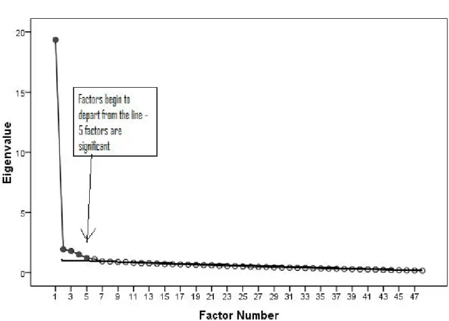
Figure 1. Scree Plot Example
Scree Plot
Unlike other procedures, the scree test provides an easy-to-understand visual approach to determining the number of factors. Catell (1966) noted that significant factors were evident in plots of eigenvalues. Factors that explain random and therefore
similar amounts of variance have very similar eigenvalues that create a straight horizontal line when graphed. Conversely, factors that explain unique systematic variance tend to have larger eigenvalues that rise above the horizontal line created by the random factors, see Figure 1 for an example. All the factors one could draw a line through, going from right to left, are considered inconsequential, and those that are above the line are
considered significant. Cattell (1978) provides an in-depth explanation of this procedure, including solutions to ambiguous graphs.
Standard statistical software that performs factor analysis will print a scree graph. The scree test is more accurate than all the other “easy” alternatives (Cattell &
Vogelmann, 1977; Cliff & Hamburger, 1967; Hakstian, Rogers, & Cattell, 1982). The relatively more labor intensive Parallel Analysis and Minimum Average Partial are the only procedures that have been shown to be more accurate (Velicer, et al., 2000; Zwick & Velicer, 1982, 1986).
The scree test is not without weakness; it tends to overestimate the number of factors. Overestimations occur especially when the sample size is small, there are a large number of factors, or the factor pattern is simple (no significant cross loading or a large number of factors) (Hakstian, Rogers, & Cattell, 1982). However, these situations are the opposite of the special HOFA conditions (low number of variables per factor, low
number of factors), indicating that it may be a good alternative for HOFA.
Unfortunately, the greatest weakness of the scree test is that it is particularly subjective and may lead to a confirmation bias (Crawford & Koopman, 1979); this weakness would also apply to HOFA. Velicer, Eaton, and Fava (2000) have recommended that the scree test only be used as an adjunct to more objective and accurate procedures. Due to the
scree test’s subjectivity, it would be prudent to apply this cautionary advice to HOFA, never-the-less the procedure may maintain some utility in the HOFA situation.
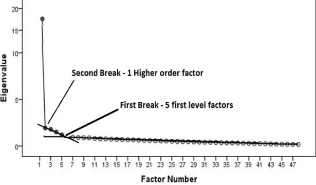
Cattell (1978) has noted that there may be several breaks, or scree, in a single scree plot. Anecdotal evidence suggests this may be caused by differing levels of factors. The first group might be the primary factors and the second group found after the first break might be the secondary factors, and so on and so on. Thus, by examining the various breaks one may be able to identify both the secondary and primary factors by examining one scree plot. Porritt and Boyd (2010) performed a pilot study of these methods, in which the higher multi level methods were able to identify the factor structure in 3 of 4 data sets. In addition to studying traditional scree methods this study will further examine the potential of multi-level scree methods.
Factor Replication (FR)
Everett (1983) proposed that the proper number of factors was the number that best replicated across different samples. He determined this using the coefficient of comparability (Nunnally, 1978), which he notes is comparable to the coefficient of invariance (Pinneau & Newhouse, 1964) for the special case of repeated variables and different subjects. This procedure begins with executing an exploratory factor analysis on random splits of the data set. The factor scores from each half of the data set are than correlated. The correct number of factors is the number for which all factors correlate across subsamples above .9.
McCrae and Costa (1987) successfully used the Everett procedure’s to identify the five factors in their NEO inventory. However, Lanning (1994) experienced
difficulties when using the Everett procedure to identify factors in the California Adult Q test.
Walkey and McCormick (1985b) have also used the logic of replicating factors across subsamples of data. They judged the replicability of factors using Catell’s s index (Cattell, Balcar, Horn, & Nesselroade, 1969) because it provided different estimates for hyperplane cutoffs. They derived the s index using their own FACTOREP computer program (Walkey & McCormick, 1985a) and successfully identified a three factor structure in their data.
As a result of his difficulties with the Q sort Lanning (1996) performed a study comparing MAP and Everett’s Factor Replication. Hefound that MAP and factor replication provided comparable results until the subject to item ratio reached 10:1, at which point factor replication began to grossly over-estimate the number of factors. Based on these findings Lanning asserts that replicability is different from
dimensionality. He concluded that the problematic FR ought to be dropped in favor of MAP. However, one must ask what the point of finding non-replicable dimensionality is. Dimensionality may be statistically significant in a given sample but it fails to have any practical significance if it does not replicate across other samples or subsamples of the same data. A stricter standard like replication may safeguard against dimensionality that is merely an artifact of a given sample, sentiments that have been echoed by Loehlin (2004). Lanning’s primary assertion is that FR should be abandoned for MAP, a measure of dimensionality that is not susceptible to sample size. However, MAP tends to select too few factors when the subject to item ratio is low, as it is in HOFA. On the other hand,
FR is likely to perform well under HOFA conditions because subject to item ratios in HOFA will seldom, if ever, reach 10:1
It is also possible that Everett’s original criterion of correlations above .9 is not strict enough. A given factor can correlate highly with more than one other factor in this case a smaller number of factors would be more appropriate since it combines the highly correlated factors multiple factors into one cohesive factor. To this end, Boyd (reference needed) has recommended a modified criterion of accepting only factors that correlate across subsamples above .9 and have off-diagonal factors that do not come within .08 of the diagonal correlation. It may well be that this improved version of FR is better suited to HOFA conditions than is MAP.
Salient Loadings Criteria (SL)
Wrigley (1960) has proposed that the number of factors be determined by
examining how the variables load on each factor. The proper solution is the one in which every extracted and rotated factor contains at least two variables that load highest on that particular factor. This is derived through a series of factor analysis that begins with an intentional over-extraction and ends when the proper solution is found. Howard & Gordon (1963) have provided an applied example of this procedure. While little
empirical research has been done in regards to this method, it has great potential because it provides a good balance between the judgment of the researcher and a hard
mathematical rule. Gorsuch (1997) has noted this potential and recommended use of this procedure, especially in item analysis.
Hypothesis
Determining the number of factors in HOFA is particularly problematic since the only techniques validated by the empirical research, MAP and PA (Velicer, et al., 2000), are affected by decreases in the ratio of variables to factors (Turner, 1998; Zwick & Velicer, 1986). It is predicted that traditional methods such as PA and MAP will drop below 90% accuracy under HOFA conditions, while non-traditional methods such as scree plots, factor replication and salient loadings will continue to correctly identify the proper number of factors in at least 90% of the datasets.
CHAPTER TWO METHOD
Data
Monte Carlo data often contains clearer factors that do not fully capture the nuances and complexities of respondent-generated data (Zwick & Velicer, 1986). In an attempt to more realistically apply these techniques this study used respondent-generated data from tests with previously verified factor structures. Five established tests with three different sizes of higher-order factor structures were used. Small factor structures,
defined as tests that only have one higher order factor, were represented by the Outcome Questionnaire-45 (OQ-45), and the Wechsler Adult Intelligence Scale – Third Edition (WAIS-III). Medium factor structures, with more than one but less than four higher order factors, were represented by the Child Behavior Checklist/6-18 (CBCL). Large
structures, with four or more higher-order factors, are represented by the International Personality Item Pool NEO (IPIP-NEO), and the 16PF. All analyses were performed on the pre-established primary factor scores created by following the scoring directions in the manual for each test.
Outcome Questionnaire 45
The Outcome Questionnaire 45 (OQ-45)is a 45 item, 5-point Likert, symptom inventory designed to measure outpatient psychotherapy outcomes. The factor structure of three subscales and one general scale has been repeatedly replicated across different cultures (Coco et al., 2008; de Jong et al., 2007). A data set of 4,516 participants
collected from counseling center clients seen by 527 therapists working at 40 university counseling centers throughout the United States was used.
Wechsler Adult Intelligence Scale
The Wechsler Adult Intelligence Scale – Third Edition (WAIS III)is one of the most established and widely used measures of intelligence, with 14 subtests of items administered verbally to individual respondents. Its factor structure and invariance, of four primary factors and one higher order factor, has been well established (Bowden, Weiss, Holdnack, & Lloyd, 2006; Taub, McGrew, & Witta, 2004). A 1,250-subject subsample of the WAIS-III normative sample (The Psychological Corporation, 1997) was obtained.
Child Behavior Check List/ 6-18
The Child Behavior Check List/ 6-18 (CBCL)is a 140 Likert item questionnaire designed to measure psychological symptoms in children. It classifies symptoms into eight narrow-band syndromes and two higher categories, internalizing and externalizing. Three of the primary subscales were dropped from the HOFA because they crossload too strongly on both factors. The results are two higher order factors derived from five primary factors. This factor structure has been replicated with children who have serious emotional disturbances (Dedrick, Greenbaum, Friedman, & Wetherington, 1997), group care workers (Albrecht, Veerman, Damen, & Kroes, 2001) and across 30 different cultures (Ivanova et al., 2007). A sample of 4,994 subjects from the normative sample was purchased.
The International Personality Item Pool NEO
The International Personality Item Pool NEO (IPIP-NEO)is a public measure of personality derived from the International Personality Item Pool, a free to the public pool of items designed to measure personality traits. The IPIP-NEO is meant to measure the same five personality factors as the NEO-PI: Extraversion, Agreeableness,
Conscientiousness, Neuroticism, and Openness to Experience (Goldberg, 1999). Mimicking the NEO-PI, each of the traits is comprised of six facets. Thus there are 30 primary factors and 5 higher order factors. The Higher order factor structure has been replicated across culture (Mlacic & Goldberg, 2007), gender and ethnicity (Ehrhart, Roesch, Ehrhart, & Kilian, 2008), and sexual preference (Zheng et al., 2008). The primary factors have not been empirically verified, but have been theoretically derived to match those of the NEO-PI. A sample of 20,993 internet respondents (Johnson, 2005) was used.
16PF
The16PFis one of the most widely used nonclinical measures of personality. It was one of the first tests to be created using factor analytic procedures, and its sixteen primary and five secondary factor structure has been well established (Aluja, Blanch, & García, 2005; Bonaguidi, Trivella, Michelassi, & Carpeggiani, 1994; Byravan &
Ramanaiah, 1995; Cattell & Cattell, 1995). A data set of parceled items from 4,405 respondents was generously loaned by IPAT Inc. for this study.
Sample Creation
In the interest of creating as many replications as possible while maintaining sufficient power, the larger data sets were divided into smaller data sets by randomly sampling enough participants to establish a ratio of items to participants that was close to 1:10. Since there are only 14 subtests on the WAIS, that data set was split into samples of 200 participants. Saturations for each subsample were obtained by averaging the significant factor loadings across all the factors. Significant factor loadings were defined as items that load above .3 on a given factor and do not have loadings on any other factor that come within .08 of the significant loading. Table 1 shows the average statistics for each group of subsamples.
Table 1
Descriptive statistics for subsamples.
Size I:P ratio Saturation
Mean SD Mean SD Mean SD
# of Samples OQ‐45 452 18.95 1:10 0.00 0.84 0.12 10 WAIS III 208 15.13 1:14 0.00 0.89 0.01 6 CBCL 1,249 20.66 1:11 0.00 0.79 0.01 4 IPIP‐NEO 2,999 42.18 1:09 0.00 0.64 0.03 7 16pf 1,697 28.00 1:08 0.00 0.67 0.00 3 Procedures
Basic descriptions of procedures are provided here; see Appendix A for more detailed instructions regarding implementation of procedures in SPSS. The original
(2000). Fourth-PowerMinimum Average Partial (MAP4) followed the same procedure with O’Conner (2000) syntax altered to raise the trace of the matrix to the fourth-power instead of squaring it.
Parallel analysis and PA95 were performed by obtaining fiftieth percentile and
95th percentile cut-off eigenvalues using O’Connor’s (2000) syntax with 100 random data
sets as recommended by Velicer, Eaton, and Fava (2000). These eigenvalues were than compared to the eigenvalues derived from each dataset. The Kaiser Rule was
implemented using the SPSS roots > 1 option. This procedure is the default in SPSS and automatically extracts all factors with eigenvalues greater than one.
Scree plots were produced from the scree plot option of the Factor Analysis
procedure in SPSS. Tradition scree plots were produced from a factor analysis of the calculated factor scores from each subsample and mulit-level scree plots were produced from the raw data of each subsample. Following the procedures from the pilot study (Porritt & Boyd, 2010), plots of the first 50 eigenvalues were used for scales with more than 50 questions. Both types of scree plots were rated by two independent Judges who had received instruction in a graduate level psychometrics course and read a tutorial by Catell (1978). Inter rater reliability was r=.96 for traditional scree and r=.4 for multi level scree. Disagreements were settled by a third judge.
Factor replication was carried out by randomly splitting the data using the uniform
function in SPSS. Each subsample was then subjected to a series of EFA’s using principal axes extraction with promax (3) rotation and a number of factors decrementing by one, beginning with twice the known number of factors. The factor scores from both
was created. According to Boyd’s rules (Boyd, 2001) replicating factor correlated across the subsamples at .7 or higher, and had no other correlation within.08.
For salient loading criteria the data were exposed to a series of Factor Analysis
using principal axis extraction with Varimax rotation. The series began by extracting twice the known number of factors, and continued with the number of factors being iteratively reduced by one until the analysis yielded a satisfactory structure. Satisfactory structures were defined as a set of factors each of which contained at least two items loading more than .5, or three items loading more than .4 with none of the salient items loading on another factor within .13.
Evaluation Criteria
For the sake of consistency of the literature, the results were evaluated using the same criteria as Velicer, Eaton, and Fava (2000): percent correct, mean difference and standard deviation of the difference. These measures adequately capture overall accuracy, amount of discrepancy, and consistency of each technique.
Percent correct indicates the overall accuracy of a technique. Solutions were considered correct when they identified the known number of factors and incorrect when they failed to do so. The percent correct was determined by dividing the number of correct solutions by the number of the data sets.
Mean difference examines the amount of discrepancy in a technique as defined by how far off the technique estimates on average. The amount of discrepancy for each number of factor solutions is determined by subtracting the known number of factors from the proposed number of factors. Negative values indicate under-extraction, positive
values indicate over-extraction and values of zero indicate a correct answer. The mean difference is the mean of all of these estimates across a set of samples. Technique consistency was measured using the standard deviation of these difference scores.
CHAPTER THREE RESULTS
Most analyses for the study were conducted in SPSS version 17.0. Primary factor scores from the subscales were calculated using the instructions found in the manual for each test. Factor analysis was then performed on these scores, using the various number-of-factor methods.
Percent Correct
Table 2 displays the calculated percent correct for each method. Parallel analysis was the most accurate; each version had overall accuracies of 90% or more. The Kaiser rule, both versions of MAP, and salient loadings criteria were all accurate in 77% of the samples and traditional Scree was slightly less accurate at 63%. Multilevel scree and factor replication were the least accurate with percent correct values at or below 30%.
The OQ-45 and WAIS represented small factor structures as defined by a number primary factors converging into a single general factor. Every method identified these structures with the exception of factor replication and both versions of the scree plot. Traditional Scree was the most accurate of the methods that failed to perfectly identify the structures at this level; identifying the OQ-45’s structure 100% of the time and the WAIS’s structure 83%. Multi-level scree was relatively accurate in the WAIS
subsamples and inaccurate in the OQ-45 subsamples. Factor replication correctly
identified the OQ-45 structure 90% and failed to correctly identify the WAIS-III structure in any of the subsamples.
23
Table 2
Percent correct. Test
# of
Samples MAP MAP4 PA PA95 Kaiser Scree ML Scree FR SL Overall 30 77 77 93 97 77 63 23 30 77 OQ-45 10 100 100 100 100 100 100 20 90 100 WAIS-III 6 100 100 100 100 100 83 83 0 100 CBCL 4 0 0 75 75 100 75 0 0 100 IPIP-NEO 7 100 100 100 100 43 0 0 0 43 16pf 3 0 0 67 100 0 0 0 0 0
The mid-sized factor structures, identified as structures with two to four higher order factors, was represented by the CBCL. The Kaiser Rule and salient loadings criteria successfully identified the proper number of factors for all of the CBCL
subsamples. Traditional scree and both versions of PA only miss-identified the CBCL factor structure in one of the subsamples, for an accuracy of seventy five percent. Multilevel scree, factor replication and both versions of MAP failed to correctly identify the number of factors in any of the subsamples.
The IPIP-NEO and 16pf represented large factor structure defined as structures with five or more higher-order-factors. Both versions of MAP and both versions of PA were able to correctly identify the number of factors in 100% of the IPIP-NEO
subsamples. Both versions of MAP failed to correctly identify the number of factors in any of the 16pf data sets; ninety-fifth percentile PA produced correct solutions for 100% of them and traditional PA only miss-identified one subsample. The Kaiser rule and Salient ladings criteria accurately identified the IPIP-NEO structure in 43% of the subsamples but failed to identify the correct number of factors in any of the 16pf
subsamples. Factor replication and both versions of scree plots failed to properly identify the number of factors in any of the subsamples with large factor structures.
Mean Difference
Table 3 presents the calculated mean differences. Overall traditional PA did not have a mean difference. Ninety-fifth percentile PA and Salient Loadings criteria both slightly under extracted and both versions of MAP moderately under-extracted. The
Kaiser rule moderately over-extracted. Factor replication and both versions of the scree severely over-extracted, each with a mean difference of at least one factor.
With an under extraction for one of the WAIS III subsets, multi-level scree was the only method to under-extract at the small factor structure level (OQ-45 and WAIS III). Factor Replication and multi-level scree were the only two methods to over-extract by an average of one factor at the uncomplicated level. All of the other methods either had a perfect accuracy or slightly over-extracted. Most methods under extracted the mid-sized factor structure of the CBCL subsamples. The only methods that over-extracted for the CBCL subsamples were the traditional scree and Factor replication. Factor Replication and both versions of MAP were the only methods to miss by one or more on average. Every method that was inaccurate for the IPIP-NEO over-extracted. Likewise, every inaccurate method over-extracted for the 16PF with the exception of the salient loadings criteria and both versions of MAP which under-extracted by an average of two factors.
26
Table 3
Mean difference.
MAP MAP4 PA PA95 Kaiser Scree
ML Scree FR SL Overall -0.33 -0.33 0.00 -0.03 0.23 1.47 1.23 1.33 -0.07 OQ-45 0.00 0.00 0.00 0.00 0.00 0.00 1.60 0.10 0.00 WAIS III 0.00 0.00 0.00 0.00 0.00 0.17 -0.17 1.16 0.00 CBCL -1.00 -1.00 -0.25 -0.25 0.00 0.25 -0.50 1.50 0.00 IPIP-NEO 0.00 0.00 0.00 0.00 0.57 4.86 3.29 2.86 0.57 16pf -2.00 -2.00 0.33 0.00 1.00 0.33 0.33 2.00 -2.00
Standard Deviation of the Difference
The calculated standard deviations of the difference scores are in Table 4. Both version of PA had the smallest overall variance in deviations. The Kaiser rule, salient loadings criteria, and both versions of MAP had moderate levels of variation. Multi-level scree and factor replication had overall standard deviation over one, and both versions of the scree plot had the most variance with an overall standard deviation larger than two. When factor structures were small (OQ and WAIS) standard deviations of errors for techniques with less than perfect accuracy were below 0.5 with the exception of multilevel scree, which had a standard deviation of larger than 1.5 within the OQ-45 samples alone. All less than perfect standard deviations for subsamples of mid-sized factor structure (CBCL) were near 0.5 except for multi level scree which had a standard deviation of one. In the subsamples with large factor structures (IPIP-NEO, 16PF) all less than perfect standard deviations for the 16pf were between 0.5 and one with the exception of multi-level scree and factor replication, which had standard deviations over two. Deviations among IPIP-NEO subsamples were much higher. Traditional PA was the only method without perfect accuracy to have a standard deviation under 1. PA95 had offsetting errors and produced a deviation of zero. Despite producing the incorrect solution every time, the Kaiser rule and salient loadings criteria were consistent without any standard deviation in difference scores for the IPIP-NEO subsamples. All other methods had standard deviations of one or greater, both versions of the scree plot had standard deviations over two.
28
Table 4
Standard deviation of difference.
MAP MAP4 PA PA95 Kaiser Scree
ML Scree FR SL Overall 0.71 0.71 0.26 0.18 0.43 2.16 1.94 1.24 0.74 OQ-45 0.00 0.00 0.00 0.00 0.00 0.00 1.51 0.32 0.00 WAIS III 0.00 0.00 0.00 0.00 0.00 0.41 0.41 0.41 0.00 CBCL 0.00 0.00 0.50 -0.50 0.00 0.50 1.00 0.58 0.00 IPIP-NEO 0.00 0.00 0.00 0.00 0.53 0.69 1.70 1.07 0.54 16pf 1.00 1.00 0.58 0.00 0.00 2.08 2.31 1.00 0.00
In order to provide a clearer picture of overall technique consistency and
accuracy, Table 5 provides a breakdown of the percentage of each method’s deviation as a fixed value from the correct number of factors. Both version of PA were accurate and consistent, they were correct over 90% of the time and never missed by more than one factor. The Kaiser Rule and salient loadings criteria were moderately accurate (correct at least 70% of the time) and consistent (never off by more than one factor). Both versions of MAP were moderately accurate (correct at least 70% of the time) and inconsistent (missed by more than one factor at least once). Factor replication and both versions of scree plots were neither accurate nor consistent; they were correct less than 70% of the time and had miss extracted three or more factors at least once.
30
Table 5
Percentage of deviations as a fixed value from the correct solution.
MAP MAP4 PA PA95 Kaiser Scree
ML Scree FR SL +>3 0 0 0 0 0 27 13 7 0 +3 0 0 0 0 0 0 7 13 0 +2 0 0 0 0 0 3 20 17 0 +1 0 0 3 0 23 10 17 33 13 0 77 77 95 97 77 60 23 30 77 -1 17 17 3 3 0 0 20 0 10 -2 3 3 0 0 0 0 0 0 0 -3 3 3 0 0 0 0 0 0 0
CHAPTER FOUR DISCUSSION
The primary hypothesis that traditional techniques will break down under HOFA conditions was partially supported by the data. Both Versions of MAP were accurate in three sets of subsamples, but inaccurate with the smallest item to factor ratios, the CBCL and the 16pf. Likewise, the only errors committed by the two PA methods were in these two sets of subsamples. Of the alternative methods, only two showed promise. The Kaiser rule and salient loading criteria were able to correctly identify the number of factors in all of the CBCL subsamples, something none of the other methods managed to do. However, these methods cannot be viewed as perfect HOFA alternatives. While they were 100% accurate in the three simpler sets of subsets, they lost all accuracy in the tests with a larger number of primary factors. Despite this weakness, they may serve as a useful substitute or concordant methods when both the item to factor ratio and the number of primary factors (or items) are low.
This study was unable to replicate Velicer, Eaton, and Fava’s (2000) findings that MAP4 was more accurate than MAP. Rather the two methods had identical
performances. This may be due to the limited range of the data used in this study. Perhaps, both methods are equally susceptible to limited item to factor ratios. Had a broader range of conditions and data types been used a difference may have emerged. Further examination is needed before any certain conclusions are drawn about MAP4. While this study has exposed a weakness of MAP it has not disproved the technique’s utility. MAP remains the second most accurate and consistent method when working in
data that does not have small item to factor ratio’s, and it use in these situations should in no way be impacted by the results of the current study.
There does appear to be a difference between the two versions of PA. In accordance with theory and research PA95 appears to be more accurate but have a tendency to under extract when it is wrong. However, the current study does not have enough replications to draw any solid conclusions. Prior to making any firm claims further research will need to be conducted with a larger number of replications. PA and PA95 were the only procedures capable of identifying the number of factors in the 16pf sample. Despite weakness when the number of items is low, PA methods remain the most accurate methods over all. Their continued use in all situations is recommended. However, when the number of items is low, it may be useful to supplement the PA findings with those of the Kaiser rule and salient loading criteria.
It is surprising that the Kaiser rule performed so well in these situations. While the limitations of the current data make it impossible to draw causal conclusions with any certainty, one may venture a hypothesis as to its unexpected success. The transition from eigenvalues greater than one to smaller than one was more pronounced in the data with smaller factor structures. As the number of factors increased this transition became more subtle. It is likely that the noise in data with smaller numbers of factors is less present. This favors the simplicity of the Kaiser and simultaneously puts the PA methods at the disadvantage of overcorrecting for error that is not there. This would explain the under extraction of the PA methods when number of factors is low. Further work may reveal a threshold of the number of factors bellow which PA overcorrects and the Kaiser rule is more accurate.
It would seem that the clear jump in eigenvalues has contributed to the accuracy of the scree plot, which remained essentially unchanged under the HOFA conditions. However, this marked decline in HOFA eigenvalues is most likely due to the fact that most HOFA factor structures are non-complex factor structures. Past research (Hakstian, et al., 1982) has established that the scree plot is less accurate when identifying non-complex factor structures. It is likely that this liability counter set the advantages thus resulting in an unchanged accuracy of the scree plot.
Despite promising preliminary research (Porritt & Boyd, 2010) the multi-level scree techniques appears to be problematic. It was the least accurate and least consistent method of all those examined. This could be in large part due to the simpler factor structures in the current data. It could also be that the addition of identifying multiple scree as opposed to one introduces too much ambiguity and subjectivity in a process that is already ambiguous and subjective. Baring further development the use of multilevel scree cannot be recommended at this time.
Next to multi-level scree the factor replication method was the least accurate and least consistent method. This may in large part be due to the large item to factor ratio. Past research has shown that the correlation method of factor replication tends to break down when item to factor ratio approaches 10:1 (Lanning, 1996). Since all of the errors were over factor errors and these errors tend to occur when the number of items is high, it would appear that with high power the correlation method is too sensitive and selects insignificant factors. This may be corrected with some sort of a weight or adjustment to the size of the data. Perhaps correlation is the improper approach to factor replication in large data set. Alternate factor replication criteria may produce better results. It is
important to state that the failure of the current factor replication method does not
disprove the theory of using factor replication to determine the number of factors. It may be a perfectly tenable idea with an improper implementation. Empirical methods for determining factor t invariance are still experimental. It may just be a matter of
developing and perfecting the correct factor replication standard before factor replication techniques can be applied to determining the proper number of factors.
At this point, it is difficult to make a hypothesis as to what is driving the
inaccuracy of the salient loadings criteria. It consistently over factored for the IPIP-NEO and constantly under factored for the 16pf. A larger study with more conditions is needed to ascertain exactly how the salient loadings criteria malfunction in exactly which situations. Until than it appears that the salient loadings criteria is a useful method in cases where there are fewer than 5 higher order factors.
The primary limitations of this study revolve around the use of respondent generated data. Because of this choice, there were a number of variables (i.e. saturation and factor patter complexity) that were not directly controlled. As a result, causal conclusions cannot be made with any degree of certainty. All of the conclusions and observations of this study should be considered tentative until they can be verified in a more closely controlled experiment using Monte Carlo data. What can be said with certainty is that current methods of answering the number of factors question do appear to have certain inconstancies, which have been observed in an applied setting with
REFERENCES
Albrecht, G., Veerman, J. W., Damen, H., & Kroes, G. (2001). The Child Behavior Checklist for group care workers: A study regarding the factor structure. Journal
of Abnormal Child Psychology, 29(1), 83-89.
Allen, S. J., & Hubbard, R. (Writers). (1986). Regression equations for latent roots of random data correlation matrices with unities on the diagonal. [Article],
Multivariate Behavioral Research: Lawrence Erlbaum Associates.
Aluja, A., Blanch, A., & García, L. F. (2005). Reanalyzing the 16pf-5 second order structure: Exploratory versus confirmatory factorial analysis. European Journal of
Psychology of Education, 20(4), 343-353.
Bonaguidi, F., Trivella, M. G., Michelassi, C., & Carpeggiani, C. (1994). The second-order factor structure of Cattell's 16 PF in patients with coronary heart disease.
Psychological Reports, 75(31), 1271-1275.
Bowden, S. C., Weiss, L. G., Holdnack, J. A., & Lloyd, D. (2006). Age-related
invariance of abilities measured with the Wechsler Adult Intelligence Scale-III.
Psychological Assessment, 18(3), 334-339.
Boyd, K. C. (2001). Factor replication as a criterion for number of factors in exploratory
factor analysis of items. 61, ProQuest Information & Learning, US. Retrieved
from http://0-search.ebscohost.com.catalog.llu.edu/login.aspx?direct=true&db =psyh&AN=2001-95006-334&site=ehost-live
Buja, A., & Eyuboglu, N. (1992). Remarks on parallel analysis. Multivariate Behavioral
Research, 27(4), 509-540.
Byravan, A., & Ramanaiah, N. V. (1995). Structure of the 16 PF fifth edition from the perspective of the five-factor model. Psychological Reports, 76(2), 555-560. Cattell, R. B. (1966). Scree test for number of factors. Multivariate Behavioral Research,
1(2), 245-276.
Cattell, R. B. (1978). The scientific use of factor analysis in behavioral and life sciences New Yourk, NY US: Plenum Press.
Cattell, R. B., Balcar, K. R., Horn, J. L., & Nesselroade, J. R. (1969). Factor matching procedures: An improvement of the S index; with tables. Educational and
Psychological Measurement, 29(4), 781-792.
Cattell, R. B., & Cattell, H. E. P. (1995). Personality structure and the new fifth edition of the 16PF. Educational and Psychological Measurement, 55(6), 926-937. doi: 10.1177/0013164495055006002
Cattell, R. B., & Vogelmann, S. (1977). A comprehensive trial of the scree and KG criteria for determining the number of factors. Multivariate Behavioral Research, 12(3), 289-325.
Cliff, N., & Hamburger, C. D. (1967). The study of sampling errors in facto analysis by means of artificial experiments. Psychological Bulletin, 68(6), 430-445.
Coco, G. L., Chiappelli, M., Bensi, L., Gullo, S., Prestano, C., & Lambert, M. J. (2008). The factorial structure of the Outcome Questionnaire-45: A study with an Italian sample. Clinical Psychology & Psychotherapy, 15(6), 418-423.
Cota, A. A., Longman, R. S., Holden, R. R., & Fekken, G. C. (1993). Interpolating 95th percentile eigenvalues from random data: An empirical example. Educational and
Psychological Measurement, 53(3), 585-596.
Crawford, C. B., & Koopman, P. (1979). Note: Inter-rater reliability of scree test and mean square ratio test of number of factors. Perceptual and Motor Skills, 49(1), 223-226.
de Jong, K., Nugter, M. A., Polak, M. G., Wagenborg, J. E. A., Spinhoven, P., & Heiser, W. J. (2007). The Outcome Questionnaire (OQ-45) in a Dutch population: A cross-cultural validation. Clinical Psychology & Psychotherapy, 14(4), 288-301. Dedrick, R. F., Greenbaum, P. E., Friedman, R. M., & Wetherington, C. M. (1997).
Testing the structure of the Child Behavior Checklist/4-18 using confirmatory factor analysis. Educational and Psychological Measurement, 57(2), 306-313. Derogatis, L. R., Serio, J. C., & Cleary, P. A. (1972). An empirical comparison of three
indices of factorial similarity. Psychological Reports, 30(3), 791-804.
Ehrhart, K. H., Roesch, S. C., Ehrhart, M. G., & Kilian, B. (2008). A test of the factor structure equivalence of the 50-item IPIP Five-factor model measure across gender and ethnic groups. Journal of Personality Assessment, 90(5), 507-516. Everett, J. E. (1983). Factor comparability as a means of determining the number of
factors and their rotation. Multivariate Behavioral Research, 18(2), 197-218. Everett, J. E., & Entrekin, L. V. (1980). Factor comparability and the advantages of
multiple group factor analysis. Multivariate Behavioral Research, 15(2), 165-180. Fabrigar, L. R., Wegener, D. T., MacCallum, R. C., & Strahan, E. J. (1999). Evaluating
the use of exploratory factor analysis in psychological research. Psychological
Methods, 4(3), 272-299.
Fava, J. L., & Velicer, W. F. (1992). The effects of overextraction on factor and component analysis. Multivariate Behavioral Research, 27(3), 387-415.
Fava, J. L., & Velicer, W. F. (1996). The effects of underextraction in factor and component analyses. Educational and Psychological Measurement, 56(6), 907-929.
Glorfeld, L. W. (1995). An improvement on Horn's parallel analysis methodology for selecting the correct number of factors to retain. Educational and Psychological
Measurement, 55(3), 377-393.
Goldberg, L. R. (1999). A broad-bandwidth, public domain, personality inventory measuring the lower-level facets of several five-factor models. Personality
psychology in Europe, Vol. 7. (Vol. 7, pp. 7-28). Tilburg Netherlands: Tilburg
University Press.
Gorsuch, R. L. (1980). Factor score reliabilities and domain validities. Educational and
Psychological Measurement, 40(4), 895-897.
Gorsuch, R. L. (1983). Factor Analysis (2nd Ed.). Hillsdale, NJ US: Lawrence Erlbaum Associates, Inc., Publishers.
Gorsuch, R. L. (1997). Exploratory factor analysis: Its role in item analysis. Journal of
Personality Assessment, 68(3), 532-560.
Guttman, L. (1954). Some necessary conditions for common-factor analysis.
Psychometrika, 19, 149-161.
Hakstian, A. R., Rogers, W. T., & Cattell, R. B. (1982). The behavior of number-of-factors rules with simulated data. Multivariate Behavioral Research, 17(2), 193-219.
Hayton, J. C., Allen, D. G., & Scarpello, V. (2004). Factor Retention Decisions in Exploratory Factor Analysis: A Tutorial on Parallel Analysis. Organizational
Research Methods, 7(2), 191-205.
Horn, J. L. (1965). A rationale and test for the number of factors in factor analysis.
Psychometrika, 30(2), 179-185.
Howard, K. I., & Gordon, R. A. (1963). Empirical note on the 'number of factors' problem in factor analysis. Psychological Reports, 12(1), 247-250.
Humphreys, L. G., & Montanelli, R. G. (1975). An investigation of the parallel analysis criterion for determining the number of common factors. Multivariate Behavioral
Research, 10(2), 193-205.
Ivanova, M. Y., Achenbach, T. M., Dumenci, L., Rescorla, L. A., Almqvist, F.,
Weintraub, S., . . . Verhulst, F. C. (2007). Testing the 8-syndrome structure of the Child Behavior Checklist in 30 societies. Journal of Clinical Child and
Johnson, J. A. (2005). Ascertaining the validity of individual protocols from Web-based personality inventories. Journal of Research in Personality, 39(1), 103-129. doi: 10.1016/j.jrp.2004.09.009
Kaiser, H. F. (1960). The application of electronic computers to factor analysis.
Educational and Psychological Measurement, 20, 141-151.
Lanning, K. (1994). Dimensionality of observer ratings on the California Adult Q-set.
Journal of Personality and Social Psychology, 67(1), 151-160.
Lanning, K. (1996). Robustness is not dimensionality: On the sensitivity of component comparability coefficients to sample size. Multivariate Behavioral Research, 31(1), 33-46.
Lautenschlager, G. J. (1989). A comparison of alternatives to conducting Monte Carlo analyses for determining parallel analysis criteria. Multivariate Behavioral
Research, 24(3), 365-395.
Lautenschlager, G. J., Lance, C. E., & Flaherty, V. L. (1989). Parallel analysis criteria: Revised equations for estimating the latent roots of random data correlation matrices. Educational and Psychological Measurement, 49(2), 339-345. Lee, H. B., & Comrey, A. L. (1979). Distortions in a commonly used factor analytic
procedure. Multivariate Behavioral Research, 14(3), 301-321.
Longman, R. S., Cota, A. A., Holden, R. R., & Fekken, G. C. (1989). A regression
equation for the parallel analysis criterion in principal components analysis: Mean and 95th percentile eigenvalues. Multivariate Behavioral Research, 24(1), 59-69. McCrae, R. R., & Costa, P. T. (1987). Validation of the five-factor model of personality
across instruments and observers. Journal of Personality and Social Psychology, 52(1), 81-90.
Mlacic, B., & Goldberg, L. R. (2007). An analysis of a cross-cultural personality inventory: The IPIP Big Five factor markers in Croatia. Journal of Personality
Assessment, 88(2), 168-177.
Nunnally, J. C. (1978). Psychometric theory (2nd Edition). New York, NY US: McGraw-Hill.
O'Connor, B. P. (2000). SPSS and SAS programs for determining the number of components using parallel analysis and Velicer's MAP test. Behavior Research
Methods Instruments & Computers, 32(3), 396-402.
Pinneau, S. R., & Newhouse, A. (1964). Measures of invariance and comparability in factor analysis for fixed variables. Psychometrika, 29(3), 271-281.
Taub, G. E., McGrew, K. S., & Witta, E. L. (2004). A Confirmatory Analysis of the Factor Structure and Cross-Age Invariance of the Wechsler Adult Intelligence Scale-Third Edition. Psychological Assessment, 16(1), 85-89.
Thurstone, L. L. (1947). Multiple-factor analysis; a development and expansion of The
Vectors of Mind. Chicago, IL US: University of Chicago Press.
Turner, N. E. (1998). The effect of common variance and structure pattern on random data eigenvalues: Implications for the accuracy of parallel analysis. Educational
and Psychological Measurement, 58(4), 541-568.
Velicer, W. F. (1976). Determining the number of components from the matrix of partial correlations. Psychometrika, 41(3), 321-327.
Velicer, W. F., Eaton, C. A., & Fava, J. L. (2000). Construct explication through factor or component analysis: A review and evaluation of alternative procedures for
determining the number of factors or components. In R. D. Goffin & E. Helmes (Eds.), Problems and solutions in human assessment: Honoring Douglas N.
Jackson at seventy. (pp. 41-71). New York, NY US: Kluwer Academic/Plenum
Publishers.
Walkey, F. H., & McCormick, I. A. (1985a). FACTOREP: A Pascal program to examine factor replication. Educational and Psychological Measurement, 45(1), 147-150. Walkey, F. H., & McCormick, I. A. (1985b). Multiple replication of factor structure: A
logical solution for a number of factors problem. Multivariate Behavioral
Research, 20(1), 57-67.
Wood, J. M., Tataryn, D. J., & Gorsuch, R. L. (1996). Effects of under- and overextraction on principal axis factor analysis with varimax rotation.
Psychological Methods, 1(4), 354-365.
Wrigley, C. (1960). A procedure for objective factor analysis. Paper presented at the
Society of Multivariate Experimental Psychology., 41(3), 321-327.
Zheng, L., Goldberg, L. R., Zheng, Y., Zhao, Y., Tang, Y., & Liu, L. (2008). Reliability and concurrent validation of the IPIP Big-Five factor markers in China:
Consistencies in factor structure between internet-obtained heterosexual and homosexual samples. Personality and Individual Differences, 45(7), 649-654. Zwick, W. R., & Velicer, W. F. (1982). Factors influencing four rules for determining the
number of components to retain. Multivariate Behavioral Research, 17(2), 253-269.
Zwick, W. R., & Velicer, W. F. (1986). Comparison of five rules for determining the number of components to retain. Psychological Bulletin, 99(3), 432-442.
APPENDIX A
DETAILED DESCRIPTION OF METHODS
Kaiser Rule
The Kaiser rule was implemented using the roots greater than option in SPSS. From the primary factor analysis window select extraction options. This will open the “Extraction Options” window as seen in Figure 2. Locate the roots greater than dialog box and enter a one, this will extract all factors with an eigenvalue grater than 1. It should be noted that this is the default option in SPSS.
Figure 3. Mulit-Level Scree Plot Example.
Scree Plot
SPSS will automatically produce scree plots for any factor analysis. Simply check the scree plot box in the extraction options window and a scree plot will be shown in the output window along with the other results from the analysis. A straight edge is then used to determine which points create a line and which points jump over the line. The initial point that departs from this line is the first one counted. Every other point after that is than counted as a significant factor, see Figure 3. In Multi-Level Scree one follows the same procedures for obtaining the scree plot and finding the first scree. The second scree is determined by using the first counted dot, which is the first dot that departs from the first scree, as the first dot in the new scree. Starting from this dot all subsequent dots that can be connected by a straight line form the new scree. Each scree must consist of at least
three dots. This procedure is continued until the researcher can no longer find scree consisting of at least three dots that do not belong to any of the previous scree.
Minimum Average Partial: Traditional and 4th Power
Despite its accuracy, Minimum Average Partial (MAP) is not currently available as an option in SPSS. However, O'Connor (2000) has provided syntax that will reliably and proficiently perform the MAP procedure (Figure 4). This syntax provides a print out of the average squared partial correlations for each iteration, identifies the lowest
average, and prints out the proper number of factors. Prior to running the syntax the researcher needs to change the underlined text on lines 1 and 2 to specify the proper list of variables for the analysis. Variables can be listed one by one, however, if the variables are located sequentially in the file without a break the researcher can use the name of the first variable the “to” command and the name of the last variable as is shown in this example. The researcher will also need to change the italicized text on lines 1 and 2 to specify a file location on their computer. This file name will correspond to a working file the program creates as it runs. The working file is used solely for internal processes of the syntax; the researcher will never need to look at the contents of these files and may choose to delete them after analysis. After making the appropriate changes to the syntax the researcher can than run the syntax, which will than print the results to the most recently used output window.
A sample of the O’Connor results print out can be seen in figure 5. The printed results begin with the eigenvaules of every possible factor, located under the heading “eigenvalues”. After the eigenvalues the researcher will find two columns under the