Variable Selection and Inference in a follow-up Study on Back Pain

Wippert

Variable Selection and Inference in a follow-up

Study on Back Pain

Technical Report Number 211, 2017 Department of Statistics

University of Munich

follow-up Study on Back Pain

David Drießlein

, Helmut K¨

uchenhoff

, Gerhard

Tutz

and Pia-Maria Wippert

1 _{Department of Statistics, Ludwig-Maximilians-Universit¨at (LMU), Munich,}

Ger-many

2 _{Department of Sociology of Physical Activity and Health, University Potsdam,}

Ger-many

Address for correspondence: Helmut K¨uchenhoff, Statistisches Beratungslabor StaBLab, Institut f¨ur Statistik, Ludwig-Maximilians-Universit¨at M¨unchen, Akademiestr.1 80799 M¨unchen, Germany.

E-mail: [email protected].

Phone: +49 89 2180 2789.

Fax: +49 89 2180 5308.

Abstract: The Lasso of Tibshirani (1996) is a useful method for estimation and implicit selection of predictors in a linear regression model, by using a `1-penalty, if

the number of observations is not markedly larger than the number of possible pre-dictors. We apply the Lasso to a predictive linear regression model in a study with baseline and follow up measurement for unspecific low back pain with a focus on the

selection of psycho sociological predictors. Practitioners want to report measures of uncertainty for estimated regression coefficients, i.e. p-values or confidence intervals, where post selection classical t-tests are not valid anymore. In the last few years several approaches for inference in high-dimensional data settings have been devel-oped. We do a selective overview on assigning p-values to Lasso selected variables and analyse two methods in a simulation study using the structure of our data set. We find out that Multi Sample Splitting (Wasserman and Roeder, 2009; Meinshausen et al., 2009) may not be helpful for generating p-values, while the LDPE approach of Zhang and Zhang (2014) produces promising results for type-I-errors and power calculations on single hypotheses. Therefore, we apply the LDPE for the analysis of our back pain study.

Key words: Lasso; Multi Sample Splitting; LDPE; inference; post selection infer-ence, MiSpEx Network

1

Introduction

1.1

Variable Selection via the Lasso

The analysis of high-dimensional data occurs in a multitude of scientific disciplines. Therefore, the development and improvement of appropriate statistical methods plays an important role for regression models being applicable in high dimensional predic-tors to achieve a selection of relevant predicpredic-tors. A selective review for variable selection in high-dimensional situations is given by Fan and Lv (2010).

The Lasso ofTibshirani(1996), a regularization approach based on the`1-norm of the

coefficient vector enables an estimation of the unknown parameter vector in a linear regression model, as well as an implicit variable selection. With its straightforward applicability, its interpretability equivalent to regression models and a multitude of established implementations in R the Lasso commends itself to practitioners. In contrast to the common approach of stepwise selection the Lasso allows a continuous and simultaneous selection while penalizing the coefficients in the regression model. In the current literature, a strong theoretical foundation of Lasso properties has been given, as well as different efficient and fast algorithms. Additionally the Lasso has been extended to further model classes than linear regression models, see e.g. Groll and Tutz(2014). On the other hand, there is limited opportunity to achieve inferential guarantees for a Lasso selected model or its (refitted) coefficients. Statistical inference for Lasso is a contemporary open field of research, which has gathered increasing attention in the past few years. The steady growing literature and research proposes different approaches and methods to do inference in high-dimensional data settings and especially for the Lasso.

1.2

Outline

In the following section, we describe our data set and specify the goal of a predictive model for back pain, with 174 possible predictors. Section3characterizes the problem of statistical inference after a selection procedure and gives an overview about different inference approaches associated with a Lasso selection. The Multi Sample Splitting (MSS) approach of Wasserman and Roeder(2009) andMeinshausen et al.(2009) and the Low Dimensional Projection Estimator (LDPE) of Zhang and Zhang (2014) are

emphasized, on which we base our simulation study of section 4. The application of Lasso selection to our data set, as well as possible inference results are presented in section 5. Conclusively we summarize and discuss our results in section6.

2

Data and aims

2.1

Epidemiological background

Low back pain (LBP) is a musculoskeletal problem which can lead to long-term disability and frequent use of health services (Ibrahim et al., 2008). The lifetime prevalence of LBP is around 84% (Airaksinen et al., 2006). Germany shows a rate of 80% with a point prevalence of 30–40% and yearly costs between 16–22 billion Euro (Gesundheitsreport ,2014). Many LBP episodes only last for a few days/weeks and resolve spontaneously, but around 40% of patients develop persistent problems (Menezes Costa et al., 2012). For this group LBP is a socioeconomic burden leading to an economic problem for health services and an increase in long-term disability claims. The yearly treatment costs for LBP patients at rehabilitation clinics are around 2 billion Euro (Statistisches Bundesamt, 2010). These costs can be reduced if high-risk patients are identified at an early stage. Prognostic factors for LBP chronicity include psychosocial factors such as stress, anxiety, depression or social isolation (Nicholas et al., 2011). Several research groups have developed standards for the identification of prognostic factors and the conduction of prognosis studies for LBP (e.g. PROGRESS,Hemingway et al.(2013),Riley et al.(2013),Hingorani et al.

with an easy screening which warns of potential poor outcomes. Existing screening tools [Hill et al. (2008),Hill et al.(2010),Traeger et al. (2015),Traeger et al. (2016),

Lentz et al. (2016)], are mainly used for secondary prevention and based on experts opinion. Further they suffer from a short prognosis time frame (only Janwantanakul et al.(2015) offer a one-year prognosis) and from a statistical point of view from weak mathematical or algorithmic models. The objective of our analysis is the identification of psycho-sociological indicators for a one-year predictive model for chronic unspecific back pain.

2.2

Data

Design: The data originate from a longitudinal study in whichn = 1071 participants were consecutively enrolled at four clinical study sites in Germany. Finally n = 1046 participants (age: M = 40.4 ys., SD = 13.4, f = 57%, m = 43%) were assessed at the beginning and six further measurement points (M1 to M7) over a two-year period (date range 02/2012 until 08/2014). The study methodology was previously described in detail by Wippert et al. (subm.).

Participants: Participants were eligible for study if they were between 18 and 65 years old, able to speak and read German, suffering from nonspecific low back pain and contacting the doctor for the first time about LBP. Exclusion criteria were suffering from acute pain (last 7 days), inability to stand upright, complete a questionnaire, give sick leave information or showing red flags (e.g. inflammatory diseases). All patients provided written informed consent prior to study participation and received written and oral information about the project.

baseline from M1 and was assessed by the Chronic Pain Grade questionnaire (CPG;

Von Korff et al. (1992)) using the scale for subjective pain intensity (PI:0 = no pain to100 = the worst pain imaginable) in the past three months. The total score from 0 to 100 based on additively aggregated items inquiring subjective pain strength of par-ticipants. Psychosocial risk factors and potential predictors were gained by different standardized questionnaire which are usually used for the assessment of yellow flags. At baseline, sociodemographic factors (e.g. sex, age, job, education, income (Lechert et al., 2006)), medical care (Pfingsten et al., 2007) and lifestyle factors (individual sleep and health satisfaction, weekly duration of sporting activity, smoking and alco-hol behaviour, use of medicines) were assessed as well as all dynamic characteristics (personality states) including Fear-Avoidance, Chronic Stress, Anxiety and Depres-sion, Vital Exhaustion, Sleep and Health Behavior, relationships. In detail: Fear-Avoidance were gathered by the Fear-Fear-Avoidance-Beliefs-Questionnaire (FABQ-D, Pf-ingsten et al. (1997)), chronic stress by the Trier Inventory for chronic stress (TICS,

Schulz et al. (2004)), Anxiety and depression by the German Hospital Anxiety and Depression Scale (HADS-D, Herrmann et al. (1995)), vital exhaustion by the Maas-tricht Vital Exhaustion Questionnaire (VE, MaasMaas-tricht Vital Exhaustion, Schnorpfeil et al. (2002)) and relationships by the attachment category model (Bartholomew and Horowitz,1991). Further self-efficacy (I-SEE, Inventory for the Measurement of Self-Efficacy and Externality, Krampen (1991)), Social Support (Berlin Social Support Scales, Schwarzer and Schulz (2000)) and Life events were assessed as well as fear avoidance and endurance behavior was gathered by the Pain Persistence Scale of the Avoidance-Endurance-questionnaire (AEQ-PPS, Hasenbring et al.(2009)).

3

Inference approaches for Lasso

The core task of statistical inference in the sense of hypothesis testing and confidence intervals is to quantify uncertainty of estimators. Compared to the state of research for methods, algorithms and properties of the Lasso, statistical inference is developed far less. For a practitioner, who wants to use the Lasso to get a selection of the most influential predictors, it might be useful to access p-values and confidence intervals for the estimated coefficients of selected predictors. The simple Lasso-estimator is infeasible for hypothesis testing. On the one hand it is not representable in a closed form and therefore has no explicit distribution, on the other hand, it is not possible to determine a limiting distribution. Its distribution is non steady with point mass in zero (Knight and Fu, 2000) making classical bootstrap invalid. Furthermore refitting the selected predictors in a regression model and placing inference on the usual t-statistic is invalid after a previous variable selection.

A variety of approaches has been proposed using the sample once or multiply, assess-ing the hypothesis testassess-ing unconditioned or conditioned on the selection procedure. We consider two approaches in our simulation study: The Multi Sample Splitting (MSS) of Wasserman and Roeder (2009) andMeinshausen et al.(2009) and the Low dimensional projection estimator (LDPE) of Zhang and Zhang (2014), which are explained in detail in the following subsections.

3.1

Multi Sample Splitting (MSS)

The fundamental approach of applying sample splitting for generating p-values is given by Wasserman and Roeder (2009). In a simple version the data set is split

into two parts. On the first part a Lasso selection is done by cross validating the optimal penalty strength. Thereafter the coefficients of selected variables are refitted in a linear regression model on the second part of the data set. The usual t-statistic, which serves for calculation of p-values stays valid, if independent sample splits are used for selection and inference. Meinshausen et al. (2009) extend this approach to a repetition of splitting, selection and calculation of p-values and a final aggregation of multiple p-values for each predictor, while controlling the family wise error rate (FWER). The repeated splitting is less sensitive regarding the selection of a single split.

A formal description illustrates the steps in detail: For sample splitting repetition

b = 1, . . . , B the data is randomly split into two disjunct subsets with row indices

I₁(b), I₂(b) ⊂ {1, . . . , n} for which |I₁(b)| = bn/2c, |I₂(b)| = n − bn/2c, I₁(b) ∩ I₂(b) = ∅ and therefore I₁(b) ∪ I₂(b) = {1, . . . , n}. Applying the Lasso on the subset with indices I₁(b) returns the indices ˆS(b) _{⊂ {1, . . . , p} for selected predictors, for which}

is assumed |Sˆ(b)_{| ≤ |I}(b)

1 | = bn/2c ≤ |I (b)

2 | in order to achieve subsequently a least

squares estimation on the second half of the data set with indices I₂(b). While the corresponding p-values ˜P_j(b), j ∈Sˆ(b) _{are based on the model, the p-values of all other}

variables are assumed to take a value of one: ˜P_j(b)= 1, j /∈Sˆ(b)_.

In order to aggregate the for multiple testing adjusted p-values P_corr,j(b) = min( ˜P_j(b)_·

|Sˆ(b)_{|,1), j = 1, . . . , p, b = 1, . . . , B over B repetitions, quantiles of their empirical}

distributions are calculated. With γ _∈(0,1) and the empirical quantile function qγ(·)

Qj(γ) = min n

qγ(Pcorr,j(b) /γ;b= 1, . . . , B),1 o

, j = 1, . . . , p (3.1) gives for every fixed value of γ multiple testing adjusted p-values for each covariate. Finding an optimal value for γ, whilst ensuring a FWER-control is proposed to be

data driven and achieved through

Pj = min

(1₋logγmin)· inf γ∈(γmin,1)

Qj(γ),1

, j = 1, . . . , p (3.2) with γmin ∈ (0,1) and recommended by Meinshausen et al. (2009) to be 0.05. The

adaptive search for an optimal value ofγis compensated through the correction factor (1−logγmin).

Compared to a single sample split, the repetition of selection and inference allows some stability and reproducability regarding the aggregated p-values. The approach centers on the control of FWER, aiming the asymptotic validity of P(V > 0) _≤ α, with V denoting the number of falsely rejected null hypotheses. This is succeeded by the adjusted, aggregated p-values of equation (3.2) and a p-value based variable selection.

Meinshausen et al. (2009) point out the suitability of MSS compared to least squares (LS) estimation, if the ratio n/p < 1.5. An intuitive explanation is the increasing variance of LS-estimates, which reduces the ability to determine relevant coefficients. In our simulation study, we consider unadjusted calculated p-values in equation (3.1).

3.2

Low dimensional projection estimator (LDPE)

Zhang and Zhang (2014) propose a method, bias correcting a linear estimator for regression coefficients and constructing confidence intervals based on an asymptotic distribution for the estimator.

To understand their approach it is useful to draw on the geometrical interpretation of the LS-estimator. The outcome vector y_∈Rn _{is projected into the column space of}

X _∈Rn×p_{, which is put up by the linear independent covariate vectorsx}(1)_{, . . . ,x}(p) _∈

Rn_{. The predicted vector ˆy is the projection into the column space and is orthogonal}

to the residual vector ˆ, such that ˆ0yˆ = 0. In addition ˆ is located in the orthogonal complement of the column space, i.e. ˆ0x(j)_{= 0, ∀j = 1, . . . , p.}

An alternative formulation for the LS-estimator is given by ˆβj;LS = y

0(j)

x(j)0(j) with

(j) _{denoting the residual vector of regressing x}(j) _{on the design matrix without the}

column of the j-th covariate X(−j). For all k 6= j: (j)0_x(k) _{= 0. In the case p > n}

a regularized projection of x(j) _{on X}(−j) _{is necessary, therefore the residuals z}(j)

are calculated by a cross validated Lasso model. Cause there exists no z(j) _being

orthogonal to the p−1 column vectors,x(k)0_z(j) _{= 0 is not fulfilled for j 6=k.}

Equivalent to the LS-estimator a linear estimator is given by ˆ βj = y0_z(j) x(j)0_z(j) =βj∗+ 0_z(j) x(j)0_z(j) + X k6=j x(k)0 z(j) x(j)0_z(j)βk∗ (3.3)

where y has been replaced by the model equation. While in the case of p < n with

x(k)0_z(j) _{= 0 the sum over k 6= j is removed, for p > n every covariate contributes}

linearly to an unavoidable bias of ˆβj, caused by x(k)

0

z(j)_{6= 0. The authors propose a}

correction of this bias by adducting the Lasso estimators ˆβk,lasso ofy regressed onX

as initiating estimator for β_k∗ (k6=j), such that ˆ bj = ˆβj − X k6=j x(k)0 z(j) x(j)0_z(j)βˆk,lasso = y0_z(j) x(j)0_z(j) − X k6=j x(k)0 z(j) x(j)0_z(j)βˆk,lasso (3.4)

gives a bias corrected estimator. Zhang and Zhang (2014) call this estimator low dimensional projection estimator (LDPE) and show that under suitable conditions

√ n(ˆbj −βj∗) σΩ1jj/2 a ∼N(0,1) with Ωjj = z(j)0 z(j) (z(j)0_x(j))2 ∀j = 1, . . . , p. (3.5)

Using an estimate ˆσ2

for the residual variance hypotheses can be tested and

(si-multaneous) confidence intervals constructed. The possibility of an implicit variable selection may be given by selecting covariates, whose estimated coefficients exceed a predefined threshold. Lockhart et al.(2014b) state that it is not clear how to connect p-values calculated by this approach to Lasso selected variables, in a sense of post selection inference.

3.3

Further approaches

Beside the two approaches we investigate in our simulation study, there are further ideas and developments for high-dimensional inference. A variety of approaches has been proposed using the sample once or multiply, assessing the hypothesis testing unconditioned or conditioned on the selection procedure. These include a modified bootstrap procedure, see Chatterjee and Lahiri (2011). Javanmard and Montanari

(2014) propose an estimator given by the simple formula ˆθcorr = ˆθlasso+1_nM X0(y−

Xθˆlasso) correcting the bias of the Lasso estimator ˆθlasso. The key role is played by

the matrix M, serving to de-correlate the columns of the design X. Under given assumptions the distribution of ˆθcorr is approximately Gaussian, which allows the construction of confidence intervals and p-values.

The covariance test statistic of Lockhart et al.(2014a) is a novel approach within the Lasso framework, proposing a conditional test sequence oriented by the coefficient paths of a Lasso selection. The coefficient paths of a Lasso estimation represent the order in which predictors with non-zero coefficients at decreasing degree of penaliza-tion are chosen for the Lasso model. Their test sequence is based on the null hypothe-sis that a Lasso model at a given penalty degree contains all truly active variables and

therefore tests the significance of a predictor entering this model. B¨uhlmann et al.

(2014) point out, that compared to fixed tests on single predictors, the conditional hypothesis do not allow an interpretation of p-values in the classical sense.

3.4

Implementation in R

With implementations for different inference approaches the R-package hdiof Meier et al. (2014) allows the construction of p-values and confidence interval in high-dimensional settings. Dezeure et al. (2015) compare those implemented approaches regarding power calculations and familywise error rates in a wide range of simulation studies.

4

Simulation study

To evaluate the reliability and performance of the two chosen inference approaches MSS and LDPE in our concrete data problem, we ran a simulation study. We create the setting similar to our data set. This should allow us to assess the performance of both methods regarding practical applicability and their sensitivity in the underlying data. As computational implementation of these methods inRserves the packagehdi

from Meier et al. (2014) and the therein contained functions multi.split for MSS and lasso.proj for LDPE.

4.1

Setup and evaluation criteria

We chose a simulation setting with n = 200 observations and 174 predictors, which corresponds to the application we consider. To obtain a data structure that is close to the application the observed predictors in the simulation were sampled randomly from the real data set. The data set on which our simulation was built contained 171 predictors, the baseline-measurement of pain intensity and the control variables sex and age. Since the Lasso selects 15 predictors we chose p∗ _{= q+ 3 = 15 active}

predictors. A two step procedure describes the assignment of active predictors and their assumed true coefficient values:

1. The lasso.firstq-function from hdi determines the first q variables selected on the Lasso-path from a Lasso-model that includes 171 items, sex, age and the baseline as predictors and the intensity of pain as outcome.

2. A linear model (LM) with the selected q variables and the fixed variables sex, age and the baseline (y1) is used to estimate the coefficients βy∗1, β

∗

. . ., β∗

q, which were interpreted as the true variable weights. In addition one

obtains an intercept β∗

0 and the residual varianceσLM2 .

New outcome values ysim

i for individualiwere generated by using the linear predictor

consisting of the q selected variables and three fixed variables:

ysim_i =β₀∗+yi,1·βy∗1 +xi,sex·β

∗

sex+xi,age·βage∗ +xi,1·β1∗+. . .+xi,q·βq∗+, (4.1)

where _∼ N(0, c2 _·σˆ2

LM) denotes a randomly chosen error term, which uses the

residual variance of the linear model and a factor c_{∈ {}1₃,2₃,1_}, which allows to vary the dispersion of the simulated outcomes.

The main simulation scenario containsB = 30 repetitions, where the above mentioned model serves as a base model. For each repetitionb = 1, . . . , B the design matrix Xb

varies by the repetition specific n = 200 observations (rows), randomly sampled from the complete data set of 395 observations. Additionally in each of the B repetitions with design Xb, 100 different versions of the outcome values for each observation in

Xb were simulated according to the linear model. These 100 outcome versions, which

are called inner repetitions, allow to compute 100 estimated p-values for each of the predictors in every repetition b= 1, . . . , B.

The p-values are based on the predictor specific hypothesisH0,j :βj∗ = 0 vs. HA,j :

β∗

j 6= 0, j = 1, . . . , p. The p-values of the inactive predictors j ∈ S∗ = {j : βj∗ =

0, j = 1, . . . , p_} were used to determine the type-I-error, the p-values of the active predictors j _∈ S∗ _{= {j : β}∗

j 6= 0, j = 1, . . . , p} were used to determine the power,

1) To obtain an empirical version of thepowerfor a single hypothesis as the proba-bility of rejecting the null hypothesis,P(H0,j is rejected, j∈S∗), we used the number

of cases of the inner repetitions, in which a p-value beneath the fixed significance level

α = 0.05 was generated. The corresponding empirical power was computed by

Powerj = 1 B B X b=1 1 L L X `=1 I(p`,b_j ≤0.05) ! , j ∈S∗, (4.2)

where ` = 1, . . . , L (L= 100) denotes the inner repetitions, in which for fixed design an outcome vector y` _{was simulated that yielded the p-value for variable j p}`,b

j . I(.)

denotes the indicator function, taking the value 1, if p`,b_j ≤0.05, and 0 otherwise.

2) For inactive predictors the type-I-error is reported, giving the probability of falsely rejecting the null hypothesis,P(H0,j is rejected, j ∈S∗). The empirical version

was computed by type-I-error_j = 1 B B X b=1 1 L L X `=1 I(p`,b_{j ≤}0.05) ! , j _∈S∗_{. (4.3)}

4.2

Results

The p-values generated by MSS and LDPE are first used to compute the power and the type-I-error for each predictor and each repetition aggregated over the inner repetitions. Then we consider the aggregation over all repetitions. We distinguish varying degrees of dispersion and compare the presented results to scenarios that are not shown.

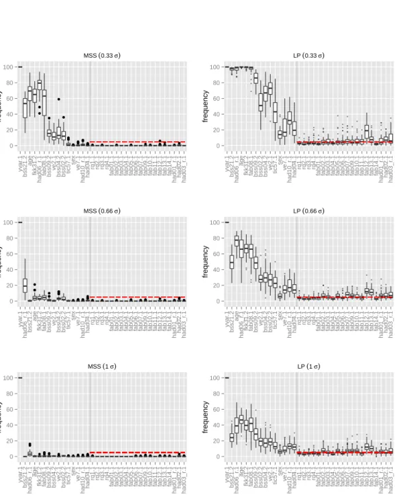
repetition and variable the percentage ofp-values smaller than 0.05 is counted. These percentages are displayed in boxplots, which are obtained from the outer repetitions. The results for MSS are given on the left, the results for LDPE on the right, the rows represent varying degrees of dispersion. Within each panel the results for the relevant predictors are shown on the left of the vertical line. On the right the results for a selection of irrelevant predictors is shown.

For the relevant variables the boxes represent the power. The order of the vari-ables is determined by the effect sizes, which were computed as the product of the true coefficients and the empirical standard deviations of the predictors, that is,

β_j∗·sd(x(j)_{), j ∈S}∗_{. As expected, the smaller the effect size, the lower the percentage}

of p-values smaller than 0.05. For higher dispersion the power drops drastically, ex-cept for the baseline-predictor. The power obtained for MSS indicate that for higher dispersion the relevant predictors cannot be detected.

For the irrelevant variables the percentage correspond to type-I-errors of every repe-tition. Its control at the 5% level is marked by the dashed horizontal line. The MSS p-values are rarely beneath 0.05 indicating that the error level is not kept. Actually, the construction of these method results most often in p-values placed on one. In contrast the type-I-errors of LDPE are spread at 5%. Except for single predictors with higher type-I-errors, which can be explained by correlations with relevant pre-dictors. In scenarios with decorrelated irrelevant predictors increased type-I-errors disappeared.

0 20 40 60 80 100 yv ar .1 bss21.2 age fkk31.2 had06_r .1 fab08.1 bss09.2 v e2.1 bss04.2 bss02.2 tic57.1 se x v e7.1 had10_r .1 had04.1 rq1.1 rq2.1 rq3.1 rq4.1

fab01.1 fab02.1 fab03.1 fab04.1 fab05.1 fab06.1 fab07.1 fab09.1 fab10.1 fab11.1 fab12.1 fab13.1 fab14.1

had01_r .1 had02.1 had03_r .1 frequency MSS(0.33 σ) 0 20 40 60 80 100 yv ar .1 bss21.2 had06_r .1 age fkk31.2 fab08.1 bss09.2 bss02.2 bss04.2 v e2.1 tic57.1 se x v e7.1 had10_r .1 had04.1 rq1.1 rq2.1 rq3.1 rq4.1

fab01.1 fab02.1 fab03.1 fab04.1 fab05.1 fab06.1 fab07.1 fab09.1 fab10.1 fab11.1 fab12.1 fab13.1 fab14.1

had01_r .1 had02.1 had03_r .1 frequency LP(0.33 σ) 0 20 40 60 80 100 yv ar .1 had06_r .1 bss21.2 age fkk31.2 fab08.1 bss09.2 v e2.1 bss04.2 bss02.2 tic57.1 se x v e7.1 had10_r .1 had04.1 rq1.1 rq2.1 rq3.1 rq4.1

fab01.1 fab02.1 fab03.1 fab04.1 fab05.1 fab06.1 fab07.1 fab09.1 fab10.1 fab11.1 fab12.1 fab13.1 fab14.1

had01_r .1 had02.1 had03_r .1 frequency MSS(0.66 σ) 0 20 40 60 80 100 yv ar .1 bss21.2 age had06_r .1 fkk31.2 fab08.1 bss09.2 v e2.1 bss04.2 bss02.2 tic57.1 se x v e7.1 had10_r .1 had04.1 rq1.1 rq2.1 rq3.1 rq4.1

fab01.1 fab02.1 fab03.1 fab04.1 fab05.1 fab06.1 fab07.1 fab09.1 fab10.1 fab11.1 fab12.1 fab13.1 fab14.1

had01_r .1 had02.1 had03_r .1 frequency LP(0.66 σ) 0 20 40 60 80 100 yv ar .1 bss21.2 had06_r .1 age fkk31.2 fab08.1 bss09.2 bss04.2 v e2.1 bss02.2 tic57.1 se x v e7.1 had10_r .1 had04.1 rq1.1 rq2.1 rq3.1 rq4.1

fab01.1 fab02.1 fab03.1 fab04.1 fab05.1 fab06.1 fab07.1 fab09.1 fab10.1 fab11.1 fab12.1 fab13.1 fab14.1

had01_r .1 had02.1 had03_r .1 frequency MSS(1 σ) 0 20 40 60 80 100 yv ar .1 bss21.2 had06_r .1 age fkk31.2 fab08.1 bss09.2 bss02.2 bss04.2 v e2.1 tic57.1 se x v e7.1 had10_r .1 had04.1 rq1.1 rq2.1 rq3.1 rq4.1

fab01.1 fab02.1 fab03.1 fab04.1 fab05.1 fab06.1 fab07.1 fab09.1 fab10.1 fab11.1 fab12.1 fab13.1 fab14.1

had01_r .1 had02.1 had03_r .1 frequency LP(1 σ)

Figure 1: Inner repetitions percentages of p-values smaller than 0.05 of relevant and irrelevant predictors using MSS (left column) and LDPE (right column) and varying degrees of outcome dispersion (rows).

LP (0.33 σ) LP (0.66 σ) LP (1 σ) 0.0 2.5 5.0 7.5 10.0 12.5 0.00 0.05 0.10 0.15 0.20 0.00 0.05 0.10 0.15 0.20 0.00 0.05 0.10 0.15 0.20 type−I−error frequency

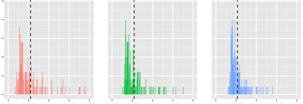
Figure 2: Empirical type-I-error of single hypothesis testing for each irrelevant pre-dictor for varying outcome dispersion on LDPE p-values.

4.2.1 Type-I-error

Figure2depicts to what extend a type-I-error of 5% is kept by LDPE. For each irrele-vant predictor the empirical type-I-error according to formula4.3has been calculated over all repetitions and is presented in histograms for varying outcome dispersion. While for higher dispersion the type-I-error spreads less, it is not symmetrically dis-tributed at a level of 0.05. Although their mean is slightly beneath 0.05 there exist some outlier till 0.2. Again this behavior disappears when irrelevant and relevant predictors are de–correlated. In this not depicted case the errors are spread narrowly at 0.05.

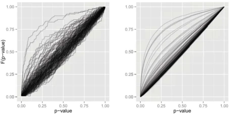
To conclude the results of p-values of irrelevant predictors, we provide their empirical cumulative distribution functions (ecdf) for each predictor in figure 3. Under the null hypothesis the distribution functions of the p-values should correspond to uniform distributions on the interval (0,1). In the left handed panel a distribution function for each predictor of one scenario repetition shows them spread around the diagonal of

0100 0123 0130 0143 5100 0100 0123 0130 0143 5100 6789 67 89 0100 0123 0130 0143 5100 0100 0123 0130 0143 5100 6789

Figure 3: Empirical cumulative distribution functions F(p-value) of LDPE p-values of irrelevant predictors. Functions for each predictor of a single repetition (left) and over all repetitions (right) for maximum outcome dispersion (1_·σˆLM).

the unit square, except for some concave functions of stronger correlated predictors. In the right handed panel an ecdf for each predictor over all inner repetitions shows nearly perfect diagonals. In the case of decorrelation they spread symmetrically and narrowly around the diagonal. The observation that almost all MSS p-values are placed at a value of one makes its presentation obsolete.

4.2.2 Empirical power

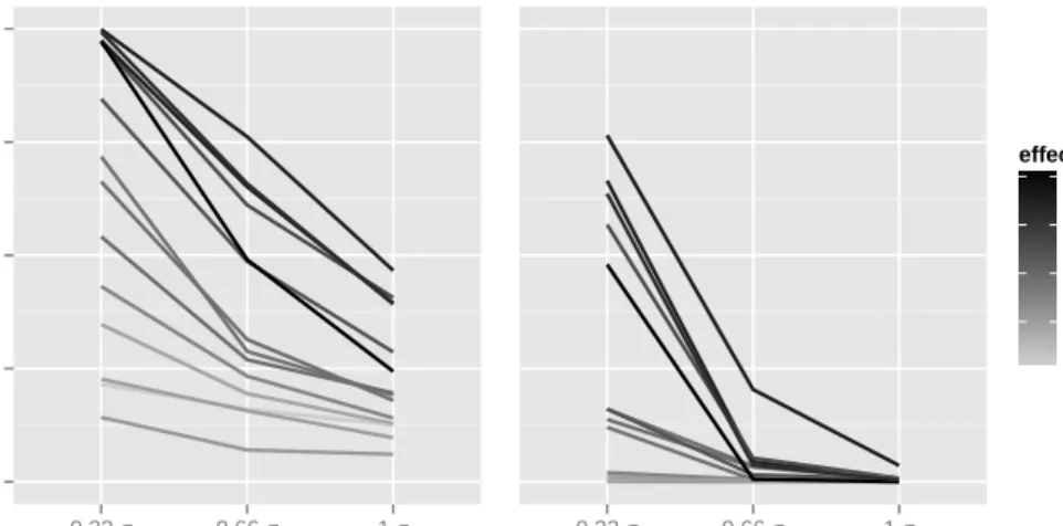
In a last step we analyse the power of single hypothesis testing for each relevant variable over all repetitions calculated according to formula4.2and depicted in figure

4for varying outcome dispersion and under consideration of effect sizes. The baseline-predictor stays withhold, having an distinctly higher effect size of 9.12 and keeping a constant power of one. For all other predictors the empirical probability of correctly rejecting the null hypothesis tends to zero for increasing outcome dispersion and

LP MSS 0.00 0.25 0.50 0.75 1.00 0.33 σ 0.66 σ 1 σ 0.33 σ 0.66 σ 1 σ outcome dispersion po w er 2.0 1.5 1.0 0.5 effect size

Figure 4: Empirical power values of single hypothesis testing for relevant predictors based on LDPE and MSS calculated p-values for varying outcome dispersion consid-ering different effect sizes.

smaller effect sizes. Especially for MSS it will not be possible to detect truly active variables.

4.2.3 Further scenarios

We increased the number of observations used for the simulations design matrices from n= 200 to n= 350 respectively the number of relevant predictors fromp∗ _{= 15}

to p∗ _{= 30, while keeping all other parameters of the main scenario unchanged. In}

the former variant we observed for LDPE slightly increased power values and a mean type-I-error of 0.053. In contrast, although we nearly doubled the data base the power increased only little, while the type-I-error stayed near zero. In the latter variant we added the next 15 predictors of the lasso path as relevant variables. The power values of LDPE generated p-values increased little for predictors common in both scenarios and type-I-errors spread stronger, with a total mean of 0.054.

4.2.4 Conclusion

In all we observed for LDPE p-values a type-I-error slightly above the requested value of 0.05. Outliers were caused by correlations with relevant predictors. For predictors with low effect sizes the power of hypothesis testing will be small, even reduced by higher outcome dispersion. In this study MSS seems an inappropriate method for generating p-values. The power of hypothesis testing seems very small and caused by construction of these method, error-rate is not keepable. Additionally MSS will get computational difficulties, if variables have to few different values, resulting in inestimable model coefficients. Depending on the number of considered predictors the computational costs and time for LDPE are far higher than for MSS.

5

Analysis of pain study

5.1

Method

According to our aim of a one-year prediction for pain intensity, we formulated a linear regression model. As possible predictors we used the baseline, psycho sociological items from the previously mentioned questionnaires and individual characteristics. In total the model contained 206 predictors, while 237 observations without missing values were available.

For the purpose of selecting the most relevant predictors via Lasso we applied the R-package penalized of Goeman (2010). We conduct the modeling procedure in two steps. In the first step variables are selected with the function profL1(), which generates coefficients for each predictor for a sequence of penalty values. At that we allow all predictors to be penalized and therefore selected, except the unpenalized control variables age, sex and center of survey. The optimal penalty strength is determined in the optL1()-function via 10-fold crossvalidation. In the second step we refit the coefficients of selected and unpenalized predictors in a linear regression model. This returns unbiased coefficients, in contrast to biased Lasso coefficients. LDPE generated p-values are opposed to those selected and not selected predictors and interpreted according to the findings of the simulation study.

5.2

Results

A detailed contentual description and interpretation of the Lasso-results is given in Wippert et al. (subm.). Therefore we focus upon the methodical aspects and

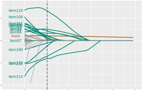
base item114 item82 item66 item119 item33 item130 item97 item100item93 item19 item190 item211 item117 item108 −4 −2 0 2 200 400 600 800 1000 1200 penalization strength λ β −coefficient

Figure 5: Coefficient paths with highlighted selected predictors for the crossvalidated optimal degree of penalization (vertical dashed line).

comparison to our simulation study. Coefficient paths of the Lasso selection are depicted in figure5representing for each predictor its against zero shrinking coefficient for increasing degree of penalization on an equidistant grid. An optimal degree of penalization calculated via 10-fold cross validation is marked by the vertical dashed line.

The application of Lasso shows the expected immense reduction of dimensionality of the coefficient vector from 206 to 15. Among those selected predictors, denoted in the plot, we find the marked baseline predictor of pain intensity named base. Its coefficient, compared to those of all other covariates, is very slowly shrunken to zero at an increasing degree of penalization.

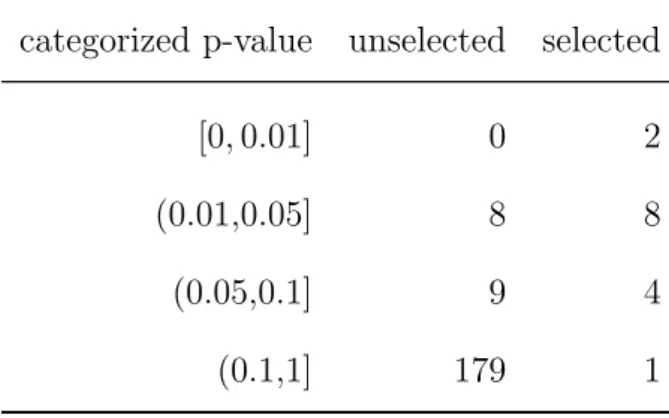
To the estimates for each selected predictor we added the p-value calculated by the LDPE ofZhang and Zhang (2014) based on the initial data set. While ten predictors

categorized p-value unselected selected

[0,0.01] 0 2

(0.01,0.05] 8 8

(0.05,0.1] 9 4

(0.1,1] 179 1

Table 1: Frequency of categorized LDPE p-values for unselected and selected predic-tors.

show a significant p-value at the error level of 5 %, the remaining five predictors have a non significant p-value. In table 1 we compare p-values of selected and unselected predictors in four categories. Besides the previously mentioned p-values of selected predictors eight of the remaining predictors received a significant p-value, too.

5.3

Conclusion

According to our simulation study we expect the small number of significant p-values caused by relevant variables with small effect sizes, compared to the effect size of the baseline predictor. As well as significant p-values of unselected predictors may be caused by correlations to selected predictors, keeping in mind that Lasso selects single covariates out of groups of correlated ones. The results of the simulation study for MSS generated p-values were confirmed in the analysis of the pain study. Except of the baseline predictor all predictors received a p-value of one making its presentation unnecessary.

6

Conclusion and discussion

In the past five years various approaches for inference in high-dimensional data set-tings have been proposed. There is missing experience regarding their performances and suitability for a broad application in practical data analysis. We analyzed p-values calculated by Multi Sample Splitting and the Low Dimensional Projection Estimator in a simulation study. The study was guided by our leading question of selecting one-year predictive psychometric items on back pain using the Lasso. Our model setting with n = 237 and p = 206 returned 15 selected predictors, including the baseline predictor. After selection We fitted their coefficients in a linear regression model, which results in invalid p-values of the usual t-statistic. The LDPE p-values based on Zhang and Zhang (2014) indicated significant effects for selected, as well as for unselected predictors.

The simulation study for LDPE and MSS p-values based on a setting of n = 200 and p = 174 and varying degrees of outcome dispersion. For LDPE p-values it showed strongly decreasing power for single hypothesis tests on active predictors for decreasing effect size and increasing outcome dispersion. Type-I-error calculations for tests on inactive predictors pointed out, that a level of 5% was kept on average. The level was exceeded by single correlated predictors to a type-I-error of 0.2.

In contrast the MSS calculated p-values showed no satisfying results and can not be recommended for our data setting. While in all settings the type-I-error for tests on inactive predictors almost always took a value of zero, power calculations failed those of LDPE. This behaviour is caused by a non stable predictor selection in the repetitions of MSS. It seems questionable for reliable p-values, to use only half of

available information for selection in a setting, where observations are rare at all. Restrictively we have to emphasize that our modeling framework is dominated by the baseline predictor, with a strong association to the pain outcome.

Finally the relationship between p-values based on tests for all covariates and the p values of the Lasso selected ones has to be further explored.

References

Airaksinen, O., Brox, JI., Cedraschi, C., Hildebrandt, J., Klaber-Moffett, J., Kovacs, F., Mannion, AF., Reis, S., Staal, JB., Ursin, H., and Zanoli, G. (2006). Chapter 4. European guidelines for the management of chronic nonspecific low back pain. European Spine Journal, 15, 192–300.

Bartholomew, K. and Horowitz, LM. (1991). Attachment styles among young adults: a test of a four-category model. Journal of Personality and Social Psychology,61, 226–244.

B¨uhlmann, P., Meier, L., and van de Geer, S. (2014). Invited discussion on ’a signifi-cance test for the lasso (Lockhart, R., Taylor, J., Tibshirani, R. J., and Tibshirani, R. (2014)). The Annals of Statistics, 42, 469–477.

Chatterjee, A., and Lahiri, S. (2010). Asymptotic Properties of the Residual Boot-strap for Lasso Estimators.Proceedings of the American Mathematical Society,138, 4497–4509.

Chatterjee, A., and Lahiri, S. (2011). Bootstrapping Lasso Estimators.Journal of the American Statistical Association, 106, 608–625.

Dezeure, R., B¨uhlmann, P., Meier, L., and Meinshausen, N. (2015). High-Dimensional Inference: Confidence Intervals, p-Values and R-Software hdi. Statistical Science,

30, 533–558.

Fan, J. and Lv, J. (2010). A Selective Overview of Variable Selection in High Dimen-sional Feature Space. Statistica Sinica, 20, 101–148.

Gesundheitsreport (2014). Risiko Rcken. Verffentlichungen zum Betrieblichen Gesundheitsmanagement der Techniker Krankenkasse,29, Hamburg.

Goeman, J. (2010). L1 Penalized Estimation in the Cox Proportional Hazards Model.

Biometrical Journal, 52, 70–84.

Groll, A. and Tutz, T. (2014). Variable selection for generalized linear mixed models by L (1)-penalized estimation. Statistics and Computing, 24, 137–154.

Hasenbring. M,, Hallner. D. and Rusu, AC. (2009). Fear-avoidance- and endurance-related responses to pain: development and validation of the Avoidance-Endurance Questionnaire (AEQ).European Journal of Pain, 13, 620–628.

Hemingway, H., Croft, P., Perel, P., et al. (2013). Prognosis research strategy (PROGRESS) 1: a framework for researching clinical outcomes.BMJ,346:e5595.

Herrmann, C., Buss, U. and Snaith, RP. (1995). Hospital Anxiety and Depression Scale - Deutsche Version (HADS-D). Manual.Hans Huber, Bern.

Hill, JC., Dunn, KM., Lewis, M., et al. (2008). A primary care back pain screening tool: identifying patient subgroups for initial treatment.Arthritis Rheum,59, 632– 641.

Hill, JC., Vohora, K., Dunn, KM., et al. (2010). Comparing the STarT back screening tools subgroup allocation of individual patients with that of independent clinical experts.Clin J Pain,26, 783–787.

Hingorani, AD., Windt, DA., Riley, RD., et al. (2013). Prognosis research strategy (PROGRESS) 4: stratified medicine research. BMJ,346:e5793.

Ibrahim, T., Tleyjeh, IM., and Gabbar, O. (2008).Surgical versus nonsurgical treat-ment of chronic low back pain: a meta-analysis of randomised trials. Int Orthop,

32, 107–113.

Janwantanakul, P., Sihawong, R., Sitthipornvorakul, E., and Paksaichol, A. (2015). A screening tool for non-specific low back pain with disability in office workers: A 1-year prospective cohort study.BMC Musculoskeletal Disorders, 16:298.

Javanmard, A., and Montanari, A. (2014). Confidence Intervals and Hypothesis Test-ing for High-Dimensional Regression. The Journal of Machine Learning Research,

15, 2869–2909.

Knight, K., and Fu, W. (2000). Asymptotics for Lasso-Type Estimators. The Annals of Statistics, 28, 1356–1378.

Krampen, G. (1991). Fragebogen zu Kompetenz- und Kontrollberzeugungen (FKK) (Inventory on Competence and Control Beliefs]). Hofgrefe, Gttingen.

Lechert, Y., Schroedter, J. and Lttinger, P. (2006). Die Umsetzung der Bildungsklas-sifikation CASMIN fr die Volkszhlung 1970, die Mikrozensus-Zusatzerhebung 1971 und die Mikrozensen 1976 2004. ZUMA-Methodenbericht, Mannheim.

(2016). Development of a yellow flag assessment tool for orthopaedic physical ther-apists: Results from the optimal screening for prediction of referral and outcome (OSPRO) cohort.The Journal of orthopaedic and sports physical therapy,46, 327– 343.

Lockhart, R., Taylor, J., Tibshirani, R. J., and Tibshirani, R. (2014a). A significance test for the lasso. The Annals of Statistics,42, 413–468.

Lockhart, R., Taylor, J., Tibshirani, R. J., and Tibshirani, R. (2014b). Rejoinder: ’A significance test for the lasso’. The Annals of Statistics, 42, 518–531.

Meier, L., Meinshausen, N., and Dezeure, R. (2014). hdi: High-Dimensional Inference. R package.

Meinshausen, N., Meier, L., and Bhlmann, P. (2009). p-Values for High-Dimensional Regression. Journal of the American Statistical Association - Theory and Methods,

104, 1671–1681.

Melloh, M., Roder, C., Elfering, A., Theis, JC., Muller, U., Staub, LP., Aghayev, E., Zweig, T., Barz, T., Kohlmann, T., Wieser, S., Juni, P., and Zwahlen, M. (2008). Differences across health care systems in outcome and cost-utility of surgi-cal and conservative treatment of chronic low back pain: a study protocol. BMC Musculoskelet Disord, 9:81.

Menezes Costa, LC., Maher, CG., Hancock, MJ., McAuley, JH., Herbert, RD., and Costa, LO. (2012). The prognosis of acute and persistent low-back pain: a meta-analysis. CMAJ, 184, E613–E624.

and Management of Psychological Risk Factors (Yellow Flags) in Patient With Low Back Pain: A Reappraisal. Physical Therapy, 91, 1–17.

Pfingsten, M., Leibing, E., Franz, C., Bansemer, D., Busch, O. and Hildebrandt, J. (1997). Erfassung der fear-avoidance-beliefs bei Patienten mit R¨uckenschmerzen: Deutsche Version des fear-avoidance-beliefs questionnaire (FABQ-D).Der Schmerz,

11, 387–395.

Pfingsten, M., Nagel, B., Emrich, O., Seemann, H. and Lindena, G. (2007). Deutscher Schmerz-Fragebogen - Handbuch: Deutsche Gesellschaft zum Studium des Schmerzes DGSS.

Riley, RD., Hayden, JA., Steyerberg, EW., et al. (2013). Prognosis Research Strategy (PROGRESS) 2: prognostic factor research. PLoS Med, 10:e1001380.

Schnorpfeil, P., Noll, A., Wirtz, P., Schulze, R., Ehlert, U., Frey, K. and Fischer, JE. (2002). Assessment of exhaustion and related risk factors in employees in the manufacturing industrya cross- sectional study. Int Arch Occup Environ Health,

75, 535–540.

Schultz, IZ., Crook, J., Berkowitz, J., Milner, R., and Meloche, GR. (2005). Predicting return to work after low back injury using the Psychosocial Risk for Occupational Disability Instrument: a validation study.J Occup Rehabil, 15, 365–376.

Schulz, P., Schlotz, W. and Becker, P. (2004).Trierer Inventar zum chronischen Stress (TICS). Hofgrefe, G¨ottingen.

Schwarzer, R. and Schulz, U. (2000). Berliner Social-Support Skalen. Berlin: Freie Universit¨at, Abteilung f¨ur Gesundheitspsychologie.

Statistisches Bundesamt (2010). Krankheitskosten in Mio. Euro f¨ur Deutschland. Ad-hoc-table. http://www. gbe-bund.de, April 30, 2014.

Tibshirani, R. (1996). Regression Shrinkage and Selection via the Lasso. Journal of the Royal Statistical Society – Series B (Methodological), 58, 267–288.

Traeger, A., Henschke, N., Hubscher, M., Williams, CM., Kamper, SJ., Maher, CG., Moseley, GL., and McAuley, JH. (2015). Development and validation of a screening tool to predict the risk of chronic low back pain in patients presenting with acute low back pain: a study protocol. BMJ open, 5(7):e007916.

Traeger, A., Henschke, N., Hubscher, M., Williams, CM., Kamper, SJ., Maher, CG., Moseley, GL., and McAuley, JH. (2016). Estimating the risk of chronic pain: De-velopment and validation of a prognostic model (PICKUP) for patients with acute low back pain. PLoS medicine, 13(5):e1002019.

Von Korff, M., Ormel, J., Keefe, FJ., and Dworkin, SF. (1992). Grading the severity of chronic pain. Pain, 50, 133–149.

Wasserman, L., and Roeder, K. (2009). High-Dimensional Variable Selection. The Annals of Statistics, 37, 2178–2201.

Wippert, PM., Puschmann, AK., Weiffen, A., Drielein, D., Arampatzis, A., Banzer, W., Beck, H., Schiltenwolf, M., Schmidt, H., Schneider, C. and Mayer, F. (subm.), Development of a Risk Stratification Index and a Risk Prevention Index for chronic low back pain in primary care. Focus: yellow flags (MiSpEx Network).

Zhang, C. and Zhang, S. (2014). Confidence intervals for low dimensional parameters in high dimensional linear models.Journal of the Royal Statistical Society – Series B (Methodological), 76, 217–242.