Bayesian Inversion and Inference of
Categorical Markov Models with
Likelihood Functions Including
Dependence and Convolution
Torstein Mæland Fjeldstad
Master of Science in Statistics
Supervisor: Karl Henning Omre, MATH
Department of Mathematical Sciences Submission date: June 2015
i
Abstract
A convolutional two-level Markov model is studied in this thesis. The bottom level con-tains a latent Markov chain, and given the variables, the middle concon-tains a latent Gaussian random field. We observe the second level through a convolution with additive Gaussian noise. Previously studied models are extended by including additional spatial correlation in the middle layer.
We propose two different approximations of the likelihood function, namely the truncation and projection approximation, of varying order. These approximate models are exactly assessed by the Forward-Backward algorithm.
Properties of various predictors are studied in different approximate posterior models. The predictors are seen to be stable with respect to an increase of the spatial correlation
in the response model. An increase of k, being the approximation order, is not seen to
have a great effect on the predictors.
The approximate posterior models are used as proposal densities in a Metropolis-Hastings algorithm to assess the correct posterior model, and we quantify the quality of each approximation by the acceptance rate. The acceptance rate is observed to be an increasing
function ofk. We observed higher acceptance rates when the proportion of the acquisition
convolution was high, relative to the spatial correlation. A high class response variance also increased the acceptance rate.
Estimation of the transition matrix, using the EM-algorithm and simulation based infer-ence, is found to be feasible under certain conditions. A univariate maximum marginal likelihood estimation of the model parameter in the Ricker acquisition convolution kernel is considered.
iii
Samandrag
I denne masteroppgåva studerer me ein konvolvert to-nivå Markov modell. Det første nivået er ei ikkje-observerbar Markovkjede, som definerer eit ikkje-observerbart Gaussisk stokastisk felt. Me observerer dette feltet gjennom ein konvolusjon, saman med Gaussiske feil. Modellen vår utvidar tidlegare studerte modellar ved å inkludere romleg korrelasjon på det midterste nivået.
Me føreslår to ulike approksimasjonar for likelihoodfunksjonen. Dei er baserte på høve-vis trunkering og projeksjon. Dei approksimative modellane kan evaluerast eksakt med framlengs-baklengs algoritmen.
Ulike prediktorar for den approksimative posteriorifordelinga er samanlikna, og me stud-erer eigenskapane deira under ulike modellføresetnader. Prediktorane er observert å vere nær uavhengig av romleg korrelasjon i responsmodellen, samt nær uavhengig av
approksi-masjonsordenen, k.
Dei approksimative modellane er nytta som forslagsfordelingar i ein Metropolis-Hastings
algoritme til å generere realisasjonar frå den sanne posteriorifordelinga.
Akseptanse-sannsynet er nytta som eit mål for å kvantifisere approksimasjonen. AkseptanseAkseptanse-sannsynet
er observert å auke saman medk. Approksimasjonane er sett å vere gode når konvolusjon
i observasjonsmodellen er stor, samanlikna med den romlege korrelasjonsfunksjonen. Ak-septansesannsynet er observert å auke dersom variansen i responsklassane vert auka. Parameterestimering av overgangsmatrisa ved hjelp av EM-algoritmen og simulering, er studert under visse føresetnader. Estimatet er sett å samsvare med den sanne overgangs-matrisa i gitte tilfelle. A priori kjennskap er sett å vere naudsynt, særskilt dersom dei ulike klassane overlappar kvarandre. Univariat optimalisering av marginal likelihoodfunksjonen er studert for ein Rickerfunksjon.
v
Acknowledgments
First of all, I would like to express my sincere gratitude to my supervisor, Professor Henning Omre, for his help and guidance during my work. His inputs and feedback has ensured my progress, and he has been very encouraging and supportive during my effort to complete my thesis.
I would also like to thank Assistant Professor Dario Grana at the University of Laramie, Wyoming, for his hospitality last fall.
Special thanks to my friends and fellow students for five enjoyable years.
I would also like to thank my family for their support during my stay in Trondheim. Finally, I would like to thank Torill for her continuous support.
Contents
1 Introduction 3 1.1 Outline of Notation . . . 3 1.2 Problem Description . . . 3 2 Probabilistic Model 7 2.1 Prior Model . . . 7 2.2 Likelihood Model . . . 9 2.2.1 Response Likelihood . . . 9 2.2.2 Acquisition Likelihood . . . 11 2.2.3 Gross Likelihood . . . 12 2.3 Posterior Model . . . 13 2.3.1 Related Models . . . 14 3 Posterior Assessment 17 3.1 Likelihood Approximations . . . 19 3.1.1 Truncation . . . 19 3.1.2 Projection . . . 20 3.1.3 Comparison of Approximations . . . 223.2 Assessment of the Approximate Posterior Model . . . 22
3.3 Assessment of the Correct Posterior Model . . . 25
4 Parameter Inference 29 4.1 Marginal Likelihood . . . 29
4.1.1 Approximate Maximum Marginal Likelihood . . . 29
4.1.2 Approximate Maximum Marginal A Posterior . . . 30
4.2 The Expectation-Maximization Algorithm . . . 32
4.3 Model Parameters . . . 33
4.3.1 Prior Model Parameters . . . 33
4.3.2 Response Model Parameters . . . 35
4.3.3 Parameters in the Acquisition Model . . . 36
5 MAP Case Studies 37 5.1 Model Specification . . . 38
5.1.1 Reference Case . . . 39
5.1.2 Apparent Convolution Kernel . . . 47
5.1.3 Apparent Convolution Width . . . 51
5.1.4 Variances in Response Model . . . 54
5.1.5 Spatial Correlation Response Model . . . 57
5.2 Closing Remarks . . . 60
6 Assessment of the Transition Matrix 61
6.1 High Reflector Points . . . 61 6.1.1 Model Specification . . . 61 6.1.2 Results . . . 64 6.2 Ordered Profile . . . 68 6.2.1 Model Specification . . . 68 6.2.2 Results . . . 70 6.3 Closing Remarks . . . 73
7 Case Study: Seismic Inversion 75 7.1 Model Specification . . . 76
7.2 Results . . . 78
7.2.1 MAP Prediction . . . 78
7.2.2 Simulation from the Response Model . . . 80
7.2.3 Estimation of the Transition Matrix . . . 80
7.2.4 Estimation of the Acquisition Convolution Kernel . . . 84
7.3 Closing Remarks . . . 84
8 Conclusions and Future Work 85 Appendices 91 A Probability Distributions 93 A.1 Gaussian Distribution . . . 93
A.2 Dirichlet Distribution . . . 94
Chapter 1
Introduction
This chapter introduces the necessary notation and defines the variables of interest. We relate our variables of interest to seismic inversion, and introduce briefly the concepts of Bayesian inversion. A short introduction to point predictors and parameter inference is given.
1.1
Outline of Notation
A generic vector of length t is denoted by a = (a1, . . . , at)>, and we define a−k =
(a1, . . . , ak−1, ak+1, . . . , at)
>
. We denote a generic(t×s)-matrix byA, where the identity
matrix is denoted by I. Element (i, j) in A is denoted by [A]ij. The indicator function,
1{A}, is defined to be equal to 1 if A is true, and 0 otherwise.
A random variable x with sample space Ωx, is assumed to be distributed according to a
generic probability distributionp(x). Ifxis discrete we refer top(x)as a probability mass
function, and if x is continuous we refer to it as a probability density function. Relevant
probability distributions are given in Appendix A.
1.2
Problem Description
We consider a random field defined on D ∈R, discretized onto a lattice LD :{1, . . . , N}.
This can for example represent a vertical profile through a geological unit, such as a seismic profile penetrating the subsurface.
Our variable of interest is a vector κ = (κ1, . . . , κNκ)
>
, where we for notational ease
let Nκ = N. For n = 1, . . . , N, each κn represents a nominal or ordinal class with
κn ∈Ωκ :{1, . . . , K}. This could for example represent the lithology/fluid-characteristics,
such as {shale, sand/brine, sand/oil, sand/gas}. The set ΩN
κ is defined to be the KN
possible configurations of κ, which in practice usually is an extremely large set.
We observe a continuous vectord= (d1, . . . dNd)
>
, whereNd≤N in most situations. In for
example reservoir modelling, the observations may contain information from seismic data, well-logs or production history data. We only consider one-dimensional observations, i.e.
dn ∈Rforn= 1, . . . , Nd, but it is possible to extend to multivariate observations. Buland
and Omre (2003) discuss how the latter can be modeled with seismic amplitude versus offset (AVO) data. The elastic properties P-wave velocity, S-wave velocity and density are modeled utilizing the fact that the seismic reflection amplitude depends on the contrast of the material properties and reflection angles at each point of reflection.
Our goal is to assess [κ|d], i.e. classify the latent categorical vector based on the obser-vations. We operate in a probabilistic framework,
[κ|d]∼p(κ|d), (1.1)
where the random variable [κ|d]is distributed according to the probability mass function
p(κ|d). A major benefit with assessing Eq. (1.1) in a probabilistic framework is that we
can provide point predictions with uncertainty statements.
We assess Eq. (1.1) in a Bayesian framework, where we assign a prior model, p(κ), to
κ. The prior model represents a priori knowledge of κ, for example the expected waiting
time in each class. Correspondingly, we define an observation model, [d|κ] ∼ p(d|κ).
Since d is given, andκ is the unknown variable,p(d|κ) is in fact a likelihood function as
it need not be normalized with respect to κ. The posterior model for [κ|d]is assessed by
using Bayes’ theorem,
p(κ|d) = p(d|κ)p(κ)
p(d) . (1.2)
The posterior modelp(κ|d)is referred to as the solution to a Bayesian inversion problem.
Being a function of κ, the posterior is seen to be proportional to the likelihood times the
prior. The probabilistic characteristics of [κ|d] are captured in the posterior. We may
generate realizations from the posterior model.
We operate in a predictive setting, and want to make predictions with the associated un-certainty statements. We choose the maximum a posteriori probability (MAP) predictor as our predictor since the predictor is contained in the discrete sample space. This need not be true for the posterior mean or median. The MAP predictor is defined as
ˆ
κ= arg max
κ
{p(κ|d)}. (1.3)
Assessment of the MAP predictor constitutes a hard problem since it requires evaluation
of KN possible configurations of κ. An alternative is therefore to consider the marginal
MAP (MMAP) predictor,
ˆ ˆ κ= ˆ κn= arg max κn {p(κn|d)};n ∈ LD . (1.4)
Uncertainty statements can be made by computing the marginal probabilities for each class. In practice the predictors differ from the posterior median, which is dependent on
the labeling of κ.
Both the prior and likelihood models are dependent on unknown model parameters. We
denote themθ = (θp,θl), where respectivelyθp and θl are the prior and likelihood model
parameters. To make the dependence on model parameters clear, we may rewrite Eq. (1.2) as
p(κ|d;θ) = p(d|κ;θl)p(κ;θp)
p(d;θ) . (1.5)
The maximum marginal likelihood estimator, ˆθ, and the normalization constant p(d;θ)
are closely related since
ˆ
θ= arg max
θ
1.2. PROBLEM DESCRIPTION 5 Eq. (1.6) can for example be maximized using the expectation-maximization (EM) algo-rithm. Due to the spatial dependency and possible local optima, the optimization might be complex to perform.
It is also possible to impose prior knowledge onθ, by assumingθ∼p(θ). The assessment
of θ is then cast into a Bayesian inference setting. Then we are able to generate
poste-rior realizations from p(θ|d). The latter can be done using Markov chain Monte Carlo
simulation.
In Chapter 2 we introduce the current model in greater detail. We specify a convolu-tional Markov model through a prior, response and acquisition model, and deduce the
posterior model. We study various k-th order approximations of the posterior model in
Chapter 3, which can be assessed by the Forward-Backward algorithm. In Chapter 4 we study various model parameter estimation techniques, and discuss how the various model parameters can be assessed efficiently. Chapter 5 contains a thorough study of MAP predictors for various likelihood approximations. We compare various distance measures between the correct posterior model and the approximate posterior model. In Chapter 6 we have included two case studies where we estimate the transition matrix. In Chapter 7 a synthetic seismic test study is included. Finally, a summary of our findings are given in Chapter 8.
Chapter 2
Probabilistic Model
The posterior model,
p(κ|d;θ) = p(d|κ;θl)p(κ;θp)
p(d;θ) , (2.1)
is proportional to the likelihood model times the prior model. These models are presented in greater details in the following chapter. The prior is assumed to follow a first order
Markov chain, and we assume that each observation, dn, depends on κ. We relate the
model assumptions to a hidden Markov model, as defined in Cappe et al. (2005), and Frühwirth-Schnatter (2006). We specify a Gauss-linear acquisition likelihood model, and introduce a latent response likelihood model. The response likelihood model can for exam-ple represent the log-physics response in well-log data. From the acquisition and response likelihoods we define the gross likelihood, and study the apparent convolution kernel. In the following chapter we omit the model parameter dependence to ease notation.
2.1
Prior Model
Let κ= (κ1, . . . , κN) be a first order Markov chain, i.e. it satisfies
p(κn|κn−1, . . . , κ1) = p(κn|κn−1) (2.2)
for n = 2, . . . , N. The transition (K ×K)-matrix is defined as Pκ = [pij]i,j∈Ωκ, where
pij =p(κn =j|κn−1 =i), is identical for alln. We assume a stationary Markov chain, i.e.
the transition probabilities are independent of n, and has a stationary distribution given
by
ps(κ) =Pκ ps(κ). (2.3)
Since κ1 ∼ ps(κ1), it follows that κ2 ∼ Pκ ps(κ1), κ3 ∼ P2κ ps(κ1) an so on. Hence,
Eq. (2.3) gives the marginal distributions as
p(κn) = ps(κn). (2.4)
Thus, the marginal probability mass functions are identical for n = 1, . . . , N. We define
the prior model as
p(κ) = N Y n=1 p(κn|κn−1), (2.5) 7
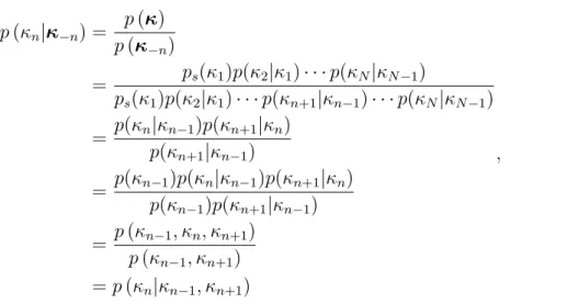
where p(κ1|κ0) =ps(κ1) for notational ease. Since p(κn|κ−n) = p(κ) p(κ−n) = ps(κ1)p(κ2|κ1)· · ·p(κN|κN−1) ps(κ1)p(κ2|κ1)· · ·p(κn+1|κn−1)· · ·p(κN|κN−1) = p(κn|κn−1)p(κn+1|κn) p(κn+1|κn−1) = p(κn−1)p(κn|κn−1)p(κn+1|κn) p(κn−1)p(κn+1|κn−1) = p(κn−1, κn, κn+1) p(κn−1, κn+1) =p(κn|κn−1, κn+1) , (2.6)
each κn is conditionally independent of κ1, . . . , κn−2, κn+2, . . . , κN given κn−1 and κn+1.
In Fig. 2.1 the correlation structure of a first order Markov chain is given. Indeed, the first order Markov chain is a simple one dimensional Markov random field. Informally,
the latter is defined for a random variable x on a latticeS, with a neighbouhood system
δs, if for all s∈ S
p(xs|x−s) =p(xs|xt;t ∈δs). (2.7)
In our case, S is one dimensional and identical to LD, where for each s ∈ S, δs = (s−
1, s+ 1), except at the boundary.
κ
1κ
2 . . .κ
N−1κ
NFigure 2.1: Graphical model of the correlation structure of a first order Markov chain. The first order Markov assumption ensures a forward spatial coupling in the prior model, however also the time-reversed chain defined by
p(κ) =p(κN)p(κN−1|κN)p(κN−2|κN−1, κN). . . p(κ1|κ2, . . . , κN), (2.8)
is a first order Markov chain since
p(κn|κn+1, . . . , κN) = p(κn)× QN i=n+1p(κi|κi+1) p(κn+1)×QNi=n+2p(κi|κi+1) = p(κn)p(κn+1|κn) p(κn+1) =p(κn|κn+1) . (2.9)
The prior model for the time-reversed Markov chain is given as
p(κ) =ps(κN)× N−1
Y
n=1
2.2. LIKELIHOOD MODEL 9 If the stationary distribution is uniform, then the time-reversed Markov chain and original Markov chain are identically distributed.
The stationary, first-order Markov chain assumption is not critical in our approach, in fact any non-homogeneous higher order Markov chain can be used.
The prior model is completely specified by the transition matrix,Pκ, thus the prior model
parameters are given as θp ={Pκ}. There are K×(K −1)unknown model parameters
in the prior model since each row has to sum to unity.
2.2
Likelihood Model
We assume a gross likelihood model by introducing a latent continuous random field
r = (r1, . . . , rN)>, where rn ∈ R for n = 1, . . . , N, as in Rimstad and Omre (2013), and
Lindberg and Omre (2014a). We assume [d,κ] to be conditionally independent given
r, i.e. r can be thought of as a bridge between κ and d, since we assume p(d,r|κ) =
p(d|r)p(r|κ). The likelihood models are referred to as the response model, [r|κ], and the
acquisition model, [d|r]. The gross likelihood model is given as
p(d|κ) =
Z
RN
p(d|r)p(r|κ) dr. (2.11)
The latent fieldrcan for example represent the logarithm of the elastic material properties,
such as pressure wave velocity, shear wave velocity and density. Experience from seismic
profiles indicates that r is a smooth field with spatial correlation. Therefore, we do not
assume the elements of r to be conditionally independent givenκ, as studied in Rimstad
and Omre (2013), and Lindberg and Omre (2014a).
We consider only so called Gauss-linear likelihood models, i.e. likelihood models that are linear in the modeling variable with additive Gaussian errors.
The gross likelihood depends on a vector of model parametersθl = (θlr,θla), whereθlr and
θla are respectively the model parameters in the response and acquisition likelihood.
2.2.1
Response Likelihood
We define the following response model,
[r|κ] =µr|κ+er|κ, (2.12)
where µr|κ is a N-vector with the mean and er|κ is a N-vector with errors. The
error-vector er|κ is assumed to be Gaussian with zero mean and covariance (N ×N)-matrix
Σr|κ. The response likelihood is thus given as
p(r|κ) = φN r;µr|κ,Σr|κ
. (2.13)
We assume the response likelihood to be stationary having mean and variance equal to µrn|κn = P κ0∈Ω κµr|κ0 ×1{κ 0 =κ n} σ2 rn|κn = P κ0∈Ω κσ 2 r|κ0 ×1{κ0 =κn} for n= 1, . . . , N, (2.14)
where µr|κ0 = µr|κ0 1, . . . , µr|κ 0 K > and σ2r|κ0 = σ2r|κ0 1, . . . , σ 2 r|κ0 K > . That is, µr|κ = µr1|κ1, . . . , µrN|κN >
. The covariance matrix is decomposed as
Σr|κ=Σσr|κΣ
ρ
r|κΣ
σ
r|κ, (2.15)
where Σσr|κ = diag(σr1|κ1, . . . , σrN|κN) is a diagonal standard deviation (N ×N)-matrix.
The (N ×N)-matrix with correlations, Σρr|κ, is defined from the correlation function,
ρr|κ(h). We propose a correlation model for the random field, r, with a dependent mode
process. The dependent mode process represents a common spatial correlation function for all mode processes,
[Σρr]n,n+h =ρr(h). (2.16)
With a dependent mode process the residuals in the Gauss mode processes are correlated. More complicated spatial correlation functions are possible, and include among others a switching process between different independent mode processes defined through an indicator function.
The marginal density of r is studied in greater detail, since its distributional properties
are used to propose an approximation to the response likelihood. Indeed,
p(r) = X
κ∈ΩN
κ
φN(r|κ)p(κ) (2.17)
is a multivariate Gaussian mixture with marginal distributions,
p(rn) =
X
κ∈Ωκ
φ1(rn|κ)ps(κ) for n = 1, . . . , N, (2.18)
being identical Gaussian mixtures.
A graphical representation of the current response model is given in Fig. 2.2, where the arrows show the correlation structure in the prior and response models.
κ
1κ
2 . . .κ
N−1κ
Nr
1r
2 . . .r
N−1r
NFigure 2.2: Graphical model of the current response likelihood with the spatial correlation structure.
We assume the correlation function, ρr(h), to be parametrized by a truncation range, aρ,
and ψρ, being the functional representation of ρr(h). Therefore, Σρr is a band-diagonal
matrix with bandwidth 2aρ+ 1. The response likelihood depends on model parameters
θlr =
µr|κ0,σr2|κ0, aρ,ψρ
. Indeed, the marginal Gaussian mixtures in Eq. (2.18) are defined by the conditional their respective conditional mean and variance.
2.2. LIKELIHOOD MODEL 11
2.2.2
Acquisition Likelihood
The acquisition model represents the observational procedure, describing the data collec-tion procedure. This can for example be either local averages, some exact observacollec-tions, or relative contrasts. We define the acquisition model to be a linear model,
[d|r] =Hr+ed|r, (2.19)
whereHis a general acquisition(Nd×N)-matrix, anded|ris aNd-vector with independent
error. The acquisition matrix may have Nd smaller, larger, or equal to N, but in most
cases Nd ≤N.
The acquisition likelihood is specified to be Gauss-linear, i.e. we assumeed|rto be additive,
independent ofrand Gaussian, more specifically with zero mean and covariance(Nd×Nd)
-matrix Σd|r=σd|r2 I. Hence, p(d|r) = φNd d;Hr, σ 2 d|rI . (2.20)
For a fixed observational matrix H, the acquisition likelihood is assumed to only depend
on a parameterσ2d|r, being the observational error for each observation. The observational
matrix, H, is completely general, and may be a convolution, selection, or mixed operator.
We will, however, consider only convolution operators.
A convolution arises naturally as a result of the dispersion of, for example, a physical
wavelet. A convolution is a local smoothness operator which makesdnnot only dependent
on rn, but also the neighbours of rn. In signal processing a convolution kernel is often
used, since it can represent smooth functions in an efficient way.
We denote our acquisition convolution(N×N)-matrix byH=W, where the acquisition
convolution kernel w is centered at the diagonal inW. We only consider symmetric and
stationary kernels, i.e. acquisition convolution kernels which are identical for alln, except
at the boundary. As Lindberg and Omre (2014a), we propose to truncate every element. Thus, each internal-node can be written as a sum,
dn = aw X
i=−aw
wirn+i+en for n= 1, . . . , N. (2.21)
Popular choices of acquisition convolution kernels are the Gaussian, the powered expo-nential, and Ricker wavelet, which we discretize and truncate on a grid. The truncation
reduces W to a band-diagonal matrix with bandwidth 2aw+ 1.
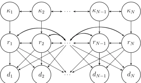
A graphical representation of the convolved acquisition likelihood, together with the prior and response models, is given in Fig. 2.3. We assume the acquisition
convolu-tion kernel to be parametrized by ψw. Thus, the acquisition likelihood is defined by
θla =
aw,ψw, σd|r2
.
In for example seismic inversion the convolutional matrix W can be used together with
a differential matrix, D, and a matrix A with the angle-dependent weak Aki-Richards
coefficients creating a mixed model, H = WAD. We refer to Buland and Omre (2003)
κ
1κ
2 . . .κ
N−1κ
Nr
1r
2 . . .r
N−1r
Nd
1d
2 . . .d
N−1d
NFigure 2.3: Graphical model of the current convolved model.
2.2.3
Gross Likelihood
We study the gross likelihood model, [d|κ], in Eq. (2.11) in greater detail. As both
our response and acquisition likelihood models are assumed to be Gauss-linear, the gross model
[d|κ] =W µr|κ+er|κ
+ed|r, (2.22)
is also Gauss-linear. Thus, the gross likelihood is
p(d|κ) = φNd d;Wµr|κ,WΣr|κW > +σ2d|rI =φNd d;µd|κ,Σd|κ . (2.23)
As seen in Eq. (2.23), µd|κ is only dependent on the acquisition convolution kernel and
not the spatial correlation function ρr(h). Since each dn appear as a weighted sum of
r, a short range acquisition convolution kernel ensures each dn to be a good read of rn.
We denote this the ’shoulder effect’, since a small aw ensures that each observation dn,
determined by rn and its neighbours, appears as a distinct shoulder ind.
In general, the covariance matrix depends on the band matrices W and Σρr. Therefore,
also WΣr|κW
>
+σ2
d|rI is a band matrix. It can be verified that WΣr|κW
>
in general results in coloured noise. We introduce the concept of an apparent convolution kernel, being the observed convolutional effect. Clearly, it is possible to fix the covariance matrix,
Σd|κ, and vary W and Σρr accordingly. Therefore, the effect is either from the spatial
correlation in the response model, or the from the acquisition convolution kernel, or both. Since
WΣr|κW
>
=Σσr|κWΣρrW>
Σσr|κ, (2.24)
we define the apparent convolution kernel as
WA =WΣρr1/2. (2.25)
The name apparent convolution refers to the observed convolution effect through the data.
If Σρr1/2 and W are parametrized by second order exponentials, then also the apparent
2.3. POSTERIOR MODEL 13
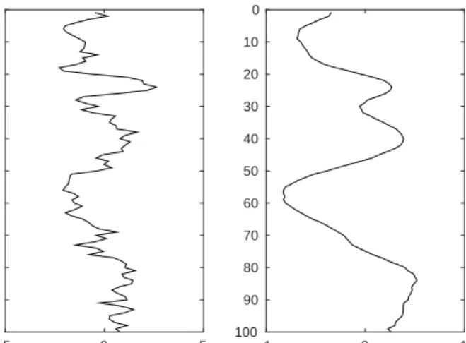
In Fig. 2.4 we have simulated a latent field, κ, and generated two set of observations
from posterior models with identical posterior covariance matrix. If WA = Σρr1/2, the
observation appears to have distinct shoulders. On the other hand, if WA = W the
observations are smoothed, and the small-scale variability is lost. We have therefore reason to expect that classification of the reference profile is an easier problem if most of the apparent convolution kernel results from the spatial correlation function.
5 10 20 30 40 50 60 70 80 90 100 WA = ' r ; 0 10 20 30 40 50 60 70 80 90 100 WA = W 0 10 20 30 40 50 60 70 80 90 100
Figure 2.4: Comparison of observed data with fixed apparent convolution. Left: Reference
profile. Middle: Apparent convolution kernel equals correlation function, Σρr = WA.
Right: Apparent convolution kernel equals acquisition convolution kernel, W=WA.
Finally, the gross likelihood model is defined by the joint set of model parameters,
θl = (θlr,θla) = µr|κ0,σ2r|κ0, aρ,ψρ, σd|r2 , aw,ψw .
2.3
Posterior Model
As we have seen in Eq. (1.2), the posterior model is given as
p(κ|d) = const×φNd d;Wµr|κ,WΣr|κW > +σ2d|rI× N Y n=1 p(κn|κn−1), (2.26)
where the normalizing constant is given as
const = X κ0∈ΩN κ φNd d;Wµr|κ0,WΣr|κ0W>+σ2d|rI × N Y n=1 p(κ0n|κ0n−1) −1 . (2.27)
Calculating the normalization constant, p(d), requires evaluating a sum including KN
permutations of κ. It is therefore computationally infeasible to evaluate Eq. (2.26) in
general. In practice the covariance matrix, WΣr|κW
>
+σ2
d|rI, is a band matrix with
band width at most 4aw+ 2aρ+ 1. Note that if W and Σr|κ are diagonal, then also the
covariance matrix in Eq. (2.26) is diagonal.
A r-th order factorial form function is defined to be
f(x1, . . . , xn) = n
Y
i=r+1
fi(xi−r, . . . , xi), (2.28)
which we denote a lag-rmodel forr < n. In practicef could be a likelihood function, such
that f is a product of fi-s, being likelihood approximations. The factorial form model
is related to the conditional independence structure in a model. A lag-r model defines a
Markov random field with the neighbourhood determined by δi = {i−r, . . . , i+r} for
node i. Independent xi-s corresponds to a lag-0 model, where one of the most studied
lag-0models is the hidden Markov model.
Our aim is to propose an approximation such that our posterior model, p(κ|d), is on
a lower order factorial form, and therefore a Markov random field. The approximate posterior model can then be exactly assessed, using the Forward-Backward algorithm. We need not approximate our prior model since it is already on factorial form. Our approximation extends previously studied models.
2.3.1
Related Models
The spatial coupling in [r|κ] makes our response likelihood model different from the one
studied in Rimstad and Omre (2013), and Lindberg and Omre (2014a). They assumed a
hidden Markov model for [r|κ], hence their response likelihood is on factorial form
p(r|κ) = N Y n=1 φ1 rn;µr|κ0 n, σ 2 r|κ0 n . (2.29)
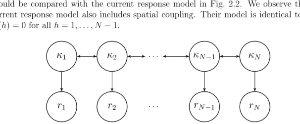
The response model studied in Rimstad and Omre (2013) is presented in Fig. 2.5, and should be compared with the current response model in Fig. 2.2. We observe that the current response model also includes spatial coupling. Their model is identical to our if
ρr(h) = 0 for all h= 1, . . . , N −1.
κ
1κ
2 . . .κ
N−1κ
Nr
1r
2 . . .r
N−1r
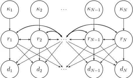
N2.3. POSTERIOR MODEL 15 The current model also extends the Bernoulli-Gaussian model presented in Cheng et al. (1996), which only allows one-sided convolution. Compared to the current model, no spatial dependence is assumed in their prior and response models. A graphical model of the Bernoulli-Gaussian model is given in Fig. 2.6. In the Bernoulli-Gaussian model we
can not enforce any prior spatial dependence in κ.
κ
1κ
2 . . .κ
N−1κ
Nr
1r
2 . . .r
N−1r
Nd
1d
2 . . .d
N−1d
NFigure 2.6: Graphical model of the Bernoulli-Gaussian model presented in Cheng et al. (1996).
Finally, we present the Gaussian mixture model by Grana and Della Rossa (2010), and
later formalized by Amaliksen (2014). Instead of focusing on κ, they studied the
poste-rior p(r|d) by assigning a prior p(r) to r. They studied the continuous elastic material
properties, not the hidden categorical field, κ, representing the lithofacies. A graphical
model of their model is shown in Fig. 2.7. Note that they included no spatial dependence
in κ.
κ
1κ
2 . . .κ
N−1κ
Nr
1r
2 . . .r
N−1r
Nd
1d
2 . . .d
N−1d
NFigure 2.7: Graphical model of the Gaussian mixture model presented in Grana and Della Rossa (2010).
The imposed spatial correlation and multimodality are observed features from drilled
multivariate Gaussian mixture model in the current model. Moreover, since p(r|d) = [p(d)]−1p(d|r)p(r) = [p(d)]−1×X κ p(d|r)p(r|κ)p(κ) = X κ∈ΩN κ p(d|r,κ)p(r|κ)p(κ) [p(κ,d)]−1p(κ,d) [p(d)]−1 = X κ∈ΩN κ p(r|d,κ)p(κ|d) , (2.30)
also the posterior [r|d]is a multivariate Gaussian mixture model. In fact, Eq. (2.30) is a
mixture in general for arbitrary densitiesp(κ), p(r|κ)andp(d|r). If we use known results
for Gaussian models, it follows that
p(r|d,κ) = φN r;µr|d,κ,Σr|d,κ , (2.31) where µr|d,κ=µr|κ+Σr|κW > WΣr|κW > +σd|r2 I −1 d−Wµr|κ Σr|d,κ=Σr|κ−Σr|κW> WΣr|κW>+σd|r2 I −1 WΣr|κ . (2.32)
If we have the posteriorp(κ|d), then we also have the posteriorp(r|d). We therefore only
focus on assessing p(κ|d).
As we have seen, our current model generalizes the models presented here. It is possible to extend our model by assuming coloured noise in the acquisition likelihood. However, the convolution impose coloured noise in the posterior covariance matrix. Therefore, we do not choose to assume a more complicated acquisition likelihood model. The prior model,
p(κ), may also be extended to a higher order Markov chain or a non-stationary Markov
Chapter 3
Posterior Assessment
The posterior model,
p(κ|d) = p(d|κ)p(κ)
p(d) , (3.1)
is computationally infeasible because of the normalization constant, p(d). We propose to
approximate the posterior model such that it can be written on factorial form, and hence be efficiently evaluated by the Forward-Backward algorithm. The simplest factorial form
approximation of Eq. (3.1), corresponding to k = 1, is
p(κ|d) =
QN
n=1p(d|κn)p(κn|κn−1)
p(d) , (3.2)
where the likelihood is factorized into single-site dependent factors. If we rewrite Eq. (3.2), we have p(κ|d) =p(κ1|d)× N Y n=2 p(κn|κn−1, . . . , κ1,d) =p(κ1|d)× N Y i=2 p(κn|κn−1,d). (3.3)
Indeed, the last equality in Eq. (3.3) holds since
p(κn|κn−1, . . . , κ1,d)∝p(κ1, . . . , κn|d) ∝ n Y i=1 p(d|κi)p(κi|κi−1) ∝p(d, κn|κn−1) ∝p(κn|κn−1,d) . (3.4)
Hence, κn depend only on d, κ1, . . . , κn−1 through κn−1 and d. Therefore, Eq. (3.3)
constitutes a first order non-stationary Markov chain. The posterior transition proba-bilites being conditional on the observations are however no longer a homogenous Markov chain.
For higher orderkapproximations, letκ(nk) = (κn−k+1, . . . , κn)be thek-th order state. Our
previous first order Markov chain is now rephrased as a k-th order Markov chain,
κ(k) = (κ1, . . . , κk), . . . ,(κN−k+1, . . . , κN)
, (3.5)
with a transition (Kk×Kk)-matrix, P(k)
κ . The elements are given as
pκ(nk)|˜κn(k−)1=p(κn|˜κn−1)× k−1 Y i=1 1{κn−k+i = ˜κn−k+i}. (3.6) 17
In order for the model to be consistent, the (k−1) top mode labels inκ(nk−)1 must equal
the (k−1) bottom mode labels in κ(nk). Therefore, we need not store the full transition
matrix Pκ(k). Similarly, pκn|˜κ (k) n−1 = X κ(nk−−11) pκ(nk)|˜κ(nk−−11) =p(κn|˜κn−1) X κ(nk−−11) k−1 Y i=1 1{κn−k+i = ˜κn−k+i} =p(κn|˜κn−1) , (3.7)
since there is only one κ(nk−−11) such that Qk−1
i=1 1{κn−k+i = ˜κn−k+i} = 1. Indeed, the prior p κ(k)= N Y n=k pκ(nk)|˜κ(nk−)1= N Y n=k k−1 Y i=1 1{κn−k+i = ˜κn−k+i} ! ×p(κn|˜κn−1), (3.8)
is still defined by the transition matrix Pκ.
Our likelihood approximation is inspired by Rimstad and Omre (2013), i.e. we seek a likelihood approximation on factorial form,
p(k) d|κ(k) = N Y n=k p(k) d|κ(nk) . (3.9)
This is of the same form as for k= 1, hence the likelihood approximations presented later
are valid for all k. If we combine Eq. (3.8) and Eq. (3.9), we can approximate Eq. (3.1)
with p(k) κ(k)|d = const× N Y n=k p(k) d|κ(nk)pκn(k)|κ(nk−)1, (3.10) where pκ(kk)|κk(k−)1 = ps
κ(kk) for notational ease. Thus, Eq. (3.10) is a k-th order
Markov chain with respect to κ(nk). The approximate posterior model in Eq. (3.10) is on
lag-(k−1) factorial form. The approximate posterior model is given as
p(k)(κ|d) = const×
N
Y
n=k
p(k) d|κ(nk)pκn(k)|κ(nk−)1, (3.11)
and is a factorial form model of lag-(k−1)for k ≥2.
We present two different likelihood approximations top(k)d|κ(k)
n
, namely the truncation and projection approximation. The Forward-Backward algorithm is derived in Section 3.2.
In Section 3.3 the correct posterior model, p(κ|d), is assessed using the approximate
3.1. LIKELIHOOD APPROXIMATIONS 19
3.1
Likelihood Approximations
We define two different likelihood approximations to Eq. (3.9), namely the truncation and
projection based approximations. Define thek-th order truncationsr(tk) = (rt−k+1, . . . , rt)
>
and d(tk) = (dt−k+1, . . . , dt)
>
for n = k, . . . , N. In both approximations we need the
marginal versions of p(r|κ), and we approximate the acquisition likelihood, p(d|r), by
either truncation or projection. We present the marginal response likelihoods, since they are identical for both approximations.
The response model, [r|κ], is Gaussian by assumption, hence from marginalization also
[r(nk)|κ] forn =k, . . . , N are Gaussian. The mean, µr(k)
n |κ, and covariance matrix, Σr
(k)
n |κ,
are found by extracting the appropriate rows and columns from µr|κ and Σr|κ. By
con-ditional independence it follows that
p r(nk)|κ=p r(nk)|κ(nk), κ1, . . . , κn−k, κn, . . . , κN
=p r(nk)|κ(nk), (3.12)
see Section 2.2.1, which is an exact expression.
3.1.1
Truncation
We present the truncation approximation for a convolutional acquisition likelihood model. It is, however, possible to generalize our approach to a general acquisition likelihood model. Since p(d|r) = N Y n=1 p(dn|r), (3.13)
we define wn to be the n-th row of W. Then,
p(dn|r) = φ1 dn;wnr, σd|r2
, (3.14)
for n = 1, . . . , N. For k = 2k0 + 1 and k0 = 0, . . . , N −1, we define the band diagonal
matrix W(k) as the truncation of W, where every element more than k0 away from the
diagonal element is truncated to zero. Let w(nk) be the n-th row inW(k). Indeed,
p(k)(dn|r) =φ1 dn;w(nk)r, σ 2 d|r =p(k) dn|r(nk) (3.15) for n = k+ 1, . . . , N −1. Define wnn(k) to be the subvector of length k in w(nk) that not
being truncated, then
p(k) dn|r(nk)
=φ1 dn;wnn(k)r(nk), σd|r2
, (3.16)
for n=k+ 1, . . . , N−1, with the additional boundary terms forn=k and n=N,
p(k)dk(k)|r(kk)=φk d(kk);Wk(k)r(kk), σd|r2 I p(k)dN(k)|r(Nk)=φk d(Nk);WN(k)r(Nk), σd|r2 I . (3.17)
where the matrices W(kk) and WN(k) are respectively the upper left((k0+ 1)×(2k0+ 1))
-block matrix and lower right ((k0 + 1)×(2k0+ 1))-block matrix in W(k).
Moreover, as shown in Eq. (3.12), p
r(nk)|κ(nk)
is Gaussian with mean µr(k)
n |κ
(k)
n and
co-variance matrix Σr(k)
n |κ(nk) for n = k, . . . , N. Combined with Eq. (3.15), the k-th order
marginal truncation approximation is given as
p(k) dn|κ(nk) =φ1 dn;w(nnk)µrn(k)|κ(nk),w (k) nnΣr(nk)|κ(nk)w (k) nn > +σd|r2 (3.18)
for n =k+ 1, . . . , N −1. At the boundary it can be verified that
p(k) d(kk)|κ(kk) =φk W(kk)µr(k) k |κ (k) k ,W(kk)Σr(k) k |κ (k) k W(kk)>+σd|r2 I , (3.19)
and similar forp(k)d(k)
N |κ
(k)
N
. Thek-th order truncation is then formally defined as
p(k) d|κ(k)=p(k)d(kk)|κ(kk)× N−1 Y n=k+1 p(k) dn|κ(nk) ×p(k)dN(k)|κ(Nk). (3.20) If p(d|κ) = QN
n=1p(dn|κn), i.e. W and Σr|κ are diagonal matrices, the method is exact
for k = 1 since Eq. (3.20) equals p(k)(d|κ) = QN
n=1p(dn|κn). In fact the truncation
approximation is exact if W = W(k) and Σr|κ = Σ
(k)
r|κ, where the latter is the k-band
truncation of Σr|κ. It is possible to extend the truncation approximation discussed here
by introducing a sliding window based on W(nk), and then compute p(k)d(k)
n |κ
(k)
n
for
n =k, . . . , N. The latter densities are then multivariate Gaussian, however they have to be scaled to ensure that the observations are used only once.
3.1.2
Projection
Consider r, which is a multivariate Gaussian mixture,
p(r) = X κ∈Ωn κ φN r;µr|κ,Σr|κ p(κ). (3.21)
We propose a Gaussian approximation to r. From the law of total expectation we
have µr = X κ0∈Ω κ µr|κ0 ps(κ0), (3.22)
and we define µr = (µr, . . . , µr)>. The covariance matrix, Σr, for a dependent mode
process is given as [Σr]m,m+h = X κ0 m∈Ωκ X κ0 m+h∈Ωκ h σr|κ0 mσr|κ0m+h×ρr(h) + µr|κ0 m −µr µr|κ0 m+h−µr i p(κ0m+h|κ0m) . (3.23)
3.1. LIKELIHOOD APPROXIMATIONS 21 form, m+h∈ {1, . . . , N}. Thus, we propose p∗(r) =φN(r;µr,Σr), whereµrand Σr are
as given above. Since our acquisition likelihood, p(d|r), is assumed to be Gauss-linear,
the approximate joint density is given as
p∗(d,r) = p(d|r)p∗(r), (3.24)
which is also Gaussian with
p∗ d r =φNd+N d r ; Wµr µr , WΣrW > +σ2 d|rI WΣr ΣrW > Σr !! =φNd+N d r ; µd µr , Σ d,d Γd,r Γ>d,r Σr,r . (3.25)
The marginal distributions [d,r(nk)] are also Gaussian, and can be found by
marginaliza-tion. That is, by extracting the appropriate columns and rows from the mean vector and
covariance matrix in Eq. (3.25), defining µr(k)
n , Σr(nk) and Γd,r(nk). By conditioning on r
(k)
n ,
we obtain the Gaussian density
p∗ d|r(nk) =φNd d;µd|r(k) n ,Σd|r(nk) , (3.26) where µd|r(k) n =µd+Γd,r(nk)Σ −1 r(nk) r(nk)−µr(k) n Σd|r(k) n =Σd,d−Γd,r(nk)Σ −1 r(nk) Γ> d,r(nk) . (3.27) Moreover, pr(nk)|κ(nk)
is Gaussian with mean and covariance as discussed before. We have p∗ d,r(nk)|κ(nk) =p∗ d|r(nk) p r(nk)|κ(nk). (3.28)
Hence, by integrating out r(nk), we obtain that p∗
d|κ(nk) is Gaussian with µd|κ(k) n =µd+Γd,r(nk)Σ −1 r(nk) µr(k) n |κ(nk)−µr(tk) Σd|κ(k) n =Σd|r (k) t +Γd,r (k) n Σ −1 r(nk) Σr(k) n |κ (k) n Γd,r(k) n Σ −1 r(nk) > . (3.29)
We therefore propose the following likelihood approximation to Eq. (3.9),
p(k)d|κ(nk) def = h p∗ d|κ(kk)i 1/k ×Qk−1 i=1 h p∗ d|κ(kk−−ii)i 1/k ifn=k h p∗ d|κ(nk) i1/k ifn=k+ 1, . . . , N−1 h p∗ d|κ(Nk)i 1/k ×Qk−1 i=1 h p∗ d|κ(Nk−i)i 1/k ifn=N . (3.30)
The k-th root in Eq. (3.30) ensures that all observations are used once, and the second
terms are boundary corrections. Because of the Gaussian approximation, the projection
approximation is not exact, even if p(d|κ) = QN
3.1.3
Comparison of Approximations
The truncation based approximation is extremely fast for convolutional acquisition
like-lihood models. Indeed, it only has to extract rows from W and multiply matrices of
low dimension. We have reason to believe that the truncation approximation is poor if a
significant part of the weight in wn is not covered byw
(k)
n . Ideally the truncation should
be of order k = 4aw+ 2aρ+ 1 in order to capture the information in the likelihood, but
then the assessment of the posterior model is usually computationally infeasible.
Compared to the truncation approximation discussed in Rimstad and Omre (2013), our truncation approximation is valid for models where the class response variances are
de-pendent on κ. That is, the various classes can be separated by both a change in the
conditional variance and a shift in the conditional mean. They studied a truncation of the precision matrix in the gross likelihood,
p(d|κ)∝exp −1 2 µ>r|κAµr|κ+µ>r|κb , (3.31) where A = W> WΣr|κW > +σ2 d|rI −1 W and b = −2W> WΣr|κW > +σ2 d|rI −1 d.
They truncated A to a matrix A(k) having band width k, and obtained a model on
factorial form. Indeed, p(k)(d|κ) =QN
n=kp
d|κ(nk)
in their model.
The projection method is inspired by Rimstad and Omre (2013). For lower order k we
expect the projection approximation to be superior to the truncation approximation if the
Gaussian approximation tor is good. This follows since more of the correlation structure
is preserved in the approximated likelihood. However, the Gaussian approximation,p∗(r),
may be poor if the there is a high average or maximum discrepancy between the Gaussian mixture and Gaussian approximation.
3.2
Assessment of the Approximate Posterior Model
We present the Forward-Backward algorithm for a hidden Markov model, inspired by Künsch (2001). These recursions have been applied to switching Gaussian process, see for example Scott (2002), and Frühwirth-Schnatter (2006). Baum et al. (1970) studied parameter inference in a hidden Markov model.
We derive the Forward-Backward algorithm for a hidden Markov model, which correspond
to a lag-0model, with observationsy= (y1, . . . , yM)and a latent variablex= (1, . . . , xM).
We assume that xm ∈ Ωx = {1, . . . , C} for m = 1, . . . , M, and assume x to satisfy the
first order Markov property. Each observationym is dependent only onxm, thus each pair
of observations in y is assumed to be conditionally independent given x. The likelihood
model is on factorial form,
p(y|x) =
M
Y
m=1
p(ym|xm). (3.32)
3.2. ASSESSMENT OF THE APPROXIMATE POSTERIOR MODEL 23
x1 x2 . . . xM−1 xM
y1 y2 . . . yM−1 yM
Figure 3.1: Directed acyclic graph of a hidden Markov model.
We refer to p(xm|ym, . . . , y1), p(xm+s|ym, . . . , y1)and p(xm|yM, . . . , y1)as respectively the
filtering, s-step prediction and smoothing density. At the initial step, the filtering density
is given as p(x1|y1)∝p(y1|x1)p(x1). (3.33) For m= 2, p(x2|y2, y1)∝X x1 p(x2, x1, y2, y1) =X x1 p(x1)p(y1|x1)p(x2|x1)p(y2|x2) ∝X x1 p(x1|y1)p(x2|x1)p(y2|x2) , (3.34)
which depends on the previous filtering density, likelihood and transition probabilities. In general
p(xm|ym, . . . , y1)∝
X
xm−1
p(xm−1|ym−1, . . . , y1)p(xm|xm−1)p(ym|xm), (3.35)
for m = 2, . . . , M. Eq. (3.35) only depends on the previous filtering, likelihood and the transition probabilities, hence we can compute it recursively. Since we have to loop over all
observations M, and for eachm = 1, . . . , M calculate C2 sums, the computational cost is
O(M×C2). Compared to the brute-force approach, where we sum overCN permutations,
the Forward-Backward algorithm provides a significant improvement.
The one step prediction is derived as following for m = 2,
p(x2|y1)∝X x1 p(x2, x1|y1) =X x1 p(x1|y1)p(x2|x1, y1) =X x1 p(x1|y1)p(x2|x1) , (3.36)
which depends on the filtering density and transition probabilities. The s-step prediction
is computed recursively,
p(xm+s|ym, . . . , y1)∝
X
xm+s−1
for s ≥ 2. The s-step prediction depends on the (s−1)-step prediction and transition
probabilities. Evaluation of the (s −1)-step predictions has a computational cost of
O(s×C2). A forward step, which includes computing the filtering and prediction densities,
has a computational cost of O((M +s)×C2).
The smoothing density, or backward probabilities, are given as
p(xm|yM, . . . , y1) = X xm+1 p(xm, xm+1|yM, . . . , y1) = X xm+1 p(xm|xm+1, yM, . . . , y1)p(xm+1|yM, . . . , y1) = X xm+1 p(xm|xm+1, ym, . . . , y1)p(xm+1|yM, . . . , y1) = X xm+1 p(xm, xm+1|ym, . . . , y1) p(xm+1|ym, . . . , y1) p(xm+1|yM, . . . , y1) = X xm+1 p(xm|ym, . . . , y1)p(xm+1|xm, ym, . . . , y1) p(xm+1|ym, . . . , y1) p(xm+1|yM, . . . , y1) = X xm+1 p(xm|ym, . . . , y1)p(xm+1|xm) p(xm+1|ym, . . . , y1) p(xm+1|yM, . . . , y1) , (3.38)
for m = 1, . . . , M. Eq. (3.38) depends on the transition probabilities, filtering, one-step prediction and previous smoothing densities. The smoothing probabilities can be
computed recursively at a cost of O(M ×C2). Thus, the total cost for the
Forward-Backward algorithm is O(M ×C2). In practice C << M, thus the Forward-Backward
algorithm is linear in the number of observations. An immediate consequence of Eq. (3.38)
is that we can compute the joint density, p(xm, xm+1|yM, . . . , y1), as
p(xm, xm+1|yM, . . . , y1) =
p(xm|ym, . . . , y1)p(xm+1|xm)
p(xm+1|ym, . . . , y1)
p(xm+1|yM, . . . , y1), (3.39)
for m= 1, . . . , M−1. Indeed, Eq. (3.39) depends only on the filtering density, transition probabilities, one-step prediction density and previous backward probabilities.
Since,
p(xM, . . . , x1|yM, . . . , y1) =p(xM|yM, . . . , y1)×p(xM−1|xM, yM, . . . , y1) × · · · ×p(x1|xM, . . . , x2, yM, . . . , y1)
, (3.40)
we can simulate sequentially from the posterior [x|y]. We compute
p(xm|xM, . . . , xm+1, yM, . . . , y1)∝p(xm|xM, . . . , xm+1, ym, . . . , y1) =p(xm|xm+1, ym, . . . , y1) ∝p(xm, xm+1|ym, . . . , y1) =p(xm|ym, . . . , y1)p(xm+1|xm, ym, . . . y1) =p(xm|ym, . . . , y1)p(xm+1|xm) , (3.41)
in reverse index order, i.e. by iterating fromm=M−1down tom= 1. The simulation is
3.3. ASSESSMENT OF THE CORRECT POSTERIOR MODEL 25 only depends on the filtering density and the transition probabilities, we need not compute the smoothing density. Similarly, we can find the mode
ˆ x= arg max x {p(x1, . . . , xM|y1, . . . , yM)}, (3.42) sequentially by maximizing ˆ xM = arg max xM {p(xM|y1, . . . , yM)} .. . ˆ x1 = arg max x1 {p(x1|ˆxM, . . . ,xˆ2, yM, . . . , y1)} . (3.43)
This global maximization procedure is often called the Viterbi algorithm, and utilizes dynamic programming. Similar, it is possible to define a local maximization procedure, where we maximize the marginal smoothing density,
ˆ ˆ x= ˆ ˆ xm = arg max xm {p(xm|y1, . . . , yM)};m= 1, . . . , M . (3.44)
Compared to the Viterbi algorithm, only the marginal MAP (MMAP) predictor is ob-tained by Eq. (3.44).
We have presented the Forward-Backward algorithm for a hidden Markov model, which
can adopted to our model. As discussed earlier, p(κ|d) is approximated by a
non-stationary first-order Markov chain. Therefore, we only have to use the approximated
likelihood instead of the exact likelihood, i.e. we use p(d|κn) instead of p(ym|xm) in the
Forward-Backward algorithm. The transition probabilities are given as p(κn|κn−1). For
the first order approximation of the likelihood we can evaluate the approximate posterior
model in O(N×K2)operations.
To assess higher order likelihood approximations we redefine the state space, i.e. let
(x1, . . . , xM) =
κ(kk), . . . ,κN(k) be a first order Markov chain of length M = N −k+ 1. The Forward-Backward algorithm is extended to higher order likelihood approximations
by increasing the state space. If we have two different classes, c1 and c2, the second order
approximation contains four classes, being the four different permutations of c1 and c2
of length two. In Appendix B the Forward-Backward algorithm is derived formally for higher order factorial form models.
3.3
Assessment of the Correct Posterior Model
So far we have only assessed the approximate posterior model, p(k)(κ|d), as defined
in Eq. (3.11). Our goal is to assess the correct posterior model, p(κ|d). We propose to
assessp(κ|d)through Markov chain Monte Carlo (McMC) sampling, using the
Metropolis-Hastings (MH) algorithm. In general it is a hard problem to find a good proposal density
in the McMC MH-algorithm. We propose to use the k-th order approximate posterior
density as the proposal density. Since the proposal density is independent of the previous iteration, we use a so-called independent proposal McMC MH-algorithm. This have been
studied in Rimstad and Omre (2013) for a convolutional model with no spatial correlation in the response model.
The iterative procedure for generating realizations, κ(burn−in), . . . ,κ(B), from the correct
posterior model is given in Alg. 1. The proposal density has to be assessed through the Forward-Backward algorithm, discussed in Section 3.2. We discard the initial realizations as the burn-in period. Indeed, after the Markov chain generated by Alg. 1 has reached convergence, the realizations are from the correct posterior model. The normalization
constant, p(d), which until now has made the correct posterior model computational
infeasible, cancels in the first fraction of the acceptance probability. We propose to use the MAP predictor for the approximate posterior model as the initial value in Alg. 1 to reduce the burn-in period.
Algorithm 1: Independent proposal McMC MH-algorithm
Result: Realizations κfrom the exact posterior p(κ|d).
Initialize κ(0) with p κ(0)|d >0 for b= 1 to B do Propose: κprop ∼p(k)(κ|d) Accept/reject step: κ(i) =
κprop with probability min
1, p(κprop|d) p(κ(b−1)|d) ×p(k)(κ(b−1)|d) p(k)(κ prop|d) κ(b−1) otherwise end
return κ(burn−in), . . . ,κ(B)
Robert and Casella (2005) show certain convergence properties of the chain,κ(1), . . . ,κ(B),
from the correct posterior model, p(κ|d). The chain is irreducible and aperiodic, hence
ergodic and independent of initial conditions, if and only if p(k)(κ|d) is almost
every-where positive on the support ofp(κ|d). Since bothp(κ|d)andp(k)(κ|d)are probability
mass functions, the set of κ where p(k)(κ|d) = 0 has measure zero. Therefore,p(k)(κ|d)
is almost everywhere positive on the support of p(κ|d). Compared to a rejection
sam-pler, the independent proposal is more efficient in general since it on average accepts more realizations when the chain has reached its stationary distribution, see Robert and Casella (2005). Unfortunately, this comes at cost of not having independent realizations from the posterior model, since the acceptance probability is dependent on the previous realization.
We define the MMAP predictor for the correct posterior model as
ˆ κMMAP = ( ˆ κMHn = arg max κn ( B X i=1 1 κ(i)n =κn ) ; n= 1, . . . , N ) , (3.45)
where, κ(i)n is the i-th realizations at location n for n = 1, . . . , N. The marginal
proba-bilities are given as
ˆ pn(j) = ( Prob{κn=j}= 1 B B X i=1 1nκn(i) =κn o ; j ∈Ωκ ) , (3.46)
3.3. ASSESSMENT OF THE CORRECT POSTERIOR MODEL 27 for n = 1, . . . , N. Given the approximate posterior model, generating realizations from the correct posterior model can be done extremely fast.
We introduce various distance measures to quantify the similarities between the approxi-mate posterior model and the correct posterior model. The acceptance rate in the McMC MH-algorithm, as suggested in Rimstad and Omre (2013), is studied. If the proposal
dis-tribution,p(k)(κ|d), is close to the target distribution,p(κ|d), the acceptance probability
is close to unity. The acceptance rate is formally defined as
α = E min 1,p(κprop|d) p(κprev|d) × p (k)(κ prev|d) p(k)(κ prop|d) = X κprop X κprev min 1,p (k)(κ prev|d) p(κprev|d) × p(κprop|d) p(k)(κ prop|d) p(κprev|d)p(k)(κprop|d) . (3.47)
If p(κ|d) = p(k)(κ|d), then the acceptance rate is always 1. An approximation is said to
be good if the acceptance rate is close to unity.
We compare the α measure to an approximate distance measure D[p(k)(κ|d), p(κ|d)],
being a criterion to comparep(k)(κ|d)againstp(κ|d). The approximate distance measure
is defined as D p(k)(κ|d), p(κ|d) = max κ p(k)(κ|d)−p(κ|d) , (3.48)
being the maximum difference between the approximate posterior model and the correct
posterior model. If our approximation is exact, D
p(k)(κ|d), p(κ|d)
= 0. The
approx-imate distance measure is often referred to as the total variation distance. An approxi-mation is said to be good, with respect to the total variation measure, if it is close to 0.
A priori we have reason to believe that a high acceptance rate, α, corresponds to a small
distance. However, we find the maximum difference to be a poor measure of difference since we explicitly approximate the normalization constant, which we could have used in a rejection sampler instead. Indeed, the rejection sampler gives independent realizations whereas the independent proposal McMC MH-algorithm produces correlated samples at the cost of a lower acceptance rate.
The Kullback–Leibler divergence (KLD) is defined as
DKL p(k)(κ|d), p(κ|d) = Ep(k) log p (k)(κ|d) p(κ|d) =X κ p(k)(κ|d)×logp (k)(κ|d) p(κ|d) , (3.49)
and is a distance measure often used in probability and information theory to compare
distributions. The KLD measures the information lost when p(k)(κ|d) is used to
approx-imate p(κ|d). Note that the KLD is defined only when p(κ|d) = 0 impliesp(k)(κ|d) = 0,
which in our case always holds. It can be proven that the KLD is non-negative with
value 0 if and only p(κ|d) = p(k)(κ|d), however the KLD is not a true metric since it is
not symmetric. We have to evaluate both Eq. (3.48) and Eq. (3.49) by sampling, since
they require to evaluate a sum over KN elements. As for the total variation measure, we
find the KLD measure to be poor since we explicitly estimate the normalization constant. We refer to Levin et al. (2008) for a discussion of different distance measures and their properties.
If the posterior model [r|d] is of interest, it is straightforward to generate posterior
given in Eq. (2.32). Given realizations from [κ|d], we can generate realizations from[r|d]
almost for free.
Algorithm 2: Generate realizations from p(r|d)
Result: Generate realizations from the correct posterior response model p(r|d) zs ∼φ N(0,I) Generate κs ∼p(κ|d) rs=µ r|d,κs +Σ 1/2 r|d,κszs return rs
We propose the weighted Viterbi MMAP, given as
d [r|d] = ˆ rn= arg max rn X κ0∈Ω κ φ1 rn;µrn|d,κ0, σ 2 rn|d,κ0 ×p(κ0|d) ;n= 1, . . . , N . (3.50)
This entails N univariate optimizations, which may be done by evaluating theK modes.
Similar, the confidence(1−α)confidence limits,[Qn,1−α/2, Qn,α/2], may be found pointwise
by numerical integration. They are given are given as
ProbQn,1−α/2 ≤rn ≤Qn,α/2|d = 1−α, (3.51)
Chapter 4
Parameter Inference
The approximate and correct posterior models are dependent on a vector of model
param-eters θ = (θp,θlr,θla), respectively denoting the model parameters in the prior, response
and acquisition models. We present various techniques to estimate these model parame-ters.
4.1
Marginal Likelihood
The maximum marginal likelihood (MML) estimates the model parameters which are most likely to have generated the observations. From Bayes’ rule we have
p(κ|d;θ) = p(d|κ;θ)p(κ;θ)
p(d;θ) . (4.1)
The marginal likelihood, being the normalization constant, is given as
p(d;θ) = X
κ
p(d|κ;θ)p(κ;θ). (4.2)
Such marginal likelihoods are usually hard to evaluate, and often have to be assessed through numerical methods. These methods include simulation based on McMC or opti-mization through the expectation-maxiopti-mization algorithm.
4.1.1
Approximate Maximum Marginal Likelihood
We consider optimization of the marginal likelihood as in Lindberg and Omre (2014a).
The maximum marginal likelihood estimate (MMLE) is the model parameter vector, θ,
maximizing the likelihood function, randomized over (κ,r). The correct posterior model
has MMLE given as
ˆ
θmml= arg max
θ
{−logp(d;θ)}. (4.3)
In log-scale, the k-th order approximate marginal likelihood is
logp(k)(d;θ) = −log X κN−k+2 · · ·X κN zN+k−1 κ(Nk−1)=−logzd(k), (4.4) 29
where the normalization constant is computed in the forward recursion, see Section 3.2.
The k-th order approximate MMLE is
ˆ
θ(mmlk) = arg max
θ
−logp(k)(d;θ) , (4.5)
which is exact with respect to the approximate likelihood model. Optimization of Eq. (4.5) is in practice a hard problem, and dependent on the unknown model parameters. The idea
is to tailor a maximization scheme such that for a sequence of model parameters, {θˆi},
the sequence of log-likelihoods, logp(k)d; ˆθ
i
, is decreasing. If the number of unknown model parameters is small, a possible procedure is to discretize each model parameter on to a grid. Eq. (4.5) is first maximized on a coarse grid, before we decrease the step size on a smaller grid. The approach is presented in Lindberg (2010), but without any constraints it is infeasible if the number of unknown model parameters is high.
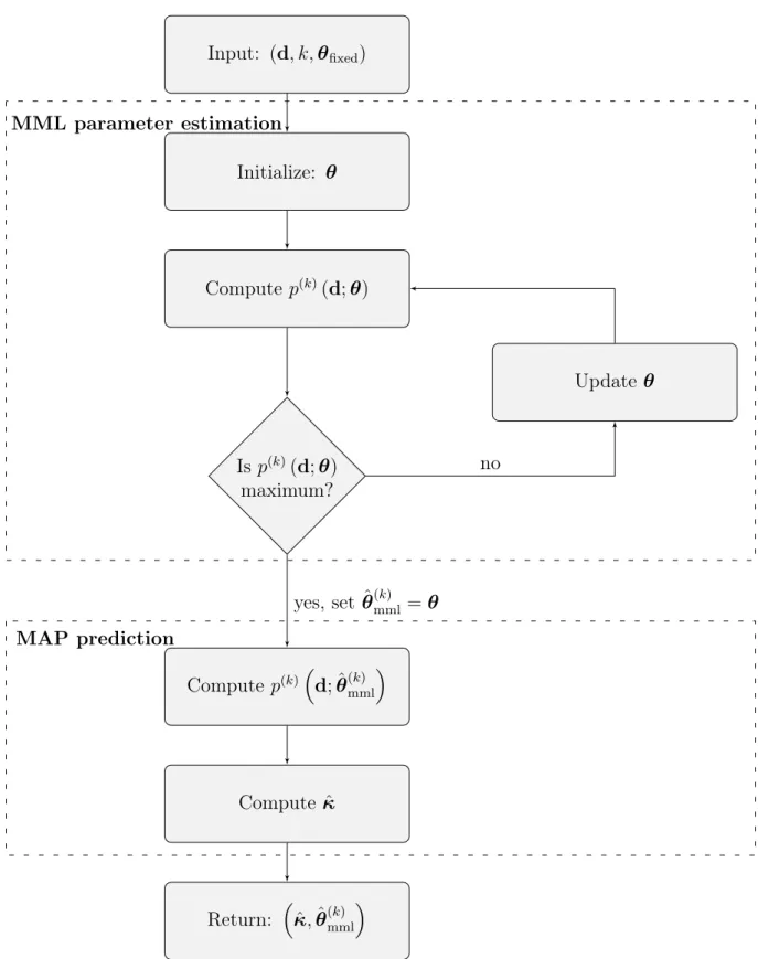
Our workflow is the same as in Lindberg and Omre (2014a), and is given in Fig. 4.1.
We start by initiating the unknown model parameters, θ, and then compute p(k)(d;θ)
using the Forward-Backward algorithm. If the current marginal likelihood is not a
maxi-mum value, we update θ. After convergence, we fix θ(mmlk) equal to the θ that maximizes
p(k)(d;θ). The MAP and MMAP predictors are found based on θˆ(k)
mml.
4.1.2
Approximate Maximum Marginal A Posterior
We present a Bayesian alternative to the approximate MMLE in Section. 4.1.1. A prior
distribution, p(θ), is assigned to the vector of unknown model parameters, θ. The
pos-terior model is then
p(θ|d)∝p(d|θ)p(θ). (4.6)
The mode of Eq. (4.6) is the MAP estimate, θˆ(mapk) . The marginal likelihood, p(d;θ),
is given in Eq. 4.2, but now θ is a random variable. Hence, the posterior p(θ|d) is
proportional to the likelihood, p(d|θ), times the prior of θ. The k-th order approximate
MAP estimate is hence given as
ˆ
θ(mapk) = arg max
θ p(k)(θ|d) = arg max θ logp(k)(d|θ) + logp(θ) = arg max θ logp(θ)−logp(k)(d;θ) (4.7)
Optimization of the approximate marginal likelihood and approximate marginal a poste-rior are therefore similar problems. The approximate maximum MAP estimate should be
evaluated similar as the approximate MMLE. The prior, p(θ), may depend on a set of
hyperparameter, τ = (η,τlr,τla). These could be known, or dependent on another layer
4.1. MARGINAL LIKELIHOOD 31 Input: (d, k,θfixed) Initialize: θ Compute p(k)(d;θ) Is p(k)(d;θ) maximum? Updateθ Compute p(k)d; ˆθ(k) mml Compute κˆ Return: κˆ,θˆ(mmlk) no yes, set ˆθ(mmlk) =θ MML parameter estimation MAP prediction
4.2
The Expectation-Maximization Algorithm
In the following chapter we specify densities dependent on a parameterθ asp(x|θ)instead
of p(x;θ), to clarify the dependence on the parameter. The approximate MML given in
Eq. (4.5), or equivalently the maximum MAP in Eq. (4.7), can be optimized by the expectation-maximization (EM) algorithm. The EM-algorithm was first introduced by Dempster et al. (1977) to overcome difficulties in maximizing likelihoods by introducing latent variables. A thorough introduction to the EM-algorithm is found in Hastie et al. (2001), and Robert and Casella (2005). We present the EM-algorithm in general for a
univariate parameter ν.
We observe x independent and identically distributed from g(x|ν). Assessment of the
maximum likelihood estimator νˆ= arg maxL(ν|x)is often a hard problem. We introduce
an augmented, or latent, variable,z. Let the joint density be denoted byf(x,z|ν). Define
the conditional density of the augmented variable, given the observations, as
h(z|x, ν) = f(x,z|ν)
g(x|ν) . (4.8)
If we rewrite Eq. (4.8) and take the logarithm on both sides, we obtain
logg(x|ν) = logf(x,z|ν)−logh(z|x, ν). (4.9)
We take the expectation on both sides with respect to h(z|x, ν0)for an arbitrary ν0, and
write the conditional densities in terms of log-likelihoods, then,
l(ν|x) = Eν0{l(ν|x,z)} −Eν0{l(z|x,ν)} =Q(ν|ν0)−R(ν0, ν)
. (4.10)
In the E-step we compute Q(ν|ν0,) = Eν0{l(ν|x,z)}, followed by the M-step where
Q(ν|ν0) is maximized with respect to ν. We iterate between the E- and M-step until
convergence. The sequence of estimators {ˆνi}satisfies
l(ˆνi+1|x)≥l(ˆνi|x), (4.11)
with equality if and only if Q(ˆνi+1|ˆνi) = Q(ˆνi|ˆνi). By definition, Q(ˆνi+1|ˆνi)≥Q(ˆνi|νˆi),
since νˆi+1 is defined as the value ν maximizing Q(ν|νˆi). Jensen’s inequality implies
that Eνi log l(z|ˆ νi+1,x) l(z|ˆνi,x) ≤log Eνi p(z| ˆ νi+1,x) p(z|ˆνi,x) = 0. (4.12)
Therefore, we need only to optimize Q(ν|ν0), not R(ν0, ν).
The EM-algorithm provides an increasing sequence of likelihood-values. However, we are
not able to conclude that νˆi converges to the maximum likelihood estimator. In practice
it is necessary to run the EM-algorithm multiple times with different initial values to ensure that the global maximum is found. The EM-algorithm is given in Alg. 3. Cappe et al. (2005) discuss the EM-algorithm and its convergence properties for a hidden Markov model.
In practice the E-step requires calculating the expected log-likelihood, which may consti-tute a hard problem. This can be overcome by estimating the expectation with a Monte Carlo step, see Wei and Tanner (1990). Their method is often referred to as Monte Carlo Expectation Maximization (MCEM).
4.3. MODEL PARAMETERS 33
Algorithm 3: Expectation-Maximization algorithm
Result: Maximum likelihood estimateνˆ
Initialize νˆ0,i= 1
repeat
E-step: Q(ν|ˆνi−1) = Eˆνi−1{l(ν|x,z)}
M-step: νˆi = arg maxνQ(ν|νˆi−1)
i=i+ 1
until convergence;
return νˆ
4.3
Model Parameters
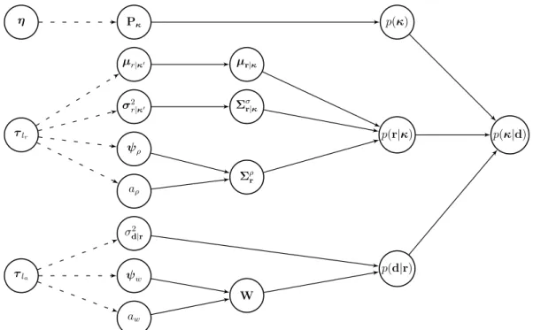
Assessment of the model parameters are in general a hard problem. We present various optimization techniques for the prior, response and acquisition model parameters sepa-rately. We refer to Chapter 3 for an introduction of the model parameters. We assign
independent hyperparameters, η,τlr andτla, to the prior, response and acquisition model
parameters, respectively. In Fig. 4.2 the hierarchical structure of the convolutional model is given. Pκ µr|κ0 σ2 r|κ0 ψρ aρ σ2 d|r ψw aw η τlr τla µr|κ Σσr|κ Σρ r W p(κ) p(r|κ) p(d|r) p(κ|d)
Figure 4.2: Hierarchical structure of the model parameters in the current convolutional model.
4.3.1
Prior Model Parameters
In this section we assume the likelihood model parameters, (θlr,θla), to be known, and
that the only unknown quantity is Pκ, where its dimension is fixed and known. If the