This is the author’s version of a work that was submitted/accepted for pub-lication in the following source:
Denman, Nick, McGree, James, Eccleston, John, & Duffull, Stephen (2011) Design of experiments for bivariate binary responses modelled by Copula functions. Computational Statistics and Data Analysis,55(4), pp. 1509-1520.
This file was downloaded from: http://eprints.qut.edu.au/42929/
Notice: Changes introduced as a result of publishing processes such as copy-editing and formatting may not be reflected in this document. For a definitive version of this work, please refer to the published source:
Design of Experiments for Bivariate Binary Responses Modelled
by Copula Functions
N.G. Denman∗,a, J.M. McGreeb, J.A. Ecclestona, S. B. Duffullc
a
University of Queensland, St. Lucia, Hawken Dr., QLD, 4072 Australia.
b
Queensland University of Technology, GPO Box 2434, Brisbane, QLD, Australia, 4001.
c
University of Otago, Dunedin, Otago, 9001, New Zealand.
Abstract
Optimal design for generalized linear models has primarily focused on univariate data. Often experiments are performed that have multiple dependent responses described by regression type models, and it is of interest and of value to design the experiment for all these responses. This requires a multivariate distribution underlying a pre-chosen model for the data. Here, we consider the design of experiments for bivariate binary data which are dependent. We explore Copula functions which provide a rich and flexible class of structures to derive joint distributions for bivariate binary data. We present methods for deriving optimal experimental designs for dependent bivariate binary data using Copulas, and demonstrate that, by including the dependence between responses in the design process, more efficient parameter estimates are obtained than the usual practice of simply designing for a single variable only. Further, we investigate the robustness of designs with respect to initial parameter estimates and Copula function, and also show the performance of compound criteria within this bivariate binary setting.
Key words: Bivariate binary response, Copulas, Dependence, 𝐷-optimality, Multiple
responses, Multivariate distributions, Optimal design,𝑃-optimality.
1. Introduction
There are many situations where multiple responses are measured during an experi-ment. For example, in pharmacology and in agriculture, parent drug and metabolite concentration, drug toxicity and efficacy, or yield and disease resistance of grain from ∗Corresponding author
Email addresses: [email protected](N.G. Denman),[email protected](J.M. McGree),
a field trial. Poor or incorrect experimental design can lead to inadequate experiments and the subsequent development of models with unsatisfactory properties.
Unlike design of experiments for univariate responses, design for multiple responses has not received much attention. Some early work which considered bivariate binary responses was given by Kanninen (1993) and Alberini (1995). Their focus was on the design of choice experiments where the interest was in estimating as precisely as possible a statistic about the public’s willingness to pay for a change in the environmental quality. However, it is not uncommon for experiments to be designed with respect to a single response variable, ignoring the possibility that more responses might be measured. Design research for multiple response models exists where one response is nested within another, see Waterhouse et al. (2005), Hennig et al. (2007) and McGree et al. (2009). We aim to develop an approach for the design of experiments which yield multiple responses that share a dependence structure.
For dose-ranging trials, Heise and Myers (1996), Dragalin and Fedorov (2006) and Dra-galin et al. (2006) have considered bivariate binary models for the design of experiments where the interest is in the efficacy and toxicity of a drug. Other research in this field has come from Rabie and Flournoy (2004) and Dorta-Guerra et al. (2005). In the context of pharmacokinetic response models, Gueorguieva et al. (2006, 2007), Ogung-benro et al. (2007) have considered optimal design based on the multivariate normal distribution.
We present an approach that is useful when standard multivariate distributions are not applicable (or don’t exist). This approach allows for the specification of arbitrary dependence structures between the responses. Often when designing an experiment, the experimenter knows the distribution of the marginal responses with a high degree of confidence but may not know the joint distribution of the responses. As described by Nelsen (2006), Copulas are distribution functions with uniform marginals that can be used to derive the joint distribution of the multiple responses using the marginal response distributions. This allows arbitrary multivariate distribution functions to be derived that can account for the dependence between the responses. Our work is more general but similar in spirit to Gunduz and Torsney (2006). We concentrate on the bivariate binary response situation but show how this can be extended to a larger class of multivariate data. We conduct an investigation to determine the loss in design efficiency when a dependence structure is not accounted for. We also present a computational exploration into the robustness of optimal designs with respect to initial parameter estimates and Copula functions.
The outline of the paper is as follows. Preliminaries on generalized linear models, design, optimality and the expected Fisher information matrix are given in Section 2. The bivariate binary response model is introduced in Section 3. Copula functions are formally defined and the Fisher information matrix for a general bivariate binary response model is derived. Bivariate binary examples follow in Section 4 where the
robustness of designs and compound criteria are also explored. The paper concludes with a discussion about the key findings and developments in this paper.
2. Preliminaries
2.1. Generalized Linear Model
Each marginal response is assumed to be modelled by a generalized linear model (GLM) as described in McCullagh and Nelder (1989). A GLM is defined by (1) the distribution
of the response, with mean𝝁 =𝐸(𝒀) and variance 𝑉 𝑎𝑟(𝒀) = 𝑎(𝜙)𝑉(𝝁), where 𝑎(𝜙)
is a scale factor that does not depend on𝝁, (2) a linear predictor𝜼=𝑿𝜷 where 𝑿 is
a𝑛×𝑝matrix of covariates and𝜷= (𝛽1, . . . , 𝛽𝑝)′ is a𝑝×1 vector of model parameters
and (3) a link function, 𝑔(𝝅) =𝜼, which links the mean vector to the linear predictor.
We consider binary responses and the expected value of 𝒀 is given by the probability
of success 𝝅. Some common link functions for binary data are the logit link function,
𝑔(𝝅) = logit(𝝅) = log{𝝅/(1−𝝅)}, the probit link function, 𝑔(𝝅) = Φ−1(𝝅), where
Φ(⋅) is the cumulative distribution function of the standard normal distribution and
the complementary log-log link function, 𝑔(𝝅) = log{−log(1−𝝅)}.
2.2. Design
An experimental design𝜉 with 𝑛 support points can be written
𝜉= { 𝒙1 𝒙2 . . . 𝒙𝒏 𝑤1 𝑤2 . . . 𝑤𝑛 } , (1)
where 𝒙𝒊 ∈ 𝒳 are the support points (𝑛-vectors also known as elementary designs)
consisting of the explanatory variables which describe the experimental conditions,
with weights 𝑤𝑖 ∈ [0,1] summing to 1. The design space can be written Ξ ∈ {𝜉 ∈
𝒳 ×[0,1]𝑛:∑𝑛
𝑖=1𝑤𝑖 = 1}. For an exact design with 𝑁 units, the weights are given by
𝑤𝑖 =𝑟𝑖/𝑁 where 𝑟𝑖 is the number of replicates of 𝒙𝒊. For an approximate design, the
weights represent the amount of experimental effort for each support point.
2.3. Fisher Information Matrix
The Fisher information matrix (FIM), 𝑴(𝜽, 𝜉), is the negative expectation of the
second order partial derivatives of the log-likelihood𝑙(𝜽;𝒚) with respect to the model
parameters𝜽. That is,
𝑴(𝜽, 𝜉) = −𝐸 ( ∂2𝑙(𝜽;𝒚) ∂𝜽∂𝜽′ ) . (2)
It is known that the variance-covariance matrix of any unbiased estimator of 𝜽 is
bounded below by𝑴−1(𝜽, 𝜉). Thus, for a given design 𝜉the Fisher information matrix
tells us how well the model parameters are expected to be estimated.
2.4. Optimality
An optimal design is the best choice of design points and corresponding weights with
respect to a given design criterion. A common choice is 𝐷-optimality. A design is
𝐷-optimal if it maximizes the determinant of the Fisher information matrix,∣𝑴(𝜽, 𝜉)∣,
or equivalently, minimizes∣𝑴(𝜽, 𝜉)−1∣. The Cram´er-Rao lower bound given by Cram´er
(1946) says that the optimal design has the minimum variance-covariance for the
max-imum likelihood estimate 𝜽ˆ. Therefore, in general, 𝐷-optimal designs provide good
parameter estimates since they minimize the volume of the joint asymptotic confidence ellipsoid of the parameters.
The 𝐷-efficiency of a design 𝜉 with respect to the optimal design 𝜉∗
𝐷 is given by 𝐷eff = ( ∣𝑴(𝜽, 𝜉)∣ ∣𝑴(𝜽, 𝜉∗ 𝐷)∣ )1/𝑞 , (3)
where𝑞 is the number of model parameters. A𝐷-efficiency of 0.5 means that twice as
much experimental effort is required using𝜉 in order to obtain parameter estimates as
accurate as using𝜉∗
𝐷.
Product𝐷-optimality (see Atkinson and Cox (1974) and Waterhouse et al. (2005)) can
be used to obtain a design with efficient parameter estimates across a number of models. It maximizes the product of the determinants of the Fisher information matrices, scaled by the number of model parameters, for each model.
3. Copulas
There are numerous ways of defining a multivariate distribution for discrete random variables, here we are concerned only with binary responses. Copula functions provide a fruitful source of distribution functions, including those commonly known such as the Archimedian, Clayton, Frank and Gumbel. In the following some background on Copula functions is given, a bivariate binary model defined and the FIM derived.
As described in Sklar (1959), a Copula is a function 𝐶 : [0,1]𝑛→[0,1] that satisfies
1. 𝐶(1, . . . , 𝑢𝑗, . . . ,1) =𝑢𝑗, 𝑗 = 1, . . . , 𝑛 0≤𝑢𝑗 ≤1.
2. 𝐶(𝑢1, . . . , 𝑢𝑛) = 0 if 𝑢𝑗 = 0, 𝑗 = 1, . . . , 𝑛.
Sklar (1959) postulated that there exists a function 𝐶 such that
𝐹(𝑦1, . . . , 𝑦𝑛) = 𝐶(𝐹1(𝑦1), . . . , 𝐹𝑛(𝑦𝑛)). (4)
The converse is if𝐶 is a Copula and𝐹𝑖(𝑦𝑖),𝑖= 1, . . . , 𝑛are marginal distributions then
𝐹(𝑦1, . . . , 𝑦𝑛) is a distribution function. The copula may also be defined as
𝐶(𝑢1, . . . , 𝑢𝑛) =𝐹(𝐹1−1(𝑢1), . . . , 𝐹𝑛−1(𝑢𝑛)). (5)
If all the marginal distributions are continuous, then the Copula is unique. If any of
the marginal distributions are discrete then the Copula is only unique on 𝑅𝑎𝑛(𝐹1)×
⋅ ⋅ ⋅ ×𝑅𝑎𝑛(𝐹𝑛) (see Trivedi and Zimmer (2005) for further details). Since Copulas are
also multivariate distributions then the Fr´echet-Hoeffding lower and upper bounds also apply.
Copula functions allow the specification of multivariate distributions with arbitrary dependence structures. This is a useful tool as distribution functions do not exist for many common situations such as the bivariate binary data case considered here, and more generally for, describing dependence between continuous and discrete data. The next subsection describes some Copula functions for bivariate binary data.
3.1. Bivariate Copulas
A large number of Copulas appear in the literature which impose different dependence relationships between the marginal distribution functions. The books by Hutchinson and Lai (1990), Joe (1997) and Nelsen (2006), and a paper by Trivedi and Zimmer (2005) provide extensive coverage of bivariate Copulas and their properties. In this section, several Copulas that have been used in applications are presented.
An important (and simple) Copula, the product Copula is given by
𝐶(𝑢1, 𝑢2) = 𝑢1𝑢2, 0≤𝑢1, 𝑢2 ≤1. (6) The product Copula corresponds to independence.
3.2. Archimedean Copulas
A bivariate Archimedean Copula (Genest and MacKay (1986)) is defined as
𝐶(𝑢1, 𝑢2;𝛼) =𝜓−1(𝜓(𝑢1;𝛼) +𝜓(𝑢2;𝛼);𝛼) (7)
where𝜓(𝑢), the generator of the Copula, is a class two function with𝜓(1) = 0,𝜓′(𝑢)<0
and𝜓′′(𝑢)>0 for all 0≤𝑢≤1. Archimedean Copulas are commonly used due to their
Clayton Copula
The Clayton Copula (Clayton (1978) and Cook and Johnson (1981)) is given by
𝐶(𝑢1, 𝑢2;𝛼) = ( 𝑢−𝛼 1 +𝑢−2𝛼−1 )−1/𝛼 , 𝛼 >0. (8)
As the dependence parameter 𝛼 → 0, the Clayton Copula approaches (6) and
corre-sponds to independence. As 𝛼 → ∞, the Copula approaches the Fr´echet-Hoeffding
upper bound which is an upper bound on all Copula functions. In the bivariate case, the upper bound represents perfect positive dependence between variates (similarly for
the lower bound and perfect negative dependence). There are no values of𝛼 for which
the Clayton Copula attains the Fr´echet-Hoeffding lower bound. This Copula exhibits strong left tail (with relatively weak right tail) dependence, and cannot account for negative dependence.
Frank Copula
The Frank Copula (Frank (1979)) is given by
𝐶(𝑢1, 𝑢2;𝛼) =−𝛼−1log ( 1 + (𝑒 −𝛼𝑢1 −1) (𝑒−𝛼𝑢2 −1) 𝑒−𝛼−1 ) , 𝛼 ∕= 0 (9)
As the dependence parameter 𝛼 approaches −∞,0,∞, the Copula approaches the
Fr´echet-Hoeffding lower bound, independence and the Fr´echet-Hoeffding upper bound, respectively. This Copula permits negative dependence, and the dependence is sym-metric in both tails. Notably, both Fr´echet-Hoeffding bounds are permissible through
an appropriate choice of 𝛼.
Gumbel Copula
The Gumbel Copula (Gumbel (1960)) is given by
𝐶(𝑢1, 𝑢2;𝛼) = exp
(
−((−log𝑢1)𝛼+ (−log𝑢2)𝛼)1/𝛼
)
, 1≤𝛼 <∞ (10)
As the dependence parameter𝛼 approaches 1 and∞, the Copula approaches
indepen-dence and the Fr´echet-Hoeffding upper bound, respectively. There are no values for𝛼
such that the Copula approaches the Fr´echet-Hoeffding lower bound. This Copula does not allow negative dependence, and exhibits strong right tail (with relatively weak left tail) dependence.
3.3. Bivariate Binary Model
Let (𝑌𝑖1, 𝑌𝑖2),𝑖= 1, . . . , 𝑛be a bivariate binary response. For each observation there are
four possible outcomes{(0,0),(0,1),(1,0),(1,1)}where ‘1’ usually represents a success
and ‘0’ a failure.
For a single observation let
𝑝𝑦1,𝑦2 = Pr (𝑌1 =𝑦1, 𝑌2 =𝑦2), 𝑦1, 𝑦2 = 0,1 (11)
be the joint probabilities of 𝑌1 and 𝑌2. The key is to represent the joint probability of
success using a copula representation as in (4). That is,
𝑝11=𝐶(𝜋1, 𝜋2;𝛼) (12) The remaining joint probabilities can be derived as
𝑝10 = 𝜋1−𝑝11 (13)
𝑝01 = 𝜋2−𝑝11 (14)
𝑝00 = 1−𝜋1−𝜋2+𝑝11, (15)
where𝜋𝑟, 𝑟= 1,2 are the marginal probabilities of success.
Note that the bivariate binary models presented in Dragalin et al. (2006), Dragalin and Fedorov (2006) and Heise and Myers (1996) are special cases of the approach presented above.
The complete log-likelihood for the bivariate binary model can be written
𝑙(𝜽;𝒚) =
𝑛 ∑
𝑖=1
𝑤𝑖𝑙𝑖(𝜽;𝒚), (16)
where 𝜽 = (𝜷1,𝜷2, 𝛼), 𝑤𝑖 are the design weights and the log-likelihood for a single
observation is given by
𝑙𝑖(𝜽;𝒚) = 𝑦1𝑦2log𝑝11+𝑦1(1−𝑦2) log𝑝10+ (1−𝑦1)𝑦2log𝑝01
+ (1−𝑦1)(1−𝑦2) log𝑝00. (17)
The Fisher information for a single observation can be derived as (see also Dragalin and Fedorov (2006)) 𝑴(𝜽, 𝜉𝑖) = ∂𝑝 ∂𝜽 ( 𝑃−1 + 1 1−𝑝11−𝑝10−𝑝01 𝑒𝑒𝑇 ) ∂𝑝 ∂𝜽𝑇 (18)
The expected Fisher information matrix for Copula functions is derived in Appendix A.
4. Applications
In the following examples, designs are derived that allow for efficient estimation of parameters for various dependence structures. Firstly, a hypothetical example is con-sidered to illustrate the methods described earlier. A second example with applications
to pharmacology follows. In both examples, when dependence is assumed, 𝛼 is
pre-sumed to be estimated.
Throughout the examples, a continuous search, simulated annealing algorithm was used to find the optimal designs. This algorithm was based on work given by Corana et al.
(1987) and MATLAB source code can be found atwww.a-grade.info. The algorithm
starts with an initial random design. A burnin of size (say) 500 iterations is used to determine the starting temperature which initializes the annealing process. Designs which yield a larger criterion value are always accepted, while ‘backwards’ steps are taken with certain probabilities to avoid being trapped in local optima. The search continues until a predefined precision has been reached.
4.1. Example 1
Let each marginal response be modelled by a three factor main effects logistic GLM
with initial parameters 𝜷1 = [1,4,1,−1] and 𝜷2 = [1,−0.5,1,−1], with 𝑥𝑗 ∈ [−1,1],
for𝑗 = 1,2,3. That is,
log ( 𝜋1 1−𝜋1 ) = 1 + 4𝑥1+𝑥2−𝑥3, (19) log ( 𝜋2 1−𝜋2 ) = 1−0.5𝑥1+𝑥2−𝑥3. (20)
The dependency between the marginal distributions is modelled using the Frank copula (9).
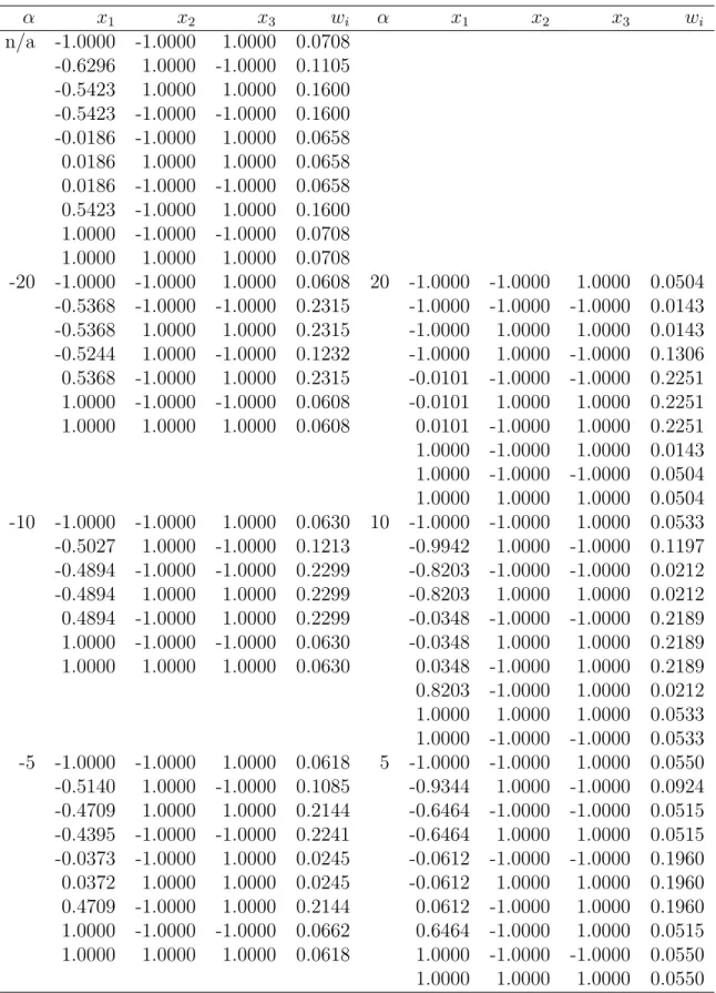
Table 1 shows the 𝐷-optimal designs for the bivariate binary responses described by
equations (19) and (20) and the Frank Copula. The product optimal design (indepen-dent case) is also shown. An initial observation is that assuming a dependence between the two responses can increase the number of support points. In particular, designs for
cases where 𝛼 > 0 can have up to 10 support points. Moreover, some of the optimal
designs shown have less support points than estimable parameters. This is not uncom-mon for multivariate designs, and arises as a consequence of the dependence between
responses. Potentially, each response offers information about any or all parameters from each model. Also, it is possible that the dependence parameter could be ‘free’ to estimate, under some models. This is certainly the case when estimating correlation between two continuous variables, and may extend to this bivariate binary case. Lastly, the designs shown are not necessarily unique in that there may be multiple solutions that maximize the determinant of the Fisher information matrix. This is not uncommon in the univariate case, and may also be seen here in this bivariate situation.
As it may be difficult to determine values of 𝛼 before running the experiment, it is of
interest to know how sensitive or how robust these Copula designs are with respect to
𝛼. Table 2 presents the 𝐷-efficiencies of the designs given in Table 1 with respect to
different 𝛼 values. As expected, the more 𝛼 is misspecified, the greater the reduction
in the 𝐷-efficiencies of the designs. In particular, assuming 𝛼 = −20, when in fact
𝛼= 20, leads to a 𝐷-efficiency of 0.4594 which is a significant loss in terms of efficient
parameter estimation. More interestingly, high𝐷-efficiencies are seen when the sign of
𝛼 is correctly chosen. For example, if it is assumed that 𝛼=−5 when indeed the true
value is 𝛼 =−20, the loss in efficient parameter estimation is minimal shown by a 𝐷
-efficiency of 0.9404. A further observation is that the D-efficiencies are not symmetric
around 𝛼 = 0. That is, assuming 𝛼 = 20, when in fact 𝛼 = −20, does not yield the
same 𝐷-efficiency when assuming 𝛼 = −20, when the true value is 20. This could be
tied into the fact that the joint probabilities are also not symmetric around 𝛼= 0.
When observing bivariate binary responses, it may not be clear if the responses are dependent or not. Hence we explore the loss associated with assuming dependence
when the responses are actually independent. Table 3 shows the 𝐷-efficiencies of the
𝐷-optimal designs for the models describing the bivariate response in the dependent and
independent cases with respect to the two univariate response models (equations (19)
and (20)). The design which yields the highest product of the two 𝐷-efficiencies is the
product𝐷-optimal design as this is (essentially) what is maximized to find this design.
Importantly, the results show that little is lost (with respect to the product design)
when a dependence is assumed between the two bivariate responses. In fact, similar𝐷
-efficiencies are seen for all designs. This means that assuming some dependence between the responses does not drastically compromise parameter estimation if the responses are in fact independent.
As mentioned earler, it is common to design such studies by assuming the two responses are independent. In order to determine how much is lost by assuming independence, when in fact a dependence structure exists, the product design was compared with the
𝐷-optimal Copula designs. Table 4 shows the performance of the product 𝐷-optimal
design in estimating parameters (including 𝛼) when a dependence exists between the
two responses. When 𝛼 < 10, the 𝐷-efficiencies are quite reasonable suggesting the
product𝐷-optimal design would perform quite well at estimating the model parameters
and 𝛼. However, when 𝛼 = 20, the 𝐷-efficiency becomes quite reduced. This shows
0 2 4 6 8 10 0 0.2 0.4 0.6 0.8 1 α = −20 Dose Probability 0 2 4 6 8 10 0 0.2 0.4 0.6 0.8 1 α = −10 Dose Probability 0 2 4 6 8 10 0 0.2 0.4 0.6 0.8 1 α = −5 Dose Probability 0 2 4 6 8 10 0 0.2 0.4 0.6 0.8 1 α = 5 Dose Probability 0 2 4 6 8 10 0 0.2 0.4 0.6 0.8 1 α = 10 Dose Probability 0 2 4 6 8 10 0 0.2 0.4 0.6 0.8 1 Dose Probability α = 20
Efficacy and toxicity (p11) Efficacy without toxicity (p10) Toxicity without efficacy (p01) No efficacy, no toxicity (p00)
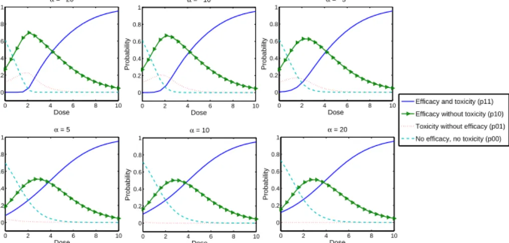
Figure 1: Probabilities 𝑝11, 𝑝10, 𝑝01 and 𝑝00 given by models (21), Frank Copula and 𝛼 =
−20,−10,−5,5,10 and 20.
compromise parameter estimation.
4.2. Example 2
Consider a clinical trial where the responses are efficacy and toxicity. Let 𝑌1
repre-sent efficacy and 𝑌2 toxicity. We denote the joint probabilities by (12) with marginal
probabilities of success given by log ( 𝜋𝑖 1−𝜋𝑖 ) =𝛽𝑖0+𝛽𝑖1𝑑 𝑖= 1,2 (21)
where𝑑∈[0,10] represents dose and initial parameters 𝜷1 = [−1,1] and𝜷2 = [−2,0.5]
are taken from Heise and Myers (1996) and the Frank copula is given by (9).
Figure 1 shows the joint probabilities 𝑝11, 𝑝10, 𝑝01 and 𝑝00 for various values of 𝛼 as
a function of dose. The probability of achieving efficacy and toxicity (𝑝11) increases
with dose with the opposite being true for𝑝00; the probability of not achieving efficacy
and no toxicity. The probability of achieving efficacy without toxicity (𝑝10) initially
increases with dose until dose becomes too ‘large’. At this point 𝑝10 decreases as the
toxic effect of the drug becomes more likely. Finally, the probability of toxicity without
efficacy 𝑝01 is generally quite small (<0.2).
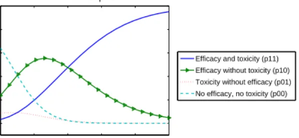
As a comparison to Figure 1, Figure 2 shows the joint probabilities where the two binary
responses are independent. Hence, the product copula was used to calculate 𝑝11, 𝑝10,
𝑝01 and 𝑝00 for 𝑑 ∈ [0,10]. Differences between the joint probabilities are particularly
0 2 4 6 8 10 0 0.2 0.4 0.6 0.8 1 Dose Probability Product Copula
Efficacy and toxicity (p11) Efficacy without toxicity (p10) Toxicity without efficacy (p01) No efficacy, no toxicity (p00)
Figure 2: Probabilities𝑝11,𝑝10, 𝑝01 and𝑝00 given by models (21) and the Product Copula.
shows that the joint probabilities are not symmetric around𝛼 = 0.
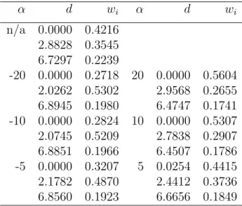
Table 5 show the𝐷-optimal designs for the independent and dependent responses
de-scribed by equation (21). All designs have three similar support points. In comparison with the first example, assuming a dependence between the responses does not increase
the number of support points. Further the similarity of all 𝐷-optimal designs suggest
that, in this case, the designs are robust to variation in 𝛼.
The previous example explored the robustness of 𝐷-optimal designs when 𝛼 was
mis-specified. For this example, a simulation study was run to determine if such designs
were robust to all model parameters (𝜷1, 𝜷2 and 𝛼) for 𝛼 equaling -20, -10, -5, 5, 10
and 20. The study was run by assigning each parameter an upper and lower bound.
These bounds were arbitrary chosen as the initial parameters±1 (respectively). Model
parameters were randomly and uniformly drawn from these intervals and the𝐷-optimal
design constructed. The 𝐷-efficiency of this design compared to those given in Table
5 was then calculated. This was repeated 250 times and the results are summarized in Table 6.
From Table 6, all (mean)𝐷-efficiencies are reasonable for𝛼 >−20 given the uncertainty
assumed around the initial parameter estimates. This shows that such designs will still be able to efficiently estimate misspecified model parameters. Such a property
is important in nonlinear design situations as a 𝐷-optimal design is dependent upon
the initial model parameters specified. For 𝛼 = −20, the misspecification of initial
estimates does seem to affect parameter estimation. In such cases, it may be advisable to explore techniques to provide some robustness properties to this design.
4.2.1. Compound Criteria
We further explore optimal design for the description of the efficacy and toxicity of a drug. In phase I/II trials, it is desirable to administer doses such that model parameters can be estimated as well as possible and also maximize the probability of efficacy
without toxicity. This requires the derivation of designs to address dual goals of an experiment. Compound optimal design crtieria construct designs for this purpose. Such criteria have a long history, see Lauter (1974), Lauter (1976), Lee (1987), Lee (1988), Cook and Wong (1994), Clyde and Chaloner (1994), Huang and Wong (1998), Wong (1999) and McGree et al. (2008).
We focus on combining 𝐷-optimality with a form of 𝑃-optimality (as proposed in
McGree and Eccleston (2008)). 𝑃-optimality aims at maximizing the probability of
certain outcomes. Such designs in this context will place all experimental effort on the (single) dose that maximizes the joint probability of efficacy without toxicity. These objective functions are combined by jointly maximizing a weighted linear combination of the logarithm of each criterion (see Atkinson (2008) and McGree and Eccleston (2008)). The weighting is predefined and allows the experimenter to place more or less emphasis on estimation or maximizing certain probabilities. We will only consider the equally
weighted scenario. Designs found under such a criterion will be termed𝐷𝑃-optimal.
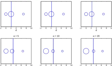
Figure 3 presents the𝐷- and𝑃-optimal designs for the dependent responses described
by equation (21) for 𝛼 = −20,−10,−5,5,10 and 20. The circles represent the 𝐷
-optimal designs with the dose shown by the location and weight shown by the area of
the circles. Since 𝑃-optimal designs only consist of a single support point, they are
represented by the straight vertical line. Notably, the plots suggest that the𝐷-optimal
design for 𝛼 =−20 will be relatively 𝑃-efficient as much of the experimental effort is
placed approximately on the P-optimal support point. This is in contrast to 𝛼 = 20,
where only a small circle is seen about the 𝑃-optimal design.
−2 0 2 4 6 8 10 d α = −20 −2 0 2 4 6 8 10 d α = −10 −2 0 2 4 6 8 10 d α = −5 −2 0 2 4 6 8 10 d α = 5 −2 0 2 4 6 8 10 d α = 10 −2 0 2 4 6 8 10 d α = 20
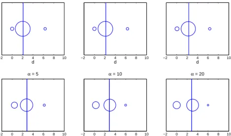
Figure 4 shows the𝐷𝑃-optimal designs when each criterion is equally weighted. That
is, both estimation and maximizing 𝑝10 are believed to be of equal importance. In
comparison to Figure 3, the shift in experimental effort around the 𝑃-optimal design
is obvious. Such designs are therefore more likely to produce efficacious and non-toxic responses. The trade-off is that parameter estimation will be compromised. Table
7 shows the 𝐷-efficiencies of the 𝐷𝑃-optimal designs. All efficiencies are quite high
suggesting that the compromise in estimation is minimal.
−2 0 2 4 6 8 10 d α = −20 −2 0 2 4 6 8 10 d α = −10 −2 0 2 4 6 8 10 d α = −5 −2 0 2 4 6 8 10 d α = 5 −2 0 2 4 6 8 10 d α = 10 −2 0 2 4 6 8 10 d α = 20
Figure 4: 𝐷𝑃-optimal designs with each criterion is equally weighted and𝛼=−20,−10,−5,5,10 and 20.
4.2.2. Different Copula Function?
One obvious design question is, how robust are 𝐷-optimal designs with respect to
the choice of Copula? This is a difficult question to answer as an 𝛼 value for one
Copula will have a different meaning and indeed induce a different dependence between
responses within another Copula. With this in mind, 𝐷-efficiencies of optimal designs
were compared under different Copulas with the parameter estimates held fixed. That
is, the 𝐷-optimal design under (for example) the Frank Copula with a certain set of
parameters was derived. The performance of this design was then compared with the
𝐷-optimal designs under the Clayton and Gumbel Copula functions (with the same
set of initial parameter estimates used in the Frank Copula). The𝐷-efficiencies of this
comparison will then suggest how robust designs are with respect to different Copula
functions. Table 8 presents these𝐷-efficiencies. All are high meaning that, even though
different dependence structures were assumed between the two responses, relatively similar designs were found. This may be a consequence of the very limited information
content within binary data. That is, the subtle differences in dependence structures may be difficult to see when the responses are binary. Further, it does suggest that, for this example, the Copula function (and therefore the dependence structure) is not overly important when designing this experiment. This is useful information as little is lost in terms of parameter estimation if different Copula functions are used to model the data.
5. Conclusion
There are many situations where multivariate data (in particular bivariate data) are observed from an experiment. This paper has developed an approach and methodology for optimally designing such experiments for bivariate binary data. The innovative use of Copulas permits a wide class of possible models to be considered. It has been demonstrated that through our results the dependence between bivariate data can be utilized to derive a more efficient experiment. Two specific examples were considered. A generic GLM example and an application to toxicity/efficacy trials. These examples showed the gains in efficiency and improvement in precision of the parameter estimates for each response when the dependence is acknowledged. While our work provides the impetus for consideration of multivariate methods across the spectrum of response variable types that might be seen in toxicity/efficacy trials, it should not necessarily be limited to this particular application, and is indeed more generally applicable to multivariate data. Pharmacology trials should be analyzed in the same manner in which they are designed such that a Copula method would be required in analysis to ensure the benefits of the optimal design.
Robustness investigations were also undertaken. Initially it was found that when the correct sign of the dependence parameter was assumed for the Frank Copula, all designs
were highly 𝐷-efficient, despite variation in 𝛼. When significant uncertainty exists in
the initial parameter estimates, the precision of estimates was compromised in some cases. Therefore, it is advisable to consider implementing compromise techniques as a means of guarding against such pitfalls. Further, for the example considered, the choice of Copula seemed inconsequential in terms of estimation. Therefore, it may be that simply assuming a dependence (with the right sign) modelled by some Copula is enough to derive a robust, efficient experimental design. This needs requires further investigation.
These methods can be generalized to different multivariate situations with the accom-panying increased degree of complexity dependent on the dimension of the situation. Similar approaches to those used here are being developed for other discrete random variables, the Poisson being the most obvious, and the situation where one response is discrete and the other continuous, such as a binary and a normal making up the bivariate responses.
Acknowledgement
We would like to thank Sue Lewis and Dave Woods from the University of Southampton and Ken Russell from the University of Wollongong for their helpful discussions.
References
Alberini, A., 1995. Optimal designs for discrete choice contingent valuation surveys: Single bounded, double bounded and bivariate models. Journal of Environmental Economics and Management 28, 287–306.
Atkinson, A., 2008. DT-optimum designs for model discrimination and parameter esti-mation. Journal of Statistical Planning and Inference 138, 56–64.
Atkinson, A. C., Cox, D., 1974. Planning experiments for discriminating between mod-els. Journal of the Royal Statistical Society, Series B (Methodological) 36, 321–348. Clayton, D. G., 1978. A model for association in bivariate life tables and its
appli-cation in epidemiological studies for familial tendency in chronic disease incidence. Biometrika 65, 141–151.
Clyde, M., Chaloner, K., 1994. The equivalence of constrained and weighted designs in multiple objective design problems. Journal of the American Statistical Association 91, 1236–1244.
Cook, R. D., Johnson, M. E., 1981. A family of distributions for modelling non-elliptically symmetric multivariate data. Journal of the Royal Statistical Society, Series B (Methodological) 43, 210–218.
Cook, R. D., Wong, W. K., 1994. On the equivalence of constrained and compound optimal designs. Journal of the American Statistical Association 89, 687–692.
Corana, A., Marchesi, M., Martini, C., Ridella, S., 1987. Minimizing multimodal func-tions of continuous variables with the ‘simulated annealing’ algorithm. ACM Trans-actions on Mathematical Software 13, 262–280.
Cram´er, H., 1946. Mathematical methods of statistics. Princeton, NJ: Princeton Uni-versity Press, 474–477.
Dorta-Guerra, R., Gonzalez-Davina, E., Ginebra, J., 2005. Two-level experiments for binary response data, Universidad Politecnica de Cataluna, Barcelona.
Dragalin, V., Fedorov, V., 2006. Adaptive designs for dose-finding based on efficacy-toxicity response. Journal of Statistical Planning and Inference 136, 1800–1823.
Dragalin, V., Fedorov, V., Wu, Y., 2006. Optimal designs for bivariate probit model, technical Report 2006-01, GKS.
Frank, M. J., 1979. On the simultaneous associativity of f(x; y) and x + y - f(x; y). Aequationes Math 19, 194–226.
Genest, C., MacKay, J., 1986. The joy of copulas: Bivariate distributions with uniform marginals. The American Statistician 40, 280–283.
Gueorguieva, I., Aarons, L., Ogungbenro, K., Jorga, K. M., Rodgers, T., Rowland, M., 2006. Optimal design for multivariate response pharmacokinetic models. The Journal of Pharmacokinetics and Pharmacodynamics 33, 97–124.
Gueorguieva, I., Ogungbenro, K., Graham, G., Glatt, S., Aarons, L., 2007. A pro-gram for individual and population optimal design for univariate and multivariate response pharmacokinetic-pharmacodynamic models. Computer Methods and Pro-grams in Biomedicine 86, 51–61.
Gumbel, E. J., 1960. Distributions des valeurs extremes en plusieurs dimensions. Pub-lications de l’Institute de Statist´ıque de l’Universit´e de Paris 9, 171–173.
Gunduz, N., Torsney, B., 2006. Some advances in optimal designs in contingent valua-tion studies. Journal of Statistical Planning and Inference 136, 1153–1165.
Heise, M. A., Myers, R. H., 1996. Optimal designs for bivariate logistic regression. Biometrics 52, 613–624.
Hennig, S., Waterhouse, T. H., Bell, S. C., France, M., Wainwright, C. E., Miller, H., Charles, B. G., Duffull, S. B., 2007. A D-optimal designed population pharmacoki-netic study of oral itraconazole in adult cystic fibrosis patients. British Journal of Clinical Pharmacology 63, 438–450.
Huang, Y. C., Wong, W. K., 1998. Multiple-objective optimal designs. Journal of Bio-pharmaceutical Statistics 8, 635–643.
Hutchinson, T. P., Lai, C. D., 1990. Continuous Bivariate Distributions, Emphasising Applications. Rumsby, Sydney, Australia.
Joe, H., 1997. Multivariate Models and Dependence Concepts. Chapman and Hall, London.
Kanninen, B. J., 1993. Optimal experimental design for double-blinded dichotomous choice contingent valuation. Land Economics 69, 138–146.
Lauter, E., 1974. Experimental planning in a class of models. Mathematishe Opera-tionsforschung und Statisik 5, 673–708.
Lauter, E., 1976. Optimal multipurpose designs for regression models. Mathematishe Operationsforschung und Statisik 7, 51–68.
Lee, C. M. S., 1987. Constrained optimal designs for regression models. Communications in Statistics, Part A - Theory and Models 16, 765–783.
Lee, C. M. S., 1988. Constrained optimal design. Journal of Statistical Planning and Inference 18, 377–389.
McCullagh, P., Nelder, J. A., 1989. Generalized Linear Models, 2nd Edition. Chapman and Hall.
McGree, J. M., Duffull, S. B., Eccleston, J. A., 2008. Compound optimal design criteria for nonlinear models. Journal of Biopharmaceutical Statistics 18, 646–661.
McGree, J. M., Eccleston, J. A., 2008. Probability-based optimal design. Australian and New Zealand Journal of Statistics 50, 1–16.
McGree, J. M., Eccleston, J. A., Duffull, S. B., 2009. Simultaneous vs. sequential design for nested multiple response models with FO and FOCE considerations. Journal of Pharmacokinetics and Pharmacodynamics 36, 101–123.
Nelsen, R. B., 2006. An Introduction to Copulas, 2nd Edition. Springer, New York. Ogungbenro, K., Gueorguieva, I., Majid, O., Graham, G., Aarons, L., 2007. Optimal
design for multiresponse pharmacokinetic models - dealing with unbalanced designs. Journal of Pharmacokinetics and Pharmacodynamics 34, 313–331.
Rabie, H. S., Flournoy, N., 2004. Optimal designs for the contingent response model. In mODa 7 - Advances in Model-Oriented Design and Analysis, Di Bucchianico, A., Lauter, H. and Wynn, H. P. (Eds) Physica-Verlag, 133–142.
Sklar, A., 1959. Fonctions de repartition ´a𝑛 dimensions et leurs marges. Publications
de l’Institute de Statist´ıque de l’Universit´e de Paris 8, 229–231.
Trivedi, P. K., Zimmer, D. M., 2005. Copula modeling: An introduction for practition-ers. Econometrics 1, 1–111.
Waterhouse, T. H., Redmann, S., Duffull, S. B., Eccleston, J. A., 2005. Optimal de-sign for model discrimination and parameter estimation for itraconazole popu- lation pharmacokinetics in cystic fibrosis patients. Journal of Pharmacokinetics and Phar-macodynamics 32, 521–545.
Wong, W. K., 1999. Multiple-objective optimal designs. Recent advances in multiple-objective design strategies 53, 257–276.
A. Derivation of the expected Fisher information matrix
To derive𝑴(𝜽, 𝜉) for Copula functions, we need the following derivatives.
∂𝑝11 ∂𝜷𝒊 = ∂𝐶 ∂𝜋𝑖 ∂𝜋𝑖 ∂𝜷𝒊 , 𝑖= 1,2 (22) ∂𝑝10 ∂𝜷1 = ( 1− ∂𝐶 ∂𝜋1 ) ∂𝜋1 ∂𝜷1 (23) ∂𝑝10 ∂𝜷2 = − ∂𝐶 ∂𝜋2 ∂𝜋2 ∂𝜷2 (24) ∂𝑝01 ∂𝜷1 = − ∂𝐶 ∂𝜋1 ∂𝜋1 ∂𝜷1 (25) ∂𝑝01 ∂𝜷2 = ( 1− ∂𝐶 ∂𝜋2 ) ∂𝜋2 ∂𝜷2 (26) ∂𝑝11 ∂𝛼 = − ∂𝑝10 ∂𝛼 =− ∂𝑝01 ∂𝛼 = ∂𝐶 ∂𝛼 (27)
Thus𝑴(𝜽, 𝜉) can be written
𝑴(𝜽, 𝜉) = 𝑱 ( 𝑷−1+ 1 1−𝑝11−𝑝10−𝑝01 𝒆𝒆𝑇 ) 𝑱𝑇 (28) where 𝑱 = ( 𝑱1𝑱2 ∂𝐶 ∂𝛼 − ∂𝐶 ∂𝛼 − ∂𝐶 ∂𝛼 ) (29) and 𝑱1 = ( ∂𝜋1 ∂𝜷1 0 0 ∂𝜋2 ∂𝜷2 ) , 𝑱2 = ( ∂𝐶 ∂𝜋1 1− ∂𝐶 ∂𝜋1 − ∂𝐶 ∂𝜋1 ∂𝐶 ∂𝜋2 − ∂𝐶 ∂𝜋2 1− ∂𝐶 ∂𝜋2 ) (30)
Considering the product copula (6), the Fisher information matrix can be derived as
𝑀(𝜃, 𝜉) = 𝑛 ∑ 𝑖=1 𝑱1𝑱2𝑽 𝑱2𝑇𝑱1𝑇 (31) = 𝑛 ∑ 𝑖=1 𝑱1 ( 1 𝜋1(1−𝜋1) 0 0 1 𝜋2(1−𝜋2) ) 𝑱1𝑇, (32) where 𝑱2 = ( 𝜋2 1−𝜋2 −𝜋2 𝜋1 1−𝜋1 −𝜋1 ) . (33)
It can be seen that maximizing the determinant of (32) is equivalent to maximizing the product of the determinants of the individual information matrices for each response.
Table 1: 𝐷-optimal product and copula designs for𝛼=−20,−10,−5,5,10 and 20. 𝛼 𝑥1 𝑥2 𝑥3 𝑤𝑖 𝛼 𝑥1 𝑥2 𝑥3 𝑤𝑖 n/a -1.0000 -1.0000 1.0000 0.0708 -0.6296 1.0000 -1.0000 0.1105 -0.5423 1.0000 1.0000 0.1600 -0.5423 -1.0000 -1.0000 0.1600 -0.0186 -1.0000 1.0000 0.0658 0.0186 1.0000 1.0000 0.0658 0.0186 -1.0000 -1.0000 0.0658 0.5423 -1.0000 1.0000 0.1600 1.0000 -1.0000 -1.0000 0.0708 1.0000 1.0000 1.0000 0.0708 -20 -1.0000 -1.0000 1.0000 0.0608 20 -1.0000 -1.0000 1.0000 0.0504 -0.5368 -1.0000 -1.0000 0.2315 -1.0000 -1.0000 -1.0000 0.0143 -0.5368 1.0000 1.0000 0.2315 -1.0000 1.0000 1.0000 0.0143 -0.5244 1.0000 -1.0000 0.1232 -1.0000 1.0000 -1.0000 0.1306 0.5368 -1.0000 1.0000 0.2315 -0.0101 -1.0000 -1.0000 0.2251 1.0000 -1.0000 -1.0000 0.0608 -0.0101 1.0000 1.0000 0.2251 1.0000 1.0000 1.0000 0.0608 0.0101 -1.0000 1.0000 0.2251 1.0000 -1.0000 1.0000 0.0143 1.0000 -1.0000 -1.0000 0.0504 1.0000 1.0000 1.0000 0.0504 -10 -1.0000 -1.0000 1.0000 0.0630 10 -1.0000 -1.0000 1.0000 0.0533 -0.5027 1.0000 -1.0000 0.1213 -0.9942 1.0000 -1.0000 0.1197 -0.4894 -1.0000 -1.0000 0.2299 -0.8203 -1.0000 -1.0000 0.0212 -0.4894 1.0000 1.0000 0.2299 -0.8203 1.0000 1.0000 0.0212 0.4894 -1.0000 1.0000 0.2299 -0.0348 -1.0000 -1.0000 0.2189 1.0000 -1.0000 -1.0000 0.0630 -0.0348 1.0000 1.0000 0.2189 1.0000 1.0000 1.0000 0.0630 0.0348 -1.0000 1.0000 0.2189 0.8203 -1.0000 1.0000 0.0212 1.0000 1.0000 1.0000 0.0533 1.0000 -1.0000 -1.0000 0.0533 -5 -1.0000 -1.0000 1.0000 0.0618 5 -1.0000 -1.0000 1.0000 0.0550 -0.5140 1.0000 -1.0000 0.1085 -0.9344 1.0000 -1.0000 0.0924 -0.4709 1.0000 1.0000 0.2144 -0.6464 -1.0000 -1.0000 0.0515 -0.4395 -1.0000 -1.0000 0.2241 -0.6464 1.0000 1.0000 0.0515 -0.0373 -1.0000 1.0000 0.0245 -0.0612 -1.0000 -1.0000 0.1960 0.0372 1.0000 1.0000 0.0245 -0.0612 1.0000 1.0000 0.1960 0.4709 -1.0000 1.0000 0.2144 0.0612 -1.0000 1.0000 0.1960 1.0000 -1.0000 -1.0000 0.0662 0.6464 -1.0000 1.0000 0.0515 1.0000 1.0000 1.0000 0.0618 1.0000 -1.0000 -1.0000 0.0550 1.0000 1.0000 1.0000 0.0550
Table 2: 𝐷-efficiencies as a measure of the robustness of the𝐷-optimal designs with respect to𝛼being misspecified. Assumed 𝛼 -20 -10 -5 5 10 20 -20 1.0000 0.9800 0.9404 0.7006 0.5631 0.5106 -10 0.9917 1.0000 0.9919 0.8389 0.7727 0.7453 True𝛼 -5 0.9852 0.9971 1.0000 0.9522 0.9222 0.9068 5 0.8928 0.9139 0.9358 1.0000 0.9949 0.9884 10 0.7071 0.7340 0.7842 0.9905 1.0000 0.9969 20 0.4594 0.4783 0.5975 0.9503 0.9904 1.0000
Table 3: 𝐷-efficiencies of designs for models assuming independent and dependent data (Table 1) with respect to univariate response models.
Model 𝛼= -20 𝛼= -10 𝛼= -5 𝛼 = 5 𝛼= 10 𝛼= 20 Prod.
1 0.8287 0.8293 0.8250 0.8376 0.8437 0.8479 0.8216
2 0.7338 0.7349 0.7365 0.7056 0.6850 0.6744 0.7602
1×2 0.6081 0.6095 0.6076 0.5910 0.5779 0.5718 0.6246
Table 4: 𝐷-efficiencies of the product design (Table 1 with𝛼= n/a) with respect to𝐷-optimal copula designs (Table 1 with𝛼=−20,−10,−5,5,10 and 20).
𝛼 -20 -10 -5 5 10 20
Table 5: 𝐷-optimal designs for independent and dependent responses where models for both responses are given by equation (21) and the Frank Copula is assumed for the dependent responses.
𝛼 𝑑 𝑤𝑖 𝛼 𝑑 𝑤𝑖 n/a 0.0000 0.4216 2.8828 0.3545 6.7297 0.2239 -20 0.0000 0.2718 20 0.0000 0.5604 2.0262 0.5302 2.9568 0.2655 6.8945 0.1980 6.4747 0.1741 -10 0.0000 0.2824 10 0.0000 0.5307 2.0745 0.5209 2.7838 0.2907 6.8851 0.1966 6.4507 0.1786 -5 0.0000 0.3207 5 0.0254 0.4415 2.1782 0.4870 2.4412 0.3736 6.8560 0.1923 6.6656 0.1849
Table 6: Mean 𝐷-efficiencies (over 250 random sets of model parameters) of the 𝐷-optimal copula designs for𝛼=−20,−10,−5,5,10 and 20.
𝛼 -20 -10 -5 5 10 20
Mean D-efficiency 0.5595 0.7391 0.8119 0.8222 0.8202 0.7654
Table 7: 𝐷-efficiencies for the𝐷𝑃-optimal designs for𝛼=−20,−10,−5,5,10 and 20.
𝛼 -20 -10 -5 5 10 20
Table 8: 𝐷-efficiencies of𝐷-optimal designs with respect to the Clayton, Frank and Gumbel Copulas with𝛼= 1,5,10,15 and 20.
True Copula Assumed Copula 𝛼 = 1 𝛼= 5 𝛼= 10 𝛼= 15 𝛼= 20
Clayton Frank 0.9866 0.9786 0.8738 0.8566 0.8381 Gumbel 0.9664 0.9786 0.8667 0.8475 0.8342 Frank Clayton 0.9866 0.9811 0.9153 0.8867 0.8767 Gumbel 0.9776 0.9789 0.9978 0.9998 0.9999 Gumbel Clayton 0.9695 0.9727 0.9005 0.8764 0.8708 Frank 0.9815 0.9658 0.9972 0.9998 0.9999