Deep Canonical Time Warping
for simultaneous alignment and representation
learning of sequences
George Trigeorgis, Mihalis A. Nicolaou,
Member, IEEE,
Bj ¨orn W. Schuller,
Senior member, IEEE
Stefanos Zafeiriou,
Member, IEEE
Abstract—Machine learning algorithms for the analysis of time-series often depend on the assumption that utilised data are temporally aligned. Any temporal discrepancies arising in the data is certain to lead to ill-generalisable models, which in turn fail to correctly capture properties of the task at hand. The temporal alignment of time-series is thus a crucial challenge manifesting in a multitude of applications. Nevertheless, the vast majority of algorithms oriented towards temporal alignment are either applied directly on the observation space or simply utilise linear projections - thus failing to capture complex, hierarchical non-linear representations that may prove beneficial, especially when dealing with multi-modal data (e.g., visual and acoustic information). To this end, we present Deep Canonical Time Warping (DCTW), a method that automatically learns non-linear representations of multiple time-series that are (i) maximally correlated in a shared subspace, and (ii) temporally aligned. Furthermore, we extend DCTW to a supervised setting, where during training, available labels can be utilised towards enhancing the alignment process. By means of experiments on four datasets, we show that the representations learnt significantly outperform state-of-the-art methods in temporal alignment, elegantly handling scenarios with heterogeneous feature sets, such as the temporal alignment of acoustic and visual information.
Index Terms—time warping, cca, lda, dcca, dda, deep learning, shared representations, dctw
F
1
I
NTRODUCTIONT
HE alignment of multiple data sequences is a com-monly arising problem, raised in multiple fields related to machine learning, such as signal, speech and audio analysis [33], computer vision [6], graphics [5] and bio-informatics [1]. Example applications range from the tem-poral alignment of facial expressions and motion capture data [43], [44], to the alignment for human action recogni-tion [40], and speech [22].The most prominent temporal alignment method is Dynamic Time Warping (DTW) [33], which identifies the optimal warping path that minimises the Euclidean distance between two time-series. While DTW has found wide application over the past decades, the application is limited mainly due to the inherent inability of DTW to handle observations of different or high dimensionality since it di-rectly operates on the observation space. Motivated by this limitation while recognising that this scenario is commonly encountered in real-world applications (e.g., capturing data from multiple sensors), in [43] an extension to DTW is proposed. Coined Canonical Time Warping (CTW), the method combines Canonical Correlation Analysis (CCA) and DTW by aligning the two sequences in a common, latent subspace of reduced dimensionality whereon the • G. Trigeorgis, S. Zafeiriou, and B. W. Schuller are with the Department of
Computing, Imperial College London, SW7 2RH, London, UK E-mail: [email protected]
• Mihalis A. Nicolaou is with the Department of Computing at Goldsmiths, University of London
E-mail: [email protected]
• Stefanos Zafeiriou is also with Center for Machine Vision and Signal Analysis, University of Oulu, Finland.
two sequences are maximally correlated. Other extensions of DTW include the integration of manifold learning, thus facilitating the alignment of sequences lying on different manifolds [15], [40] while in [36], [44] constraints are intro-duced in order to guarantee monotonicity and adaptively constrain the temporal warping. It should be noted that in [44], a multi-set variant of CCA is utilised [18] thus enabling the temporal alignment of multiple sequences, while a Gauss-Newton temporal warping method is proposed.
While methods aimed at solving the problem of tempo-ral alignment have been successful in a wide spectrum of applications, most of the aforementioned techniques find a single linear projection for each sequence. While this may suffice for certain problem classes, in many real world applications the data are likely to be embedded with more complex, possibly hierarchical and non-linear structures. A prominent example lies in the alignment of non-linear acoustic features with raw pixels extracted from a video stream (for instance, in the audiovisual analysis of speech, where the temporal misalignment is a common problem). The mapping between these modalities is deemed highly nonlinear, and in order to appropriately align them in time this needs to be taken into account. An approach towards extracting such complex non-linear transformations is via adopting the principles associated with the recent revival of deep neural network architectural models. Such archi-tectures have been successfully applied in a multitude of problems, including feature extraction and dimensionality reduction [20], feature extraction for object recognition and detection [14], [25], feature extraction for face recognition [37], acoustic modelling in speech recognition [19], as well
as for extracting non-linear correlated features [2].
Of interest to us is also work that has evolved around multimodal learning. Specifically, deep architectures deemed very promising in several areas, often overcoming by a large margin traditionally used methods in various emotion and speech recognition tasks [24], [29], and on robotics applications with visual and depth data [41].
In this light, we propose Deep Canonical Time Warping (DCTW), a novel method aimed towards the alignment of multiple sequences that discovers complex, hierarchical representations which are both maximally correlated and
temporally aligned. To the best of our knowledge, this work presents thefirst deep approach towards solving the prob-lem of temporal alignment1, which in addition offers very good scaling when dealing with large amounts of data. In more detail, this paper carries the following contributions: (i) we extend DTW-based temporal alignment methods to handle heterogeneous collections of features that may be connected via non-linear hierarchical mappings, (ii) in the process, we extend DCCA to (a) handle arbitrary temporal discrepancies in the observations and (b) cope with multiple (more than two) sequences, while (iii) we extend DCCA and DCTW in order to extract hierarchical, non-linear fea-tures in the presence of labelled data, thus enriched with
discriminativeproperties. In order to do so, we exploit the optimisation problem of DCCA in order to provide a deep counterpart of Linear Discriminant Analysis (LDA), that is subsequently extend with time-warpings. We evaluate the proposed methods on a multitude of real data sets, where the performance gain in contrast to other state-of-the-art methods becomes clear.
The remainder of this paper is organised as follows. We firstly introduce related work in Section 2, while the pro-posed Deep Canonical Time Warping (DCTW) is presented in Section 3. In Section 4, we introduce supervision by presenting the Deep Discriminant Analysis (DDA) variant, along with the extension an extension that incorporates time warpings (DDATW). Finally, experimental results on several real datasets are presented in Section 5.
2
R
ELATEDW
ORK2.1 Canonical Correlation Analysis
Canonical Correlation Analysis (CCA) is a shared-space component analysis method, that given two data matrices
X1,X2 where Xi ∈ Rdi×T recovers the loadings W1 ∈
Rd1×d, W2 ∈ Rd2×d that linearly project the data on a
subspace where the linear correlation is maximised. This can be interpreted as discovering the shared information conveyed by all the datasets (or views). The correlation ρ= corr(Y1,Y2)in the projected spaceYi =W>i Xi can be written as ρ= E[Y1Y > 2] q E[Y1Y>1Y2Y>2] (1) = W > 1E[X1X>2]W2 q W1>E[X1X>1]W1W2>E[X2X>2]W2 (2)
1. A preliminary version of our work has appeared in [38].
= W > 1Σ12W2 q W> 1Σ11W1W>2Σ22W2 (3) where Σij denotes the empirical covariance between data matrices Xi and Xj2. There are multiple equivalent opti-misation problems for discovering the optimal loadingsWi which maximise Equation 3 [9]. For instance, CCA can be formulated as a least-squares problem,
arg min W1,W2 kW>1X1−W>2X2k2F subject to: W>1X1X>1W1=I, W>2X2X>2W2=I, (4) and as arg min W1,W2 kW>1X1−W>2X2k2F = arg min W1,W2 trW>1Σ1W1−2W1>Σ12W2+W>2Σ2W2
we can reformulate this as a trace optimisation problem as the projected covariance termsW>1Σ1W1andW>2Σ2W2
are substituted due to the orthogonality constraints with an identity matrix. arg max W1,W2 tr W1>X1X>2W2 subject toW>1X1X>1W1=I, W>2X2X>2W2=I, (5)
where in both cases we exploit the scale invariance of the correlation coefficient with respect to the loadings in the constraints. The solution in both cases is given by the eigenvectors corresponding to the dlargest eigenvalues of the generalised eigenvalue problem
0 Σ−111Σ12 Σ−221Σ21 0 V1 V2 = V1 V2 Λ. (6)
The eigenvalue problem can be also made symmetric by introducingW1=Σ −1 2 11 V1andW2=Σ −1 2 22 V2. 0 Σ− 1 2 11 Σ12Σ −1 2 22 Σ− 1 2 22 Σ21Σ −1 2 11 0 ! W1 W2 = W1 W2 Λ. (7) Note that an equivalent solution is obtained by resorting to Singular Value Decomposition (SVD) on the matrix
K=Σ−111/2Σ12Σ −1/2
22 [4], [27]. The optimal objective value
of Equation 5 is then the sum of the largest d singular values of K, while the optimal loadings are found by setting W1 = Σ−
1/2
11 Ud and W2 = Σ− 1/2
22 Vd, with Ud and Vd being the left and right singular vectors of K. Note that this interpretation is completely analogous to solving the corresponding generalised eigenvalue problem arising in Equation 7 and keeping the top d eigenvectors corresponding to the largest eigenvalues.
In the case of multiple sets of datasets, Multi-set CCA (MCCA) has been proposed [18], [30]. As expected the 2. Note that we assume zero-mean data to avoid cluttering the notation.
optimisation goal in this case then becomes to maximise the pairwise correlation scores of themdifferent data sets, subject to the orthogonality constraints.
arg min W1,...,Wm m X i,j=1 kW>i Xi−W>j Xjk2F subject to: W>1X1X>1W1=I, W>2X2X>2W2=I, .. . W>mXmX>mWm=I. (8)
Recently, in order to facilitate the extraction of non-linear correlated transformations, a methodology inspired by CCA called Deep CCA (DCCA) [2] was proposed. In more detail, motivated by the recent success of deep ar-chitectures, DCCA assumes a network of multiple stacked layers consisting of nonlinear transformations for each data set i, with parameters θi = {θi1, ..., θil}, where l is the number of layers. Assuming the transformation applied by the network corresponding to data seti is represented as fi(Xi;θi), the optimal parameters are found by solving
arg max
θ1,θ2
corr(f1(X1;θ1), f2(X2;θ2)). (9)
Let us assume that in each of the networks, the final layer hasdmaximally correlated units in an analogous fashion to the classical CCA Equation 3. In particular, we consider that
˜
Xidenotes the transformed input data sets,X˜i=fi(Xi;θi) and that the covariances Σ˜ij are now estimated on X˜,
i.e.,Σ˜ii= T−11X˜i(I−T111>)X˜>i , whereT is the length of the sequence Xi. As described above for classical CCA (Equation 5), the optimal objective value is the sum of the k largest singular values of K = Σ˜11−1/2Σ˜12Σ˜−
1/2 22 , which
is exactly the nuclear norm of K,kKk∗ = trace(
√ KK>).
Problem 9 now becomes
arg max
θ1,θ2
kKk∗. (10)
and this is precisely the loss function that is backpropagated through the network3 [2]. Put simply, the networks are optimised towards producing features which exhibit high canonical correlation coefficients.
2.2 Time Warping
Given two data matricesX1∈Rd×T1,X2∈Rd×T2Dynamic
Time Warping (DTW) aims to eliminate temporal discrepan-cies arising in the data by optimising Equation 11,
arg min ∆1,∆2 kX1∆1−X2∆2k2F subject to: ∆1∈ {0,1}T1×T, ∆2∈ {0,1}T2×T, (11)
where ∆1 and ∆2 are binary selection matrices [43] that
encode the alignment path, effectively remapping the the 3. Since the nuclear norm is non-differentiableRWand motivated by [3], in [2] the subgradient of the nuclear norm is utilised in gradient descent.
samples of each sequence to a common temporal scale. Al-though the number of plausible alignment paths is exponen-tial with respect toT1T2, by employing dynamic
program-ming, DTW infers the optimal alignment path (in terms of Equation 11) inO(T1T2). Finally, the DTW solution satisfies
the boundary, continuity, and monotonicity constraints [33]. The main limitation of DTW lies in the inherent inabil-ity to handle sequences of varying feature dimensionalinabil-ity, which is commonly the case when examining data acquired from multiple sensors. Furthermore, DTW is prone to failure when one or more sequences are perturbed by arbitrary affine transformations. To this end, the Canonical Time Warping (CTW) [43] elegantly combines the least-squares formulations of DTW (Equation 11) and CCA (Equation 4), thus facilitating the utilisation of sequences with varying dimensionalities, while simultaneously performing feature selection and temporal alignment. In more detail, given
X1∈Rd1×T1,X
2∈Rd2×T2, the CTW problem is posed as arg min W1,W2,∆1,∆2 kW> 1X1∆1−W>2X2∆2k2F subject to:W1>X1∆1∆>1X>1W1=I, W2>X2∆2∆2>X>2W2=I, W1>X1∆1∆2>X>2W2=D, X1∆11=X2∆21=0 ∆1∈ {0,1}T1×T,∆2∈ {0,1}T2×T, (12) where the loadingsW1 ∈ Rd×T1 andW2 ∈Rd×T2 project
the observations onto a reduced dimensionality subspace where they are maximally linearly correlated, D is a diagonal matrix and1is a vector of all 1’s of appropriate dimensions. The constraints in Equation 12, mostly inherited by CCA, deem the CTW solution translation, rotation, and scaling invariant. We note that the final solution is obtained by alternating between solving CCA (by fixingXi∆i) and DTW (by fixingW>i Xi).
3
D
EEPC
ANONICALT
IMEW
ARPING(DCTW)
The goal of Deep Canonical Time Warping (DCTW) is to discover a hierarchical non-linear representation of the data sets Xi, i = {1,2} where the transformed features are (i) temporally aligned with each other, and (ii) maximally cor-related. To this end, let us consider thatfi(Xi;θi)represents the final layer activations of the corresponding network for datasetXi4. We propose to optimise the following objective,
arg min θ1,θ2,∆1,∆2 kf1(X1;θ1)∆1−f2(X2;θ2)∆2k2F subject to:f1(X1;θ1)∆1∆1>f1(X1;θ1)> =I, f2(X2;θ2)∆2∆2>f2(X2;θ2)> =I, f1(X1;θ1)∆1∆>2f2(X2;θ2) =D, f1p(X1;θ1)∆11=f2p(X2;θ2)∆21=0, ∆1∈ {0,1}T1×T,∆2∈ {0,1}T2×T (13)
where as defined for Equation 12, D is a diagonal matrix and 1 is an appropriate dimensionality vector of all 1’s. 4. We denote the penultimate layer of the network as fip(Xi;θi) which is then followed by a linear layer.
Clearly, the objective can be solved via alternating optimi-sation. Given the activation of the output nodes of each network i, DTW recovers the optimal warping matrices
∆i which temporally align them. Nevertheless, the inverse is not so straight-forward, since we have no closed form solution for finding the optimal non-linear stacked trans-formation applied by the network. We therefore resort to finding the optimal parameters of each network by utilising backpropagation. Having discovered the warping matrices
∆i, the problem becomes equivalent to applying a variant of DCCA in order to infer the maximally correlated non-linear transformation on the temporally aligned input fea-tures. This requires that the covariances are reformulated as Σˆij = T1−1fi(Xi;θi)∆iCT∆>jfj(Xj;θj)>, where CT is the centering matrix, CT = I− T111>. By defining
KDCT W =Σˆ− 1/2 11 Σˆ12Σˆ−
1/2
22 , we now have that
corr(f1(X1;θ1)∆1, f2(X2;θ2)∆2) =kKDCT Wk∗. (14)
We optimise this quantity in a gradient-ascent fashion by utilising the subgradient of Equation 14 [3], since the gradient can not be computed analytically. By assuming that Yi=fi(Xi;θi) for each of network i and USV> =
KDCT W is the singular value decomposition of KDCT W,
then the subgradient for the last layer is defined as
F(pos)=Σˆ−111/2UV>Σˆ−221/2Y2∆2CT F(neg)=Σˆ−111/2USU>Σˆ−111/2Y1∆1CT ∂kKDCT Wk∗ ∂Y1 = 1 T−1 F(pos)−F(neg). (15) At this point, it is clear that CTW is a special case of DCTW. In fact, we arrive at CTW (subsection 2.2) by simply considering a network with one layer. In this case, by setting fi(Xi;θi) = W>i Xi, Equation 17 becomes equivalent to Equation 12, while solving Equation 14 by means of Singular Value Decomposition (SVD) on KDCT W provides
equiva-lent loadings to the ones obtained by CTW via eigenanaly-sis.
Finally, we note that we can easily extend DCTW to handle multiple (more than 2) data sets, by incorporating a similar objective to the Multi-set Canonical Correlation Analysis (MCCA) [18], [30]. In more detail, instead of Equa-tion 14 we now optimise
m X i,j=1 corr(fi(Xi;θi)∆i, fj(Xj;θj)∆j) = m X i,j K ij DCT W ∗ (16)
where m is the number of sequences and KijDCT W =
ˆ
Σ−ii1/2ΣˆijΣˆ−
1/2
jj . This leads to the following optimisation problem, arg min ∀k.θk,∆k m X i,j=1 kfi(Xi;θi)∆i−fj(Xj;θj)∆jk2F subject to:∀k.fk(Xk;θk)∆k∆>kfk(Xk;θk)>=I, ∀i, j.fi(Xi;θi)∆i∆>jfj(Xj;θj) =D, ∀k.fkp(Xk;θk)∆k1=0, ∀k.∆k∈ {0,1}Tk×T (17) 0 20 40 60 80 100 120 140 Frames neutral offset onset apex Temporal phase
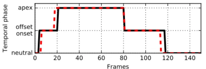
Fig. 2. The ground-truth temporal segments ( ) and the corresponding predicted temporal phases ( ) for each of the frames of a video displaying AU12 using DDATW.
The subgradient of Equation 16 then becomes ∂Pm i,j K ij DCT W ∗ ∂Yi = m X j ∂ K ij DCT W ∗ ∂Yi + m X j ∂ K ji DCT W ∗ ∂Yi = 2 m X j ∂ K ij DCT W ∗ ∂Yi . (18)
Note that by setting∆i=I, Equation 16 becomes an ob-jective for learning transformations for multiple sequences via DCCA [2]. Finally, we note that any warping method can be used in place of DTW for inferring the warping matrices
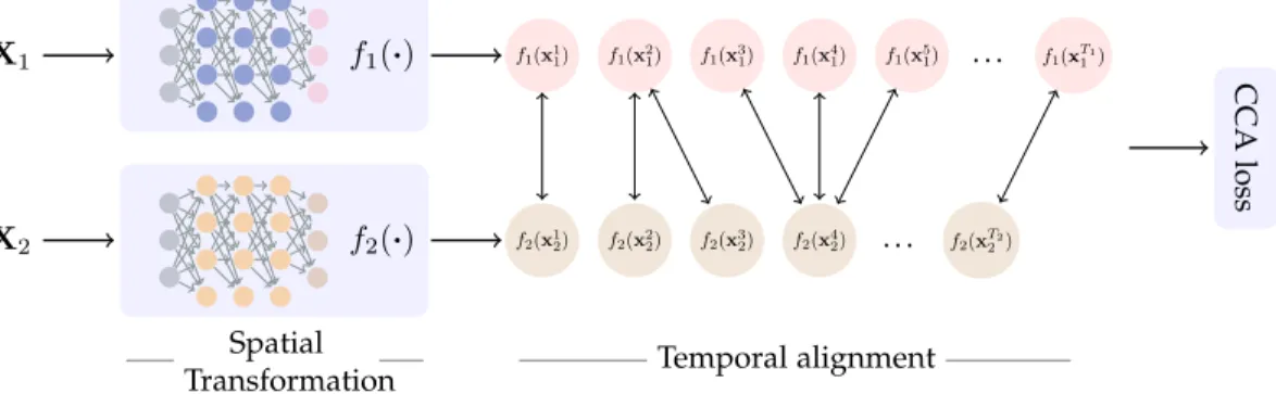
∆i(e.g., [44]), while DCTW is further illustrated in Figure 1.
3.1 Topology
At this point we should clarify that our model is topology-agnostic; our cost-function is optimised regardless of the number of layers or neuron type. Although we exper-imentally show later on that a 3-layer network can be sufficient, more elaborated topologies can be used that better suit the task-at-hand. An obvious example for this would be the problem of learning the optimal alignment and time-invariant representations of visual modalities such as videos. In this case, to reduce the free parameters of the model, convolutional neurons can be employed, and moreover the parameters for each networkfifor0< i < m can be tied (see Siamese networks [7]).
4
S
UPERVISEDD
EEPT
IMEW
ARPINGThe deep time-warping approach described in Section 3 recovers the appropriate non-linear transformations for temporally aligning a set of arbitrary sequences (e.g., temporally aligning videos of subjects performing the same, or similar, facial expression). This is done by optimizing an appropriate loss function (Equation 17). Nevertheless, in many similar problem settings, a set of labels characterising the temporal information contained in the sequences is readily available (e.g., labels containing the temporal phase of facial Action Units activated in the video). Although such labels can be readily utilised in order to evaluate the resulting alignment, this information remains unexploited in DCTW, as well as in other state-of-the-art time-warping methods such as [40], [43], [45].
In this section, we exploit the flexibility of the opti-misation problem proposed for DCTW in order to exploit
X1 X2 f1(·) f2(·) f1(x11) f1(x21) f1(x31) f1(x41) f1(x51) f2(x12) f2(x22) f2(x32) f2(x42) · · · · · · f1(xT11) f2(xT22) CCA loss Spatial
Transformation Temporal alignment
Fig. 1. Illustration of the DCTW architecture with two networks, one for each temporal sequence. The model is trained end-to-end, first performing a spatial transformation of the data samples and then a temporal transformation such as the temporal sequences are maximally correlated.
labelled information with the goal of enhancing perfor-mance on unseen, unlabelled data. By considering the set-ting where the sequences at-hand are annotated with dis-crete labels corresponding to particular temporal events, we firstly show that by appropriately modifying the objective for DCCA, we arrive at a numerically stable, non-linear vari-ant of the traditionally used Linear Discriminvari-ant Analysis (LDA), which we call Deep Discriminant Analysis (DDA). While DDA can be straightforwardly applied within a gen-eral supervised learning context in order to learn non-linear discriminative transformations, we subsequently extend the proposed optimisation problem for DCTW (Equation 17) by incorporating time-warping in the objective function. This leads to the Deep Discriminant Analysis with Time Warping (DDATW) method, that can be utilised towards temporally aligning multiple sequences while exploiting label information.
4.1 Deep Discriminant Analysis
Let us assume a set of T samples xi is given, with a label yi ∈ {1, . . . , C} corresponding to each sample. The classical Linear Discriminant Analysis (LDA) [13] computes a linear transformation ofWthat maximises the dispersion of class means while minimising the within-class variance. A standard formulation of LDA is given by the following a trace optimisation problem,
arg max
W
tr(W>SbW) s.t.W>StW=I
(19) whereSb=Pi=Cnimim>i ,ni are the number of samples ini-th class andmi =n1i
P
yk=ixkthe corresponding mean.
Furthermore,St=XX>is the total scatter matrix.
In matrix notation the between class scatter matrix can be constructed as follows,
Sb=XG(G>G)−1G>X>
whereG∈Rn×c is an indicator matrix in whichPjgij =
1, gij ∈ {0,1}, andgij is 1 iff data sampleibelongs to class j, and0otherwise. ThusXGis a matrix of the group sums, andXG(G>G)−1is a matrix which weights the sums with the respective number of data samples of each class.
The theory developed in [10] showed that there is an equivalence between least-square and trace optimisation
problems. In particular, the problem of finding the optimal
Wthat maps the data to labels can be written as
arg min
W
k(G>G)−12(G>−W>X)k2
F
The above is equivalent to finding the optimalWfrom the following trace optimisation problem
arg max
W
tr[W>XG(G>G)−1G>X>W]
s.t.W>XX>W=I, (20) which is precisely the problem formulation for LDA (Equa-tion 19).
As the connection between CCA (Equation 5) and LDA (Equation 20) is now established, we can easily extend LDA to a non-linear, hierarchical discriminant counterpart by taking advantage of the DCCA problem formulation in Equation 10. In more detail, the optimisation problem for Deep Discriminant Analysis (DDA) can be formulated as
arg min θ kf(X;θ)−(G>G)−12G>k2 F subject to:f(X;θ)f(X;θ)>=I, fp(X;θ)1=0,
or equivalently by using the trace norm formulation as
arg max
θ
kKLDAk∗, (21)
where KLDA = Σ˜LDA−
1/2 11 Σ˜LDA12 Σ˜ LDA−1/2 22 , ˜ ΣLDA 12 = 1 T−1X˜iCTG(G >G)−1 2, Σ˜LDA 22 =G(G>G)−1G>, ˜ ΣLDA 11 =T1−1X˜iCTX˜ > i with X˜i = fi(Xi;θi), while
CT = I− T111> denotes the centring matrix. We note that a Deep Linear Discriminant Analysis method has been recently proposed in [11], using a direct application of the LDA optimisation problem based on covariance diagonalisation, an approach that the authors found to be quite numerically unstable. On the contrary, the proposed DDA transformations based on (Equation 21) are found in a similar manner as DCCA, that is by using the sub-gradients of the nuclear norm, a process that involves computing the SVD. This approach can be more stable since the SVD decomposition exists for any matrix, not just for matrices that can be diagonalised.
4.2 Deep Discriminant Analysis with Time Warpings
The Deep Discriminant Analysis (DDA) method proposed in the previous section involves the optimisation of a trace norm in a similar manner to DCCA. DDA can thus be extended to incorporate time warpings, resulting in the proposed Deep Discriminant Analysis with Time Warp-ings (DDATW). That is, we can incorporate warpWarp-ings by simply replacing X˜i with X˜i∆i and (G>G)−
1
2G> with (G>G)−12G>∆gin Equation 21. In essence, we are solving
an equivalent problem to the one described in Equation 14, namely arg min ∀k.θk,∆k m X i,j=1 kfi(Xi;θi)∆i−(G>G)− 1 2G>∆jk2 F subject to:∀k.fk(Xk;θk)∆k∆>kfk(Xk;θk)>=I, ∀i, j.fi(Xi;θi)∆i∆>jfj(Xj;θj) =D, ∀k.fkp(Xk;θk)∆k1=0, ∀k.∆k∈ {0,1}Tk×T. (22) This formulation becomes particularly useful in cases when tackling tasks where discrete, temporal labels are available, for example, in case of annotating the temporal segments of the activations of facial Action Units (AUs). In particular, since in the vast majority of cases such labels are obtained by manually annotating the videos at hand, it is likely that artifacts such as lags and misalignments between labels and features may arise (e.g., an annotation that indicates that a particular AU has reached the apex phase after the actual phase has been actually reached in the video). In this case, the problem described in Equation 22 finds the appropriate non-linear transformation that maps the input features to thealigned temporal labels. Furthermore, another example of utilising the proposed DDATW formulation lies in set-tings where the alignment of multiple sequences is required while at the same time, discrete temporal labels are readily available. In this scenario, we can obtain the appropriate non-linear, discriminative transformation during training, by utilising the provided labels5. Given an out-of-sample
sequence during testing, we can then extract the non-linear transformations (learned while utilising labels available during training by solving Equation 22) and subsequently estimate the optimal time-warpings (∆i) that align the out-of-sample sequences to the learnt discriminative subspace.
5
E
XPERIMENTSIn order to assess the performance of DCTW, we perform de-tailed experiments against both linear and non-linear state-of-the-art temporal alignment algorithms. In more detail we compare against:
State of the art methods for time warping without a feature extraction step:
• Dynamic Time Warping (DTW) [33] which finds the
optimal alignment path given that the sequences reside in the same manifold (as explained in subsec-tion 2.2).
5. If the labels for any subsetKof available sequences are considered to be aligned with the corresponding features, then we can simply set
∀i.∆i=Iwherei∈ K.
• Iterative Motion Warping (IMW) [21] alternates
be-tween time warping and spatial transformation to align two sequences.
State-of-the art methods with a linear feature extractor:
• Canonical Time Warping (CTW) [43] as posed in sec-tion subsecsec-tion 2.2, CTW finds the optimal reduced dimensionality subspace such that the sequences are maximally linearly correlated.
• Generalized Time Warping (GTW) [44] which uses a combination of CTW and a Gauss-Newton temporal warping method that parametrises the warping path as a combination of monotonic functions.
State-of-the-art methods with non-linear feature extraction process.
• Manifold Time Warping [40] that employs a variation of Laplacian Eigenmaps to non-linearly transform the original sequences.
We evaluate the aforementioned techniques on four different real-world datasets, namely (i) the Weizmann database subsection 5.2, where multiple feature sets are aligned , (ii) the MMI Facial Expression database subsec-tion 5.3, where we apply DCTW on the alignment of facial Action Units,(iii)the XRMB database subsection 5.4 where we align acoustic and articulatory recordings, and finally
(iv) the CUAVE database subsection 5.5, where we align visual and auditory utterances.
Evaluation For all experiments, unless stated
oth-erwise, we assess the performance of DCTW utilising the the alignment error introduced in [44]. Assuming we have m sequences, each algorithm infers a set of warping paths Palg=
h
palg1 ,palg2 , . . . ,palgm
i
, where pi ∈
x∈Nlalg|1≤x≤n
m is the alignment path for the ith sequence with a lengthlalg. The error is then defined as
Err=dist(P alg
,Pground) + dist(Pground,Palg)
lalg+lground , distP1,P2= l1 X i=1 minl2 j=1 p 1 (i)−p 2 (j) 2. 5.1 Experimental Setup
In each experiment, we perform unsupervised pretraining of the deep architecture for each of the available sequences in order to speed up the convergence of the optimisation procedure. In particular, we initialise the parameters of each of the layers using a denoising autoencoder [39]. We utilise full-batch optimisation with AdaGrad [12] for training, al-though similar results are obtained by utilising mini-batch stochastic gradient descent optimisation with a large mini-batch size. In contrast to [2], we utilise a leaky rectified linear unit witha= 0.03(LReLU) [26], wheref(x) = max(ax, x)
and a is a small positive value. In our experiments, this function converged faster and produced better results than the suggested modified cube-root sigmoid activation func-tion. For all the experiments (excluding subsection 5.2 where a smaller network was sufficient) we utilised a fixed three layer 200–100–100 fully connected topology, thus reducing the number of free hyperparameters of the architecture.
This both facilitates the straight-forward reproducibility of experimental results, as well as helps towards avoiding overfitting (particularly since training is unsupervised).
5.2 Real Data I: Alignment of Human Actions under Multiple Feature Sets
In this experiment, we utilise the Weizmann database [17], containing videos of nine subjects performing one of ten actions (e.g., walking). We adopt the experimental proto-col described in [44], where 3 different shape features are computed for each sequence, namely(1)a binary mask,(2)
Euclidean distance transform [28], and (3) the solution of the Poisson equation [16], [44]. Subsequently, we reduce the dimensionality of the frames to 70–by–35 pixels, while we keep the top 123 principle components. For all algorithms, the same hyperparameters as [44] are used. Following [43], [44], 90% of the total correlation is kept, while we used a topology of two layers carrying 50 neurons each. Triplets of videos where subjects are performing the same action where selected, and each alignment algorithm was evaluated on aligning the three videos based on the features described above. pDTW pDDTW pIMW pCTW GTW DCTW 0.5 1.0 1.5 2.0 2.5 3.0 3.5 4.0
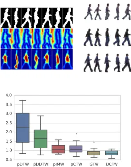
Fig. 3. Aligning sequences of subjects performing similar actions from the Weizmann database. (left) the three computed features for each of the sequences (1) binary (2) euclidean (3) poisson solution. (middle) The aligned sequences using DCTW. (right) Alignment errors for each of the six techniques.
The ground truth of the data was approximated by run-ning DTW on the binary mask images. Thus, the reasorun-ning behind this experiment is to evaluate whether the methods manage to find a correlation between the three computed features, in which case they would find the alignment path produced by DTW.
In Figure 3 we show the alignment error for ten ran-domly generated sets of videos. As DTW, DDATW, IMW, and CTW are only formulated for performing alignment be-tween two sequences we use their multi-sequence extension
as formulated in [45] and we use the prefixpto denote the multisequence variant.
We observe that DTW and DDTW fail to align the videos correctly, while CTW, GTW, and DCTW perform quite better. This can be justified by considering that DTW and DDTW are applied directly on the observation space, while CTW, GTW and DCTW infer a common subspace of the three input sequences. The best performing methods are clearly GTW and DCTW.
5.3 Real Data II: Alignment of Facial Action Units
Next, we evaluate the performance of DCTW on the task of temporal alignment of facial expressions. We utilise the MMI Facial Expression Dataset [31] which contains more than 2900 videos of 75 different subjects, each performing a particular combination of Action Units (i.e., facial muscle activations). We have selected a subset of the original dataset which contains videos of subjects which manifest the same action unit (namely, AU12which corresponds to a smile), and for which we have ground truth annotations. We preprocessed all the images by converting to greyscale and utilised an off-the-shelf face detector along with a face alignment procedure [23] in order to crop a bounding box around the face of each subject. Subsequently, we reduce the dimensionality of the feature space to 400 components using whitening PCA, preserving 99% of the energy. We clarify that the annotations are given for each frame, and describe the temporal phase of the particular AU at that frame. Four possible temporal phases of facial action units are defined:neutralwhen the corresponding facial muscles are inactive,onsetwhere the muscle is activated,apexwhen facial muscle intensity reaches its peak, andoffsetwhen the facial muscle begins to relax, moving towards the neutral state. Utilising raw pixels, the goal of this experiment lies in temporally aligning each pair of videos. In the context of this experiment, this means that the subjects in both videos exhibit the same temporal phase at the same time. E.g., for smiles, when subject 1 in video 1 reaches the apex of the smile, the subject in video 2 does so as well. In order to quantitatively evaluate the results, we utilise the ratio of correctly aligned frames within each temporal phase to the total duration of the temporal phase across the aligned videos. This can be formulated as|Φ1∩Φ2|
|Φ1∪Φ2|, whereΦ1,2is the
set of aligned frame indices after warping the initial vector of annotations using the alignment matrices ∆i found via a temporal warping technique.
Results are presented in Figure 4, where we illustrate the alignment error on 45 pairs of videos across all methods and action unit temporal phases. Clearly, DTW overperforms MW, while CCA based methods such as CTW and GTW perform better than DTW. It can be seen that the best performance in all cases is obtained by DCTW, and using at-test with the next best method we find that the result is statistically significant (p < 0.05). This can be justified by the fact that the non-linear hierarchical structure of DCTW facilitates the modelling of the complex dynamics straight from the low-level pixel intensities.
Furthermore, in Figure 5 we illustrate the alignment results from a pair of videos of the dataset. The first row depicts the first sequence in the experiment, where for each
DTW MTW IMW CTW GTW DCTW 0.0 0.1 0.2 0.3 0.4 0.5 0.6 0.7 Neutral DTW MTW IMW CTW GTW DCTW Onset DTW MTW IMW CTW GTW DCTW Apex DTW MTW IMW CTW GTW DCTW Offset DTW MTW IMW CTW GTW DCTW Mean
Fig. 4. Temporal phase detection accuracy as defined by the ratio of correctly aligned frames with respect to the total duration for each temporal phase – the higher the better.
Neutral Offset Apex Onset Neutral
GTW CTW DCTW Ground T ruth neutral neutral neutral neutral neutral neutral neutral neutral onset onset onset onset offset offset offset offset apex apex apex apex
neutral onset apex offset neutral
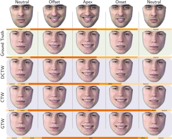
Fig. 5. Facial expression alignment of videosS002–005andS014–009from MMI dataset (subsection 5.3). Depicted frames for each temporal phase with duration[ts, te]correspond to the middle of each of the temporal phase,tc =dts+2tee. We also plot the temporal phases ( neutral,
onset, apex, and offset) corresponding to (i) the ground truth alignment and (ii) compared methods (DCTW, CTW and GTW). Note that the entire video is included in our supplementary material.
temporal phase with duration [ts, te] we plot the frame tc = dts+2tee. The second row illustrates the ground truth of the second video, while the following rows compare the alignment paths obtained by DCTW, CTW and GTW respec-tively. By observing the corresponding images as well as the temporal phase overlap, it is clear that DCTW achieves the best alignment. At last we repeat the experiment using a convolutional network topology which operates directly on the raw image pixel intensities. We opted for a simple architecture similar to LeNet [35], consisting of 2 convolu-tional layers of 32 filters each (kernel size 3) followed by a 2x2 max-pooling operation and finally a linear projection to 10 dimensions. Although this architecture attains the same performance in terms of accuracy, we found that (i) the optimisation converged quicker, and (ii) we obtained interpretable features which show the inner-workings of the network shown in Figure 6.
Fig. 6. Depicted are the last convolutional features (bottom row) using a 3-layer architecture showing frames from a video (top row) containing AU12 (Lip Corner Puller). The features seem to activate on the presence of smile and squinting of the eyes.
5.4 Real Data III: Alignment of Acoustic and Articula-tory Recordings
The third set of experiments involves aligning simultaneous acoustic and articulatory recordings from the Wisconsin X-ray Microbeam Database (XRMB) [42]. The articulatory data
consist of horizontal and vertical displacements of eight pellets on the speaker’s lips, tongue, and jaws, yielding a 16-dimensional vector at each time point. We utilise the features provided by [2]. The baseline acoustic features consist of standard 13-dimensional mel-frequency cepstral coefficients (MFCCs) [8] and their first and second deriva-tives computed every 10ms over a 25ms window. For the articulatory measurements to match the MFCC rate, we concatenate them over a 7-frame window, thus obtaining
Xart∈R273andX
MFCC∈R112.
As the two views were recorded simultaneously and then manually synchronised [42], we use this correspon-dence as the ground truth and then we produce a synthetic misalignment to the sequences, producing 10 sequences of 5000 samples. We warp the auditory features using the alignment path produced by Pmis(i) = i1.1lMFCC0.1 for
1≤i≤lMFCCwherelMFCCis the number of MFCC samples.
Results are presented in Table 1. Note that DCTW out-performs compared methods by a much larger margin than other experiments here. Nevertheless, this is quite expected: the features for this experiment are highly heterogeneous and e.g., in case of MFCCs, non-linear. The multi-layered non-linear transformations applied by DCTW are indeed much more suitable for modelling the mapping between such varying feature sets.
DTW MTW IMW
63.52±27.06 94.42±13.20 83.23±0.11
CTW GTW DCTW
58.92±28.8 64.06±5.01 7.19±1.79
TABLE 1
Alignment errors obtained on the Wisconsin X-ray Microbeam Database.
5.5 Real Data IV: Alignment of Audio and Visual Streams
In arguably, our most challenging experimental setting, we aim to align the subject’s visual and auditory utterances. To this end, we use the CUAVE [32] database which contains 36 videos of individuals pronouncing the digits 0 to 9. In particular, we use the portion of videos containing only frontal facing speakers pronouncing each digit five times, and use the same approach as in subsection 5.4 in order to introduce misalignments between the audio and video streams. In order to learn the hyperparameters of all em-ployed alignment techniques, we leave out 6 videos.
Regarding pre-processing, from each video frame we extract the region-of-interest (ROI) containing the mouth of the subject using the landmarks produced via [23]. Each ROI was then resized to 60 x 80 pixels, while we keep the top 100 principal components of the original signal. Subse-quently, we utilise temporal derivatives over the reduced vector space. Regarding the audio signal, we compute the Mel-frequency cepstral coefficients (MFCC) features using a 25ms window adopting a step size of 10ms between successive windows. Finally, we compute the temporal derivatives over the acoustic features (and video frames). To match the video frame rate, 3 continuous audio frames are concatenated in a vector. The results show that DCTW
DTW IMW MTW CTW GTW DCTW 0 10 20 30 40 50
Alignment Error
Fig. 7. Alignment errors on the task of audio-visual temporal alignment. Note that videos better illustrating the results are included in our supple-mentary material.
outperforms the rest of the temporal alignment methods by a large margin. Again, the justification is similar to subsec-tion 5.4: the highly heterogeneous nature of the acoustic and video features highlights the significance of deep non-linear architectures for the task-at-hand. It should be noted that the best results obtained for GTW utilise a combination of hyperbolic and polynomial basis, which biases the results in favour of GTW due to the misalignment we introduce. Still, it is clear that DCTW obtains much better results in terms of alignment error.
5.6 Deep Discriminant Analysis with Time Warpings (DDATW)
We perform two additional experiments in order to evaluate the proposed Deep Discriminant Analysis (Section 4), where in this case our data will also consist of a set of labels corresponding to the samples at-hand. In our first experi-ment, we utilise set of videos described in subsection 5.3 from the MMI database, that display facial expressions. In more detail, we exploit the fact that the action units have been labelled with regards to the temporal phases of facial behaviour (similarly to the setting for the experiment described in subsection 5.3.) Since each frame of the video has been assigned to a temporal phase, we utilise these labels in order to evaluate the proposed DDA. In particular, during training we utilise the available labels in order to learn the discriminant transformation. Subsequently, the learnt transformation can be applied to testing data in order to predict the labels. An example of the temporal segment annotations and the corresponding prediction for AU12 (Lip Corner Puller) can be found in Figure 2.
For our second experiment, we utilise the temporal labels available for the CUAVE dataset (as described in subsection 5.5). Since in each video a subject is uttering the digits 1 to 10, each framed is labelled with respect to whether the subject is uttering a digit or not. If the subject is uttering a digit, then the corresponding class corresponds to the particular digit being uttered. If not, then the frame is classified separately. This leads to 11 classes in total. For this experiment, we utilise half the data for training/validation and the other half for testing. The results are summarised in Table 2, where we compare between the unsupervised CTW and DCTW, as well as the proposed Deep Discriminant Analysis with Time Warpings (DDATW), as well as the
linear version of DDATW, which we term DATW. Note that by introducing supervision, we are able to further improve results.
TABLE 2
Classification accuracy using the available temporal phase labels for MMI (3 labels) and the digit annotations for CUAVE (11 labels).
CTW DATW DCTW DDATW MMI 49.2 53.5 59.1 65.1
CUAVE 35.7 43.6 68.7 83.7
6
C
OMPUTATIONAL DETAILS AND DISCUSSION The computational complexity of aligning a set of m se-quences each of length Ti is O(Pm i,jTiTj+ Pm i=1d 3 i) per iteration of the algorithm, which is the complexity of DTW plus the cost of the SVD in the computation of the deriva-tives in Equation 15. As the SVD is performed on the last layer of the network, which is of reduced dimensionality (di = 100 units in our case) it is relatively cheap. In contrast other non-linear warping algorithms [40] require an expensive k-nearest neighbour search accompanied by an eigendecomposition step or, in the case of CTW [43], an eigendecomposition of the original covariance matrices which becomes much more expensive when dealing with data of high dimensionality. Nevertheless, the proposed algorithm may require to perform more iterations in order to converge than CTW. In particular, DCTW needed around 5 minutes to converge in our second experiment subsec-tion 5.3 of aligning facial acsubsec-tion units, while for the same experiment CTW required around 1 minute. A way to expedite the procedure is to apply linear approximations of DTW such as [34], [44] or optimise the alignment paths only on a subset of iterations (this is an interesting line of further research on the topic).
Finally, it is worthwhile to mention that although in this work we explored simple network topologies, our cost function can be optimised regardless of the number of layers or neuron type (e.g., convolutional). Finally we also note that DCTW is agnostic to the use of the method for tempo-rally warping the sequences and other relaxed variants of DTW might be employed in practise when there is a large number of observations in each sequence as for example Fast DTW [34] or GTW [44] as long as it conforms to the alignment constrains, i.e., it always minimises the objective function.
7
C
ONCLUSIONSIn this paper, we study the problem of temporal alignment of multiple sequences. To the best of our knowledge, we propose the first temporal alignment method based on deep architectures, which we dub Deep Canonical Time Warping (DCTW). DCTW discovers a hierarchical non-linear fea-ture transformation for multiple sequences, where (i) all transformed features are temporally aligned, and (ii) are maximally correlated. Furthermore, we consider the setting where temporal labels are provided for the data-at-hand. By modifying the objective function for the proposed method,
we are able to provide discriminant feature mappings that may be more suitable for classification tasks. Finally, by means of various experiments on several datasets, we high-light the significance of the proposed methods on various applications, as the proposed method outperforms com-pared state-of-the-art methods.
A
CKNOWLEDGMENTSGeorge Trigeorgis is a recipient of the fellowship of the Department of Computing, Imperial College London, and this work was partially funded by it. The work of Ste-fanos Zafeiriou was partially funded by the EPSRC project EP/J017787/1 (4D-FAB), as well as by the FiDiPro pro-gram of Tekes (project number: 1849/31/2015). The work of Bj ¨orn W. Schuller was partially funded by the European Community’s Horizon 2020 Framework Programme under grant agreement No. 645378 (ARIA-VALUSPA). The respon-sibility lies with the authors.
George Trigeorgishas received an MEng in Ar-tificial Intelligence in 2013 from the Department of Computing, Imperial College London, where he is currently completing his Ph.D. studies. He was a recipient of the prestigious Google Ph.D. Fellowship in Machine Perception for 2017. He has regularly published in several prestigious conferences in his field including ICML, NIPS, and IEEE CVPR, while he is also a reviewer in IEEE T-PAMI, IEEE CVPR/ICCV/FG.
Mihalis A. Nicolaou is a Lecturer at the
De-partment of Computing at Goldsmiths, University of London and an Honorary Research Fellow with the Department of Computing at Imperial College London. Mihalis obtained his PhD from the same department at Imperial, while he com-pleted his undergraduate studies at the Depart-ment of Informatics and Telecommunications at the University of Athens, Greece. Mihalis’ re-search interests span the areas of machine learning, computer vision and affective comput-ing. He has been the recipient of several awards and scholarships for his research, including a Best Paper Award at IEEE FG, while publishing extensively in related prestigious venues. Mihalis served as a Guest Associate Editor for the IEEE Transactions on Affective Computing and is a member of the IEEE.
Stefanos Zafeiriou is currently a Senior Lec-turer in Pattern Recognition/Statistical Machine Learning for Computer Vision with the Depart-ment of Computing, Imperial College London, London, U.K, and a Distinguishing Research Fel-low with University of Oulu under Finish Distin-guishing Professor Programme. He was a recip-ient of the Prestigious Junior Research Fellow-ships from Imperial College London in 2011 to start his own independent research group. He was the recipient of the President’s Medal for Excellence in Research Supervision for 2016. He has received vari-ous awards during his doctoral and post-doctoral studies. He currently serves as an Associate Editor of the IEEE Transactions on Cybernet-ics the Image and Vision Computing Journal. He has been a Guest Editor of over six journal special issues and co-organised over nine workshops/special sessions on face analysis topics in top venues, such as CVPR/FG/ICCV/ECCV (including two very successfully challenges run in ICCV13 and ICCV15 on facial landmark localisation/tracking). He has more than 2800 citations to his work, h-index 27. He is the General Chair of BMVC 2017.
Bj ¨orn W. Schuller received his diploma, doc-toral degree, habilitation, and Adjunct Teaching Professorship all in EE/IT from TUM in Mu-nich/Germany. At present, he is a Reader (Asso-ciate Professor) in Machine Learning at Imperial College London/UK, Full Professor and Chair of Complex & Intelligent Systems at the University of Passau/Germany, and the co-founding CEO of audEERING UG. Previously, he headed the Ma-chine Intelligence and Signal Processing Group at TUM from 2006 to 2014. In 2013 he was also invited as a permanent Visiting Professor at the Harbin Institute of Technology/P.R. China and the University of Geneva/Switzerland. In 2012 he was with Joanneum Research in Graz/Austria remaining an expert consultant. In 2011 he was guest lecturer in Ancona/Italy and visiting researcher in the Machine Learning Research Group of NICTA in Sydney/Australia. From 2009 to 2010 he was with the CNRS-LIMSI in Orsay/France, and a visiting scientist at Imperial College. He co-authored 500+ technical contributions (10,000+ citations, h-index = 49) in the field.
R
EFERENCES[1] J. Aach and G. Church. Aligning gene expression time series with time warping algorithms.Bioinformatics, 17:495–508, 2001. [2] G. Andrew et al. Deep Canonical Correlation Analysis. InICML,
volume 28, 2013.
[3] F. Bach. Consistency of trace norm minimization. JMLR, 9:1019– 1048, 2008.
[4] F. Bach and M. Jordan. A probabilistic interpretation of canonical correlation analysis. 2005.
[5] A. Bruderlin and L. Williams. Motion signal processing. In
SIGGRAPH, pages 97–104, 1995.
[6] Y. Caspi and M. Irani. Aligning non-overlapping sequences.IJCV, 48:39–51, 2002.
[7] S. Chopra, R. Hadsell, and Y. LeCun. Learning a similarity metric discriminatively, with application to face verification. In IEEE CVPR. IEEE, 2005.
[8] S. Davis and P. Mermelstein. Comparison of parametric represen-tations for monosyllabic word recognition in continuously spoken sentences.IEEE TASSP, 28, 1980.
[9] F. De La Torre. A least-squares framework for component analysis.
IEEE TPAMI, 34:1041–1055, 2012.
[10] F. De La Torre. A least-squares framework for component analysis.
IEEE TPAMI, 34(6):1041–1055, 2012.
[11] M. Dorfer, R. Kelz, and G. Widmer. Deep linear discriminant analysis.arXiv preprint arXiv:1511.04707, 2015.
[12] J. Duchi et al. Adaptive Subgradient Methods for Online Learning and Stochastic Optimization.JMLR, 12:2121–2159, 2011.
[13] K. Fukunaga.Introduction to statistical pattern recognition. Academic press, 2013.
[14] R. Girshick et al. Rich feature hierarchies for accurate object detection and semantic segmentation. InIEEE CVPR, pages 580– 587. IEEE, 2014.
[15] D. Gong and G. Medioni. Dynamic Manifold Warping for view invariant action recognition. InIEEE CVPR, pages 571–578, 2011. [16] L. Gorelick et al. Shape representation and classification using the
poisson equation.IEEE TPAMI, 28:1991–2004, 2006.
[17] L. Gorelick et al. Actions as space-time shapes. IEEE TPAMI, 29:2247–2253, 2007.
[18] M. Hasan. On multi-set canonical correlation analysis. InIJCNN, pages 1128–1133. IEEE, 2009.
[19] G. Hinton et al. Deep neural networks for acoustic modeling in speech recognition: The shared views of four research groups.
IEEE Sig. Prog. Mag., 29(6):82–97, 2012.
[20] G. Hinton and R. Salakhutdinov. Reducing the dimensionality of data with neural networks.Science, 313:504–507, 2006.
[21] E. Hsu, K. Pulli, and J. Popovi´c. Style translation for human motion. InSIGGRAPH, volume 24, page 1082, 2005.
[22] B.-H. F. Juang. On the hidden markov model and dynamic time warping for speech recognitiona unified view. AT&T Bell Laboratories Technical Journal, 63(7):1213–1243, 1984.
[23] V. Kazemi and S. Josephine. One Millisecond Face Alignment with an Ensemble of Regression Trees. InIEEE CVPR, 2014.
[24] Y. Kim, H. Lee, and E. M. Provost. Deep learning for robust feature generation in audiovisual emotion recognition. InIEEE ICASSP, pages 3687–3691. IEEE, 2013.
[25] A. Krizhevsky et al. Imagenet classification with deep convolu-tional neural networks. InNIPS, pages 1097–1105, 2012.
[26] A. Maas et al. Rectifier nonlinearities improve neural network acoustic models. InICML, volume 30, 2013.
[27] K. Mardia et al.Multivariate analysis. Academic press, 1979. [28] C. Maurer and V. Raghavan. A linear time algorithm for
com-puting exact Euclidean distance transforms of binary images in arbitrary dimensions.IEEE TPAMI, 25:265–270, 2003.
[29] J. Ngiam, A. Khosla, and M. Kim. Multimodal deep learning.
ICML, 2011.
[30] A. A. Nielsen. Multiset canonical correlations analysis and mul-tispectral, truly multitemporal remote sensing data. IEEE TIP, 11(3):293–305, 2002.
[31] M. Pantic et al. Web-based database for facial expression analysis. InICME, volume 2005, pages 317–321, 2005.
[32] E. Patterson et al. CUAVE: A new audio-visual database for multimodal human-computer interface research. ICASSP, 2:II– 2017–II–2020, 2002.
[33] L. Rabiner and B. Juang. Fundamentals of Speech Recognition, volume 103. 1993.
[34] S. Salvador and P. Chan. Fastdtw: Toward accurate dynamic time warping in linear time and space. InKDD-Workshop, 2004. [35] B. Sch ¨olkopf and A. J. Smola. Learning with kernels: support vector
machines, regularization, optimization, and beyond. MIT press, 2002. [36] S. Shariat and V. Pavlovic. Isotonic CCA for sequence alignment
[37] Y. Taigman et al. Deepface: Closing the gap to human-level performance in face verification. InIEEE CVPR, pages 1701–1708. IEEE, 2014.
[38] G. Trigeorgis, M. Nicolaou, S. Zafeiriou, and B. W. Schuller. Deep Canonical Time Warping. InCVPR, 2016.
[39] P. Vincent et al. Stacked Denoising Autoencoders: Learning Use-ful Representations in a Deep Network with a Local Denoising Criterion.JMLR, 11:3371–3408, 2010.
[40] H. Vu et al. Manifold Warping: Manifold Alignment over Time. In
AAAI, 2012.
[41] A. Wang, J. Lu, G. Wang, J. Cai, and T.-J. Cham. Multi-modal unsupervised feature learning for RGB-D scene labeling. InECCV, pages 453–467. Springer, 2014.
[42] J. Westbury et al. X-ray microbeam speech production database.
JASA, 88(S1):S56—-S56, 1990.
[43] F. Zhou and F. De La Torre. Canonical time warping for alignment of human behavior.NIPS, 2009.
[44] F. Zhou and F. De La Torre. Generalized time warping for multi-modal alignment of human motion. InIEEE CVPR, pages 1282– 1289, 2012.
[45] F. Zhou and F. De La Torre. Generalized Canonical Time Warping.