2009, Vol. 52, No. 3, 307-320
OPTIMAL POLICY FOR A SIMPLE SUPPLY CHAIN SYSTEM WITH DEFECTIVE ITEMS AND RETURNED COST UNDER SCREENING
ERRORS
Tien-Yu Lin
Overseas Chinese University
(Received May 5, 2008; Revised December 22, 2008)
Abstract Recently, one of the most interesting topics in supply chain management (SCM) is the integrated vendor-buyer production-inventory problem, in which the critical issue is to determine economic lot size per shipment and deliveries. Most researches on this issue assume that products are screened and the process is perfect; however, screening errors (including type-I and type-II) may occur with imperfect quality in practice. In this paper we consider a simple single-vendor single-buyer supply chain system in which products are received with defective quality, and 100% screening process is performed with possible inspection errors. The objective of this paper is to determine the optimal number of shipments as well as the size of each shipment in order to minimize the joint annual cost incurred by both vendor and buyer. We develop a cost model for the supply chain system and propose a solution procedure to find the optimal solution. A numerical example is given to illustrate the application of the model. Besides, based on the numerical example, a sensitivity analysis is also made to investigate the effects of five important parameters (the inspection rate, the annual demand, the defective rate, Type I error, and Type II error) on the optimal solution.
Keywords: Inventory, supply chain, screening error, shipment, imperfect quality 1. Introduction
Recently, the issue of just-in-time (JIT) manufacturing has received considerable attention, and one of the most interesting topics on this issue is the integration of vendor and buyer in the supply chain system [4]. Many researches have shown that improved benefits can be achieved through the coordination of vendor and buyer. In his pioneer work Goyal [9] considered the joint optimization problem of vendor and buyer, in which he assumed that vendor’s production rate was infinite. Banerjee [1] extended the result to the case of finite production rate, and developed a joint economic lot size (JELS) model in which vendor made to order under lot-for-lot policy. Goyal [10] further relaxed the lot-for-lot assumption, and proposed a model in which each production batch was shipped to buyer in smaller batches of equal size. Later Hill [15] established an optimal batching and shipment policy; in his work, he showed that the successive shipment sizes of the first m shipments should be adjusted by a fixed factor and the remaining shipments should be equal-sized. Ha and Kim [13] used geometric programming model to integrate decisions of vendor and buyer, in which small production lots were considered. Hoque and Goyal [16] proposed an optimal procedure to a single-vendor, single-buyer production and inventory problem with both equal and unequal sized shipments, in which capacity constraint of transportation equipments was considered. Later Pan and Yang [21] investigated an integrated inventory model with controllable lead time with normally distributed demand. Recently, Buscher and Lindner [3] presented a lot size model to allow the simultaneous determination of production as well as rework lot
and batches. In the same time, Ertogral et al. [8] analyzed the lot-sizing problem under equal-sized shipment policy, in which they incorporated transportation cost explicitly into the model.
Based on the model of equal-size sub-batches shipments to buyer, Goyal [11] proposed the use of unequal-sized sub-batches in which he suggested that the ith shipment size to buyer within a production batch should be adjusted accordingly. Hill [14] extended this idea and proposed general shipment sizes that were increased by a general fixed factor, ranging from 1 to the ratio between the production rate and demand rate. Viswanathan [27] showed that neither the policy with equal-sized batches nor the policy with unequal-sized sub-batches dominated each other. Bogaschewsky et al. [2] presented a model for a multi stage production/inventory system in which a uniform lot size is produce through all stages and partial lot size may be transported to the next stages upon completion. Recently, Hoque and Goyal [17] developed an alternative generalized model in which equal and unequal batch shipments of a lot from the vendor to the buyer is considered.
However, many researchers pointed out that the issue of defective items or imperfect quality was of practical importance. Porteus [23] incorporated the effect of imperfect items into the basic EOQ model, in which he developed a simple model to illustrate the relationship between quality and lot size. Rosenblatt and Lee [24] assumed the defective items could be reworked at a cost, and they found that defective items motivated smaller lot size. Later, Schwaller [26] assumed that defective items were present in incoming lots so that inspection costs should be incurred due to such items. Cheng [6] developed an EOQ model with demand-dependent unit production cost and imperfect production processes; in his work, he formulated the inventory decision problem as a geometric programming model. Zhang and Gerchak [29] also integrated lot sizing and inspection policy in an EOQ model, in which they assumed that a random proportion of items were defective. Later Yang and Wee [28] employed an integrated approach to determine economic ordering policy of deteriorated item. Under the assumption that defective items could be sold as a single batch by the end of 100% screening process, Salameh and Jaber [25] developed an EOQ-based model for items received with imperfect quality; in their work, they found that the economic lot size increased as the average percentage of defective items increased. Goyal and Cardenas-Baeeon [12] developed a simple method to determine the economic production quantity for items with imperfect quality. Recently Huang [19] incorporated the integrated method and the process unreliability into the production-inventory model. Based on the work of Huang [19], Chung [7] developed a necessary and sufficient condition for the existence of the optimal solution to complete and improve the solution procedure of Huang’s work. Papachristors and Konstantaras [22] further discussed the issue of non-shortages in inventory models with imperfect quality. More recently, Hsu et al. [18] developed a deteriorating inventory replenishment model and presented an algorithm to derive both vendor’s managing cost and buyer’s optimal replenishment cycle, shortage period, as well as order quantity; in which they demonstrated that buyer’s profit was highly influenced by vendor’s lead time. Chen and Kang [5] developed the integrated vendor-buyer cooperative inventory models with the permissible delay in payments to determine the optimal replenishment time interval and replenishment frequency. More recently, Maddah and Jaber [20] rectified a flaw in an economic order quantity (EOQ) model with unreliable supply, characterized by a random fraction of imperfect quality items and a screening process, developed by Salameh and Jaber [25]. In their work, several batches of imperfect quality items to be consolidated and shipped in one lot are also discussed.
re-searches neglect the effect of screening errors when items need to be inspected. In practice it is often the case that, when 100% screening process is performed, inspection fails to be perfect due to Type I and Type II errors. Type I error occurs if perfect items are mistakenly classified as defective, and it results in unnecessarily requiring more items with extra cost; Type II error appears if imperfect items are mistakenly identified as perfect, and it incurs penalty cost. The objective of this paper is to extend the model developed by Huang [19] to the case with screening errors. More specifically, we consider the production and inventory model with imperfect quality under screening errors in which 100% screening process is realized.
This paper is organized as follows. In section 2, notations and assumptions used in this paper are given. Section 3 develops an integrated production and inventory model with defective items under screening errors. Section 4 gives a numerical example and conducts sensitivity analysis for the screening rate, annual demand, defective percentage, Type I error, and Type II error. Conclusion is summarized in section 5.
2. Notation and Assumptions
The following notations and assumptions are adapted in developing the integrated produc-tion and inventory model considered in this paper.
Parameters:
d unit screening cost
F transportation cost per shipment hB buyer’s annual holding cost per item hV vendor’s annual holding cost per item
m buyer’s penalty cost to replace one defective item returned by end-consumers SV vendor’s setup cost per production run
SB buyer’s ordering cost of placing an order v vendor’s unit warranty cost of defective items D annual demand
P annual production rate, P > D x screening rate
α Type I error, false rejection of nondefectives resulting in the necessity of producing additional items
β Type II error, false acceptance of defectives resulting in that the products shipped to the end-consumers
Y percentage of defective items, a random variable f(y) probability density function of Y
Unknowns:
n total number of shipments per production lot, a positive integer Q number of items per shipment
Qp lot size per production run, in which Qp =nQ T time interval between successive shipments Tc cycle time, in which Tc =nT
T CB(n, Q) buyer’s annual total cost T CV(n, Q) vendor’s annual total cost
K(n, Q) annual integrated total cost
Assumptions:
1. the supply chain consists of a single vendor and a single buyer 2. demand for the item is constant over time
3. production rate is uniform and finite
4. successive deliveries are scheduled so that the next delivery arrives at the buyer when the stock from previous shipment has just been used up
5. the number of perfect items is at least equal to the demand during screening time 6. shortages are not allowed
7. time horizon is assumed to be infinite
8. the vendor delivers the “true” defective items in a single batch at the end of the buyer’s 100% screening process and thus warranty cost occurs
3. Mathematical Model
In his recent paper, Huang [19] considered a single-vendor, single-buyer supply chain system with imperfect products in the integrated production-inventory model. The inventory levels of Huang’s model for both the vendor and buyer were depicted in Fig. 1, and the annual total cost of the integrated model (including both the vendor and the buyer) was given by
K(n, Q) = (SV +SB)D n(1−Y)Q + F D (1−Y)Q + D(d+vY) (1−Y) + { Q 2 + (n−2)Q 2 (1− D (1−Y)P) } hV + { Q(1−Y) 2 + DQY x(1−Y) } hB (3.1)
where the costs in the right-hand side of Eq.(3.1) are setup cost, ordering cost, trans-portation cost, screening cost, warranty cost, vendor’s holding cost, and buyer’s holding cost, respectively.
In contrast to Huang’s model, we consider in this paper that 100% screening process is performed, in which imperfect quality under inspection errors may occur. Hence, the buyer’s inventory level of Huang’s model is modified asQ[1−Y(1−β)−α(1−Y)] units. To avoid possible shortages, we assume that during the screening time Y is restricted to the following condition:
Y(1−β) +α(1−Y)≤1−D
x (3.2)
Furthermore, the cycle time is given by nT, where T = Q[1−α−YD(1−α−β)]. Therefore, the vendor’s annual holding cost,shown as HCV, can be written as
HCV =hV { Q 2 + (n−2)Q 2 [ 1− D P {1−α−Y(1−α−β)} ]}
Let T CV (n, Q) denote the vendor’s annual total cost, then we have T CV (n, Q) = SVD nQ[1−α−Y (1−α−β)] +dD [ α+Y(1−α−β) 1−α−Y(1−α−β) ] +vD [ Y(1−β) 1−α−Y(1−α−β) ] +hV { Q 2 + (n−2)Q 2 [ 1− D P {1−α−Y(1−α−β)} ]} (3.3)
nQ/P
nT Time
The total depletion of the vendor’s inventory The total accumulation of
the vendor’s inventory
nQ Time Q/P nQ/P T1 T2 T Inventory level (Vendor) Q Q (1-y)Q Time nT Inventory level (Buyer)
Figure 1: Time-weighted inventory for vendor and buyer.
+dD " α+Y(1−α−β) 1−α−Y(1−α−β) # +vD " Y(1−β) 1−α−Y(1−α−β) # +hV ( Q 2 + (n−2)Q 2 " 1− D P {1−α−Y(1−α−β)} #) (3.3) where the costs in the right-hand side of Eq.(3.3) are setup cost, warranty cost for ”true” defective items, screening cost for defective items returned by buyer, and holding cost, respectively.
Similarly, the buyer’s annual holding cost, denoted asHCB, is given by
HCB = ( Q[1−α−Y(1−α−β)] 2 + DQ x " −1 + 1 1−α−Y(1−α−β) #) hB
Figure 1: Time-weighted inventory for vendor and buyer.
where the costs in the right-hand side of Eq.(3.3) are setup cost, warranty cost for “true” defective items, screening cost for defective items returned by buyer, and holding cost, respectively.
Similarly, the buyer’s annual holding cost, denoted as HCB, is given by
HCB = { Q[1−α−Y(1−α−β)] 2 + DQ x [ −1 + 1 1−α−Y(1−α−β) ]} hB
Then, the buyer’s annual total cost T CB(n, Q) is given by
T CB(n, Q) = SBD nQ[1−α−Y (1−α−β)] + F D Q[1−α−Y(1−α−β)] + dD 1−α−Y(1−α−β)+ βmDY 1−α−Y(1−α−β)
+ { Q[1−α−Y(1−α−β)] 2 + DQ x [ −1 + 1 1−α−Y(1−α−β) ]} hB (3.4)
where the costs in the right-hand side of Eq.(3.4) are ordering cost, transportation cost, screening cost, holding cost, and penalty cost, respectively. Therefore, by adding Eq.(3.3) and (3.4) (i.e., the vendor’s annual total cost T CV(n, Q) and the buyer’s annual total cost T CB(n, Q)), the annual total cost of Huang’s model can now be modified as follows:
K(n, Q) = (SV +SB)D nQ[1−α−Y (1−α−β)] + F D Q[1−α−Y (1−α−β)] +D(d{1 + [α+Y (1−α−β)]}+vY (1−β)) [1−α−Y (1−α−β)] + βDY m [1−α−Y (1−α−β)] +hV { Q 2 + (n−2)Q 2 [ 1− D P{1−α−Y(1−α−β)} ]} +hB { Q 2 [1−α−Y(1−α−β)] + DQ x [ −1 + 1 1−α−Y(1−α−β) ]} (3.5) or K(n, Q) = { (SV+SBD) nQ + F D Q + ( 2d+v(1−α)(1−β) 1−α−β ) D } 1 1−α−Y(1−α−β) + { βmD(1−α) (1−α−β) − (n−2)QDhv 2P + DQhB x } 1 1−α−Y(1−α−β) −dD−vD 1−β 1−α−β − βmD 1−α−β + (n−1)Q 2 hV − DQ x hB +Q[1−α−Y (1−α−β)] 2 hB (3.6)
Letf(y) be the probability density function of random variable Y, by taking the expec-tation of Eq.(3.6), the expected annual total cost EK(n, Q) is given by
K(n, Q) = { (SV +SB)D nQ + F D Q + ( 2d+v(1−α) (1−β) 1−α−β ) D } Ω + { βmD(1−α) (1−α−β) − (n−2)QDhv 2P + DQhB x } Ω −dD−vD 1−β 1−α−β − βmD 1−α−β + (n−1)Q 2 hV − DQ x hB +Q[1−α−E[Y] (1−α−β)] 2 hB, where Ω =E [ 1 1−α−Y (1−α−β) ] . (3.7) Note that when the screening process is perfect (i.e., α=0 and β=0), Eq.(3.7) reduces to Huang’s model; besides, when all items are perfect (i.e., no screening process is needed), Eq.(3.7) will reduce to the model of Ha and Kim [13].
The following property is needed in the derivation of the optimal solution for the expected annual total cost EK(n, Q).
Property 1 For fixed n, EK(n, Q) is convex in Q.
Proof. See Appendix A1.
According to Property 1, the optimal value ofQcan be determined by letting ∂EK∂Q(n,Q) = 0, which yields Q∗(n) = v u u u t 2DΩ ( SV+SB n +F ) (n−1)hV − 2DhxB +hB[1−α−E[Y](1−α−β)] + Ω [ 2DhB x − (n−2)DhV P ] (3.8)
Thus, the procedure of determining the optimal number of shipmentsn∗ and lot sizeQ∗
is summarized in the following theorem:
Theorm 1 (1−DΩ/P)>0 holds if and only if the optimal solution (n∗, Q∗) of EK(n, Q)
exists. Furthermore, if(1−DΩ/P)>0holds, the optimal solution (n∗, Q∗) can be expressed as follows: (1) If ∆ = {2DΩhB x + 2DΩhV P −hV − 2DhB x +hB[1−α−E[Y] (1−α−β)] } ≥ 0, the optimal shipments from the vendor to the buyer must satisfy as follows.
(n∗−1)n∗ ≤ (SV +SB) ∆
(1−DΩ/P)hVF ≤
n∗(n∗+ 1) (3.9)
Also, Q∗ =Q∗(n∗) which can be determined by Eq.(3.8). (2) If ∆ = { 2DΩhB x + 2DΩhV P −hV − 2DhB x +hB[1−α−E[Y] (1−α−β)] } < 0, the optimal solution of (n∗, Q∗) can be expressed as n∗=1 and Q∗ =Q∗(1).
Proof. See Appendix A2.
4. Numerical Example and Sensitivity Analysis
In this section, we use the example given by Huang [19] to illustrate the effectiveness of our modified model developed in the previous section. The parameters are as follows:
Production rate P = 160,000 units/year
Demand rate D= 50,000 units/year
Setup cost for vendor SV = $300/cycle
Ordering cost for buyer SB= $100/cycle
Holding cost for vendor hV = $2/unit/year
Holding cost for buyer hB = $5/unit/year
Transportation cost F = $25/delivery
Screening rate x= 175,200 units/year
Screening cost d= $0.5/unit
Warranty cost of “true” imperfect quality items v = $30/unit
In addition, we set the penalty cost m= $50/unit, Type I error α = 0.01, and Type II error β = 0.02.
Due to the property of uncertainty and the lack of sufficient data for the defective rate, we can not properly determine the distribution of defective rate. Therefore, in this paper, we follow the previous researchers (such as Huang [19], Maddah and Jaber [20], Papachristos and Konstantaras [22], Salameh and Jaber [25], etc.) by employing the uniform distribution
as the form of defective rate. That is, we assume that the percentage defective random variable Y is uniformly distributed withp.d.f. asf(y) = 20,0≤y≤0.05. Then, one has
E[Y] =∫00.0520ydy= 0.025 and
Ω = E[1−α−Y(11−α−β)]=∫00.051−α−y20(1−α−β)dy= 1.035682.
Further, we have ∆ = 4.225185≥0. Since(1−DPΩ)= 0.67635>0 and ∆ = 4.225185≥ 0, from Theorem 1, we have (SV+SB)∆
(1−DΩ/P)F hV = 49.97638. Thus, by Eq.(3.9), the optimal number of shipments is given by n∗ = 7. Furthermore, setting n∗ = 7 into Eq.(3.8), we have the optimal lot size per shipment Q∗ ≈788. Hence, the expected annual total cost is $77207.6. Compared with Huang [19], the number of shipments of our model is the same as that of Huang [19]; while the lot size of each shipment and the expected annual total cost of our model are larger than those of Huang [19].
Obviously, the optimal policy (including Q∗, N∗, and EK∗) for the proposed supply chain system is dependent on the parameters P, D, SV, SB, hV, hB, F, x, d, v, m, α, and β. A
complete investigation of the effect of these parameters on the optimal solution would be a laborious computational work. To reduce the computational labor, we take only x, D, U, α, and β into account. All of the five parameters are set at two levels. Their values are summarized as follows: x (1) 175200 (2) 350400 ; D (1) 50000 (2) 80000 ; U (1) 0.05 (2) 0.10 ; α (1) 0.01 (2) 0.03 ;β (1) 0.02 (2) 0.04 .
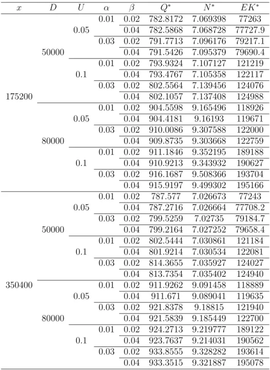
Except these five parameters, the other parameters are set as stated above. Table 1 lists the optimal solutions under 32 combinations of x, D, U, α, and β. From the table, we can get some findings described as follows:
1. Q∗ is increasing withx; whileN∗ andEK∗are decreasing withx. As to the increasing of
Q∗ withx, this is rather intuitive because a higher inspection rate leads to fast removal of defective items, which reduces the inventory holding cost and allows ordering more quantity. This result agrees with Maddah and Jaber’s work [20]. Consequently, the increasing of lot size in each shipment will lead directly to the increasing in the lengths of the time intervals between successive shipments. Hence, the number of shipments in each cycle will decrease. Finally, due to the decreases of the receiving and transportation costs resulting from the decrease ofN∗, we have that EK∗ will decrease asx increases. 2. Q∗,N∗, andEK∗ are all increasing withD. This is similar to the case in the traditional
EOQ model.
3. Q∗, N∗, andEK∗ are increasing inU. That is, the higher the defective rate, the higher the order quantities, the number of shipments, and the expected annual total cost are. Obviously, as the defective rate increases, the buyer needs more quantity per shipment to satisfy the demand. This result consists with the Salameh and Jaber’s [25] work. This increment in lot size will lead to extra shipments and costs. In contrast, the effect of the defective rate on the expected annual total cost is higher than those on the lot size per shipment and the number of shipments.
4. As expected, Q∗, N∗, and EK∗ are also increasing in α. This is because type I error will “reduce” the quantity of non-defectives in the lot size per shipment and then result in the necessity of increasing the lot size per shipment and/or the number of shipments to satisfy the demand.
5. Q∗ and N∗ are decreasing in β; while EK∗ is increasing in β. This can be understood by noting that false acceptance of defectives will inflate the quantity of non-defectives in the lot size per shipment, and hence decrease the lot size per shipment and the number of shipments. Next, naturally, false acceptance of defectives will incur much penalty cost and then decrease the expected annual total cost.
Table 1: The values ofQ∗ ,N∗ , andEK∗ corresponding to 32 combinations ofx,D,U,α, and β x D U α β Q∗ N∗ EK∗ 0.01 0.02 782.8172 7.069398 77263 0.05 0.04 782.5868 7.068728 77727.9 0.03 0.02 791.7713 7.096176 79217.1 50000 0.04 791.5426 7.095379 79690.4 0.01 0.02 793.9324 7.107127 121219 0.1 0.04 793.4767 7.105358 122117 0.03 0.02 802.5564 7.139456 124076 175200 0.04 802.1057 7.137408 124988 0.01 0.02 904.5598 9.165496 118926 0.05 0.04 904.4181 9.16193 119671 0.03 0.02 910.0086 9.307588 122000 80000 0.04 909.8735 9.303668 122759 0.01 0.02 911.1846 9.352195 189188 0.1 0.04 910.9213 9.343932 190627 0.03 0.02 916.1687 9.508366 193704 0.04 915.9197 9.499302 195166 0.01 0.02 787.577 7.026673 77243 0.05 0.04 787.2716 7.026664 77708.2 0.03 0.02 799.5259 7.02735 79184.7 50000 0.04 799.2164 7.027252 79658.4 0.01 0.02 802.5444 7.030861 121184 0.1 0.04 801.9214 7.030534 122081 0.03 0.02 814.3655 7.035927 124027 0.04 813.7354 7.035402 124940 350400 0.01 0.02 911.9262 9.091458 118889 0.05 0.04 911.671 9.089041 119635 0.03 0.02 921.8378 9.18815 121940 80000 0.04 921.5839 9.185449 122700 0.01 0.02 924.2713 9.219777 189122 0.1 0.04 923.7637 9.214031 190562 0.03 0.02 933.8555 9.328282 193614 0.04 933.3515 9.321887 195078
6. Wholly, from Table 1, it is also observed that none of the second order interactions of
x, D, U, α, andβis significant. That is, it seems that an additive model is appropriate to model the relationship between Q∗ (N∗ and EK∗) and the five parameters (x, D, U, α, and β).
5. Conclusion
In practice, based on the vendor-buyer coordination focusing on item flows with an objec-tive of minimizing supply chain costs, the vendor is usually required to deliver the items by lot-splitting shipments so as to minimize inventory holding cost for the buyer, as done in a long-term purchase agreement of a JIT manufacturing environment. In this paper, we propose a generalized production-inventory model in which items may be received with imperfect quality, screening errors and lot-splitting shipments. An analytic solution proce-dure is developed to compute the optimal total number of shipments and the size of each shipment. The works of Huang [19] and Ha and Kim [13] are two special cases of our model, associated with the cases with the screening process being perfect and all items being per-fect, respectively. An investigation of the effects of five important parameters (the inspection rate, the annual demand, the defective rate, Type I error, and Type II error) on the optimal solution is also made. Numerical results shows that (1) as the inspection rate increases, the optimal lot size per shipment increases; while the number of deliveries and the expected annual total cost decrease. (2) the higher the annual demand, the higher the optimal lot size per shipment, the number of deliveries and the expected annual total cost. (3) as the defective rate increases, the values of optimal lot size per shipment, number of deliveries and expected annual total cost increase. Besides, in contrast to the quantities per shipment and the number of deliveries, the defective rate has a larger effect on the expected annual total cost. (4) the higher the Type I error, the higher the optimal lot size per shipment, the number of deliveries and the expected annual total cost. (5) if Type II error increases, the value of optimal lot size per shipment and the number of deliveries decrease; while the expected annual total cost increases. Besides, the optimal quantities per shipment and the number of deliveries are rather robust to the moderate changes in type II error.
Appendix A1
Proof of Property 1.
Taking the first and second partial derivatives of EK(n, Q) with respect to Q, we have
∂EK(n, Q) ∂Q = { −(SV +SB)D nQ2 − F D Q2 − (n−2)DhV 2P + DhB x } Ω +(n−1) 2 hV − DhB x + hB[1−α−E[Y] (1−α−β)] 2 , (5.1) and ∂2EK(n, Q) ∂2Q = { 2D(SV +SB) nQ3 + 2F D Q3 } Ω>0 (5.2)
Therefore, for fixedn,EK(n, Q) is convex inQ. This completes the proof ofProperty 1. Appendix A2
Proof of Theorem 1.
EK(n) = √ 2D (S V +SB n +F ) Ωφ(n) + [ 2d+v(1−α) (1−β) 1−α−β ] D Ω +βmD(1−α) 1−α−β Ω−dD−vD (1−β) 1−α−β − βmD 1−α−β (5.3) whereφ(n) = [ 2DhB x −(n−2) DhV P ] Ω+(n−1)hV−2DhxB+hB[1−α−E[Y] (1−α−β)]
By ignoring the terms that are independent of n, taking square of EK(n), and then dividing by 2DΩ, we have EK(n) =nhVF ( 1− DΩ P ) +(SV +SB) ∆ n (5.4) where ∆ = 2DΩhB x + 2DΩhV P −hV − 2DhB x +hB[1−α−E[Y] (1−α−β)]
Taking the first derivative of EK(n) with respect to n, we get
dEK(n) dn =hVF ( 1− DΩ P ) −(SV +SB) ∆ n2 (5.5)
There are three cases, similar to Chung [7], to be discussed: • Case 1: (1−ΩD/P)>0
Taking the derivative of φ(n) with respect n, we have
dφ(n) dn =hV ( 1−DΩ P ) >0 (5.6)
Thus,φ(n) is increasing on [1,∞) and for all n ≥1, we have
φ(n)> φ(1) = 2DhB(Ω−1)
x +
DΩhV
P +hB[1−α−E[Y] (1−α−β)]>0 (5.7)
Furthermore, two scenarios may occur:
Scenario 1: ∆ ≥0 We here let ˆ n= v u u t (SV +SB) ∆ (1−ΩD/P)hVF (5.8) Thus, one has
dEK(n) dn <0, if 0< n <nˆ = 0, if n= ˆn >0, if n >ˆn (5.9)
Eq.(5.9) implies EK(n) is decreasing on (0,ˆn] and increasing on [ˆn,∞). Since n is a positive integer, the optimal value n∗ is obtained when
EK(ni∗)≤EK(ni∗ −1) and EK(ni∗)≤EK(ni∗+ 1) (5.10)
From Eqs.(5.4) and (5.10), n∗ satisfies the following condition:
(n∗−1)n∗ ≤ (SV +SB) ∆
(1−ΩD/P)F hV
≤n∗(n∗+ 1) (5.11)
Scenario 2: ∆ <0
From Eq.(5.5), when ∆ <0 , we have dEKdn(n) >0. This implies EK(n) is increasing on [1,∞). Furthermore, by Eq.(5.7), the optimal solution (n∗, Q∗) ofEK(n, Q) is given by
n∗ = 1 and Q∗=Q∗(1) which is determined by Eq.(3.8). • Case 2: (1−ΩD/P) = 0
In this case, we have
∆ = 2DhB(Ω−1)
x +
DΩhV
P +hB[1−α−E[Y] (1−α−β)]>0 (5.12)
Eqs.(5.5) and (5.12) imply dEKdn(n) < 0. That means EK(n) is decreasing on [1,∞). Therefore, the optimal solution does not exist.
• Case 3: (1−ΩD/P)<0
Here are still two scenarios to be discussed:
Scenario 3: ∆ ≥0
This case leads to dEKdn(n) <0 and EK(n) is decreasing on [1,∞). Thus, the optimal solution does not exist, either.
Scenario 4: ∆ <0
In this scenario, we can easily obtain
dEK(n) dn >0, if 0< n <nˆ = 0, if n= ˆn <0, if n >ˆn (5.13)
This implies EK(n) is increasing on (0,ˆn] and decreasing on [ˆn,∞). By Eq.(5.4), we further have limn→∞EK(n) = −∞. Thus the optimal solution does not exist.
References
[1] A. Banerjee: A joint economic-lot-size model for purchaser and vendor. Decision Sci-ences, 17 (1986), 292–311.
[2] R.W. Bogaschewsky, W. Ronald, U.D. Buscher, and G. Lindner: Optimizing multi-stage production with constant lot size and varying number of unequal sized batches.
Omega, 29 (2001), 183–191.
[3] U.D. Buscher and G. Lindner: Optimizing a production system with rework and equal sized batch shipments. Computers and Operations Research, 34 (2007), 515–535. [4] H.M. Chang, L.Y. Ouyang, K.S. Wu, and C.H. Ho: Integrated vendor-buyer
coopera-tive inventory models with controllable lead time and ordering cost reduction.European Journal of Operational Research, 170 (2006), 481–495.
[5] L.H. Chen and F.S. Kang: Integrated vendor-buyer cooperative inventory models with variant permissible delay in payments.European Journal of Operational Research,183 (2007), 658–673.
[6] C.E. Cheng: An economic order quantity model with demand-dependent unit produc-tion cost and imperfect producproduc-tion processes. IIE Transactions, 23 (1991), 23–28. [7] K.J. Chung: A necessary and sufficient condition for the existence of the optimal
solution of a single-vendor single-buyer integrated production-inventory model with process unreliability consideration.International Journal of Production Economics,113 (2008), 269–274.
[8] K. Ertogral, M. Darwish, and M. Ben-Daya: Production and shipment lot sizing in a vendor-buyer supply chain with transportation cost. European Journal of Operational Research, 176 (2007), 1592–1606.
[9] S.K. Goyal: An integrated inventory model for a single supplier-single customer prob-lem. International Journal of Production Research, 15 (1976), 107–111.
[10] S.K. Goyal: A joint economic-lot-size model for purchaser and vendor: A comment.
Decision Sciences, 19 (1988), 236–241.
[11] S.K. Goyal: A one-vendor multi-buyer integrated inventory model: A comment. Euro-pean Journal of Operational Research, 82 (1995), 209–210.
[12] S.K Goyal and L.E Cardenas-Barron: Note on: Economic production quantity model for items with imperfect quality-A practical approach. International Journal of Pro-duction Economics,77 (2002), 85–87.
[13] D. Ha and S.L. Kim: Implementation of JIT purchasing: An integrated approach.
Production Planning & Control, 8 (1997), 152–157.
[14] R.M. Hill: The single-vendor single-buyer integrated production-inventory model with a generalized policy. European Journal of Operational Research,97 (1997), 493–499. [15] R.M. Hill: The optimal production and shipment policy for the vendor
single-buyer integrated production-inventory model. International Journal Production Re-search, 37 (1999), 2463–2475.
[16] M.A. Hoque and S.K. Goyal: An optimal policy for a single-vendor single-buyer in-tegrated production-inventory system with capacity constraint of the transport equip-ment. International Journal of Production Economics, 65 (2000), 305–315.
[17] M.A. Hoque and S.K. Goyal: A heuristic solution procedure for an integrated inven-tory system under controllable lead-time with equal or unequal sized batch shipments between a vendor and a buyer. International Journal of Production Economics, 102 (2006), 217–225.
[18] P.H. Hsu, H.M. Wee, and H.M. Teng: Optimal ordering decision for deteriorating items with expiration date and uncertain lead time.Computers & Industrial Engineering,52 (2007), 448–458.
[19] C.K. Huang: An optimal policy for a single-vendor single buyer integrated production-inventory problem with process unreliability consideration. International Journal of Production Economics, 91 (2004), 91–98.
[20] B. Maddah and M.Y. Jaber: Economic order quantity for items with imperfect quality: Revisited. International Journal of Production Economics,112 (2008), 808–815. [21] J.C.H. Pan and J.S. Yang: A study of an integrated inventory with controllable lead
time. International Journal of Production Research,40 (2002), 1263-1273.
[22] S. Papachristos and I. Konstantaras: Economic ordering quantity models for items with imperfect quality. International Journal of Production Economics, 100 (2006), 148–154.
[23] E.L. Porteus: Optimal lot sizing, process quality improvement and setup cost reduction.
Operations Research, 34 (1986), 137–144.
[24] M.J. Rosenblat and H.L. Lee: Economic production cycles with imperfect production processes. IIE Transactions,18 (1986), 48–55.
[25] M.K. Salameh and M.Y. Jaber: Economic production quantity model for items with imperfect quality. International Journal of Production Economics, 64 (2000), 59–64. [26] R.L. Schwaller: EOQ under inspection costs. Production and Inventory Management,
29 (1988), 22–24.
[27] S. Viswanathan: Optimal strategy for the integrated vendor-buyer inventory model.
European Journal of Operational Research, 105 (1998), 38–42.
[28] P.C. Yang and H.M. Wee: Economic ordering policy of deteriorated item for vendor and buyer: An integrated approach.Production Planning & Control,11 (2000), 41–47. [29] X. Zhang and Y. Gerchak: Joint lot sizing and inspection policy in an EOQ model
with random yield. IIE Transaction, 22 (1990), 41–47. Tien-Yu Lin
Dept. of Marketing and Distribution Management Overseas Chinese University
100, Chiao Kwang Rd., Taichung 407, Taiwan E-mail: [email protected]